Second-Order Linear ODEs

Chapter 2

Second-Order Linear ODEs

Contents

2.1 Homogeneous Linear ODEs of Second Order

2.2 Homogeneous Linear ODEs with Constant Coefficients 2.3 Differential Operators. Optional

2.4 Modeling: Free Oscillations. (Mass-Spring System) 2.5 Euler-Cauchy Equations

2.6 Existence and Uniqueness of Solutions. Wronskian 2.7 Nonhomogeneous ODEs

2.8 Modeling: Forced Oscillations. Resonance 2.9 Modeling: Electric Circuits

2.10 Solution by Variation of Parameters Summary of Chapter 2

2.1 Homogeneous Linear ODEs of Second Order

If r (x) = 0 (that is, r (x) = 0 for all x considered; read “r (x) is identically zero”), then (1) reduces to

(2) y" + p(x)y' + q(x)y = 0

and is called homogeneous. If r (x) ≠ 0, then (1) is c alled nonhomogeneous. This is similar to Sec. 1.5.

For instance, a nonhomogeneous linear ODE is y" + 25y = e^{– x} cos x,

continued

and a homogeneous linear ODE is xy" + y' + xy = 0,

in standard form y" + y' + y = 0.

An example of a nonlinear ODE is y"y + y'² = 0.

The functions p and q in (1) and (2) are called the c oefficients of the ODEs.

Solutions are defined similarly as for first-order OD Es in Chap. 1. A function

y = h(x)

continued

is called a solution of a (linear or nonlinear) second- order ODE on some open interval I if h is defined and twice differentiable throughout that interval and is such that the ODE becomes an identity if we replace the unknown y by h, the derivative y' by h', and the second derivative y" by h". Examples are given below.

Homogeneous Linear ODEs: Superposition Principle

EXAMPLE1 Homogeneous Linear ODEs: Superposition of Solutions

The functions y = cos x and y = sin x are solutions of the homogeneous linear ODE

y" + y = 0

for all x. We verify this by differentiation and substitu tion. We obtain (cos x)" = – cos x; hence

y" + y (cos x)" + cos x = – cos x + cos x = 0.

continued

Similarly for y = sin x (verify!). We can go an importa nt step further. We multiply cos x by any constant, fo r instance, 4.7, and sin x by, say, – 2, and take the s um of the results, claiming that it is a solution. Indee d, differentiation and substitution gives

(4.7 cos x – 2 sin x)" + (4.7 cos x – 2 sin x)

= – 4.7 cos x + 2 sin x + 4.7 cos x – 2 sin x = 0.

continued

Fundamental Theorem for the Homogeneous Linear ODE (2)

THEOREM 1

For a homogeneous linear ODE (2), any linear combination of two solutions on an open interval I is again a solution of (2) on I. In particular, for such an equation, sums and constant multiples of solutions are again solutions.

PROOF

Let y1 and y2 be solutions of (2) on I. Then by substit uting y = c1y1 + c2y2 and its derivatives into (2), and u sing the familiar rule (c1y1 + c2y2)' = c1y1' + c2y2', etc., we get

y" + py' + qy

= (c₁y₁ + c₂y₂)" + p(c₁y₁ + c₂y₂)' + q(c₁y₁ + c₂y₂) = c1y1" + c2y2" + p(c1y1' + c2y2') + q(c1y1 + c2y2) = c₁(y₁" + py₁' + qy₁) + c₂(y₂" + py₂' + qy₂) = 0,

since in the last line, (• • •) 0 because y1 and y2 are solutions, by assumption. This shows that y is a solu tion of (2) on I.

EXAMPLE2 A Nonhomogeneous Linear ODE

Verify by substitution that the functions y = 1 + cos x and y=1+sinx are solutions of the nonhomogeneous linear ODE

y" + y = 1,

but their sum is not a solution. Neither is, for instanc e, 2(1 + cos x) or 5(1 + sin x).

EXAMPLE3 A Nonlinear ODE

Verify by substitution that the functions y = x² and y

= 1 are solutions of the nonlinear ODE y"y – xy = 0,

but their sum is not a solution. Neither is –x², so you cannot even multiply by –1!

Initial Value Problem. Basis. General Solution

For a second-order homogeneous linear ODE (2) an initial value problem consists of (2) and two initial conditions

(4) y(x₀) = K₀, y(x₀) = K₁.

These conditions prescribe given values K0 and K1

of the solution and its first derivative (the slope of its curve) at the same given x = x0 in the open interval considered.

continued

The conditions (4) are used to determine the two arb itrary constants c₁ and c₂ in a general solution

(5) y = c1y1 + c2y2

of the ODE; here, y₁ and y₂ are suitable solutions of the ODE.

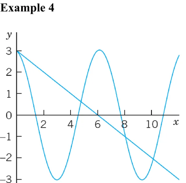
EXAMPLE4 Initial Value Problem Solve the initial value problem

y" + y = 0, y(0) = 3.0, y'(0) = –0.5.

Solution. Step 1. General solution. The functions cos x and sin x are solutions of the ODE (by Exampl e 1), and we take

y = c1 cos x + c2 sin x.

This will turn out to be a general solution as defined below.

continued

Step 2. Particular solution. We need the derivative y' = –c₁ sin x + c₂ cos x. From this and the initial valu es we obtain, since cos 0 = 1 and sin 0 = 0,

y(0) = c₁ = 3.0 and y'(0) = c₂ = –0.5.

This gives as the solution of our initial value problem the particular solution

y = 3.0 cos x – 0.5 sin x.

Figure 28 shows that at x = 0 it has the value 3.0 an d the slope –0.5, so that its tangent intersects the x- axis at x = 3.0/0.5 = 6.0. (The scales on the axes diff

er!) _continued

Fig. 28.

General Solution, Basis, Particular Solution

DEFINITION

A general solution of an ODE (2) on an open interval I is a solution (5) in which y₁ and y₂ are solutions of (2) on I that are not proportional, and c₁ and c₂ are arbitrary constants. These y₁, y₂ are called a basis (or a fundamental system) of solutions of (2) on I.

A particular solution of (2) on I is obtained if we assign specific values to c₁ and c₂ in (5).

Namely, two functions y1 and y2 are called linearly independent on an interval I where they are defined if

(7) k1y1(x) + k2y2(x) = 0 everywhere on I implies

k₁ = 0 and k₂ = 0.

continued

And y1 and y2 are called linearly dependent on I if (7) also holds for some constants k1, k2 not both zer o. Then if k1 ≠ 0 or k2 ≠ 0, we can divide and see that y1 and y2 are proportional,

y₁ = – y₂ or y₂ = – y₁ .

In contrast, in the case of linear independence these functions are not proportional because then we cann ot divide in (7). This gives the following

Basis (Reformulated)

DEFINITION

A basis of solutions of (2) on an open interval I is a pair of linearly independent solutions of (2) on I.

EXAMPLE5 Basis, General Solution, Particular Solution

cos x and sin x in Example 4 form a basis of solution s of the ODE y" + y = 0 for all x because their quotie nt is cot x ≠ const (or tan x ≠ const). Hence y = c1 co s x + c2 sin x is a general solution. The solution y = 3 .0 cos x – 0.5 sin x of the initial value problem is a p articular solution.

EXAMPLE6 Basis, General Solution, Particular Solution

Verify by substitution that y1 = e^x and y2 = e^–x are sol utions of the ODE y" – y = 0. Then solve the initial v alue problem

y – y = 0, y(0) = 6, y'(0) = –2.

continued

Solution. (e^x)" – e^x = 0 and (e^–x)" – e^–x = 0 shows that e^x and e^–x are solutions. They are not proportional, e^x/e^–x = e^2x ≠ const. Hence e^x, e^–x form a basis for all x. We now write down the corresponding general solution and its derivative and equate their values at 0 to the given initial conditions,

y = c1e^x + c2e^–x, y' = c1e^x – c2e^–x,

y(0) = c₁ + c₂ = 6, y'(0) = c₁ – c₂ = –2.

By addition and subtraction, c1 = 2, c2 = 4, so that the answer is y = 2e^x + 4e^–x. This is the particular solution satisfying the two initial conditions.

Find a Basis if One Solution Is Known. Reduction of Order

EXAMPLE7 Reduction of Order if a Solution Is Known.

Basis

Find a basis of solutions of the ODE (x² – x)y" – xy' + y = 0.

Solution. Inspection shows that y1 = x is a solution because y'₁ = 1 and y"₁ = 0, so that the first term van ishes identically and the second and third terms can cel. The idea of the method is to substitute

y = uy₁ = ux, y' = u'x + u, y" = u"x + 2u into the ODE. This gives

(x² – x)(u"x + 2u') – x(u'x + u) + ux = 0.

continued

ux and –xu cancel and we are left with the following ODE, which we divide by x, order, and simplify,

(x² – x)(u"x + 2u') – x²u' = 0, (x² – x)u" + (x – 2)u' = 0.

This ODE is of first order in v = u', namely, (x² – x)v'+

(x – 2)v = 0. Separation of variables and integration gives

continued

We need no constant of integration because we wa nt to obtain a particular solution; similarly in the next integration. Taking exponents and integrating again, we obtain

Since y₁ = x and y₂ = x ln∣x│+ 1 are linearly indepe ndent (their quotient is not constant), we have obtain ed a basis of solutions, valid for all positive x.

2.2 Homogeneous Linear ODEs with Constant Coefficients

We shall now consider second-order homogeneous linear ODEs whose coefficients a and b are constant ,

(1) y" + ay' + by = 0.

These equations have important applications, especi ally in connection with mechanical and electrical vibr ations, as we shall see in Secs. 2.4, 2.8, and 2.9.

continued

How to solve (1)? We remember from Sec. 1.5 that t he solution of the first-order linear ODE with a const ant coefficient k

y' + ky = 0

is an exponential function y = ce^–kx. This gives us th e idea to try as a solution of (1) the function

(2) y = e^λx.

continued

Substituting (2) and its derivatives y = λe^λx and y = λ²e^λx into our equation (1), we obtain (λ² + aλ + b)e^λx = 0.

Hence if λ is a solution of the important characterist ic equation (or auxiliary equation)

(3) λ² + aλ + b = 0

continued

then the exponential function (2) is a solution of the ODE (1). Now from elementary algebra we recall that the roots of this quadratic equation (3) are

(4)

(3) and (4) will be basic because our derivation shows that the functions

(5)

are solutions of (1). Verify this by substituting (5)

into (1). _continued

From algebra we further know that the quadratic equ ation (3) may have three kinds of roots, depending o n the sign of the discriminant a² – 4b, namely,

(Case I) Two real roots if a² – 4b > 0,

(Case II) A real double root if a² – 4b = 0,

(Case III) Complex conjugate roots if a² – 4b < 0.

Case I. Two Distinct Real Roots λ₁ and λ₂

In this case, a basis of solutions of (1) on any interv al is

because y1 and y2 are defined (and real) for all x and their quotient is not constant. The corresponding ge neral solution is

(6)

EXAMPLE1 General Solution in the Case of Distinct Real Roots

We can now solve y" - y = 0 in Example 6 of Sec. 2.

1 systematically. The characteristic equation isλ² – 1

= 0. Its roots areλ₁ = 1 andλ₂ = –1. Hence a basis of solutions is e^x and e^-x and gives the same general so lution as before,

y = c₁e^x + c₂e^-x.

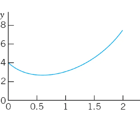
EXAMPLE2 Initial Value Problem in the Case of Distinct Real Roots

Solve the initial value problem

y" + y' – 2y = 0, y(0) = 4, y'(0) = –5.

Solution. Step 1. General solution. The characteri stic equation is

λ² + λ – 2 = 0.

Its roots are

so that we obtain the general solution y = c1e^x + c2e^-2x.

continued

Step 2. Particular solution. Since y'(x) = c1e^x – 2c2

e^-2x, we obtain from the general solution and the initi al conditions

y(0) = c1 + c2 = 4,

y'(0) = c₁ – 2c₂ = –5.

Hence c1 = 1 and c2 = 3. This gives the answer y = e

x + 3e^-2x. Figure 29 shows that the curve begins at y

= 4 with a negative slope (–5, but note that the axes have different scales!), in agreement with the initial c onditions.

continued

Fig. 29.

Case II. Real Double Root λ = – a/2

If the discriminant a² – 4b is zero, we see directly fro m (4) that we get only one root,λ=λ₁ =λ₂ = – a/2, hen ce only one solution,

y1 = e^-(a/2)x.

in the case of a double root of (3) a basis of solution s of (1) on any interval is

e^-ax/2, xe^-ax/2.

The corresponding general solution is (7) y = (c1 + c2x)e^-ax/2.

EXAMPLE3 General Solution in the Case of a Double Root

The characteristic equation of the ODE y" + 6y' + 9y

= 0 isλ² + 6λ+ 9 = (λ+ 3)² = 0. It has the double root λ = –3. Hence a basis is e^-3x and xe^-3x. The correspo nding general solution is y = (c1 + c2x)e^-3x.

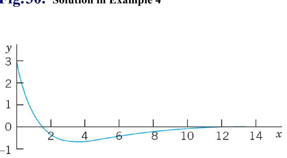
EXAMPLE4 Initial Value Problem in the Case of a Double Root

Solve the initial value problem

y" + y' + 0.25y = 0, y(0) = 3.0, y'(0) = –3.5.

Solution. The characteristic equation is λ² +λ+ 0.25

= (λ+ 0.5)² = 0. It has the double rootλ= –0.5. This gi ves the general solution

y = (c1 + c2x)e^-0.5x.

continued

We need its derivative

y' = c2e^-0.5x – 0.5(c1 + c2x)e^-0.5x.

From this and the initial conditions we obtain y(0) = c₁ = 3.0, y'(0) = c₂ – 0.5c₁ = 3.5;

hence c2 = –2.

The particular solution of the initial value problem is y = (3 – 2x)e^-0.5x. See Fig. 30.

continued

Fig. 30.

Case III. Complex Roots – 1/2a + iω and – 1/2a – iω

This case occurs if the discriminant a² – 4b of the ch aracteristic equation (3) is negative. In this case, the roots of (3) and thus the solutions of the ODE (1) co me at first out complex. However, we show that from them we can obtain a basis of real solutions

(8) y₁ = e^-ax/2 cos ωx, y₂ = e^-ax/2 sin ωx

(ω > 0)

continued

where ω² = b – 1/4a². It can be verified by substitutio n that these are solutions in the present case. We s hall derive them systematically after the two exampl es by using the complex exponential function. They f orm a basis on any interval since their quotient cot x is not constant. Hence a real general solution in Cas e III is

(9) y = e^-ax/2 (A cos ωx + B sin ωx)

(A, B arbitrary).

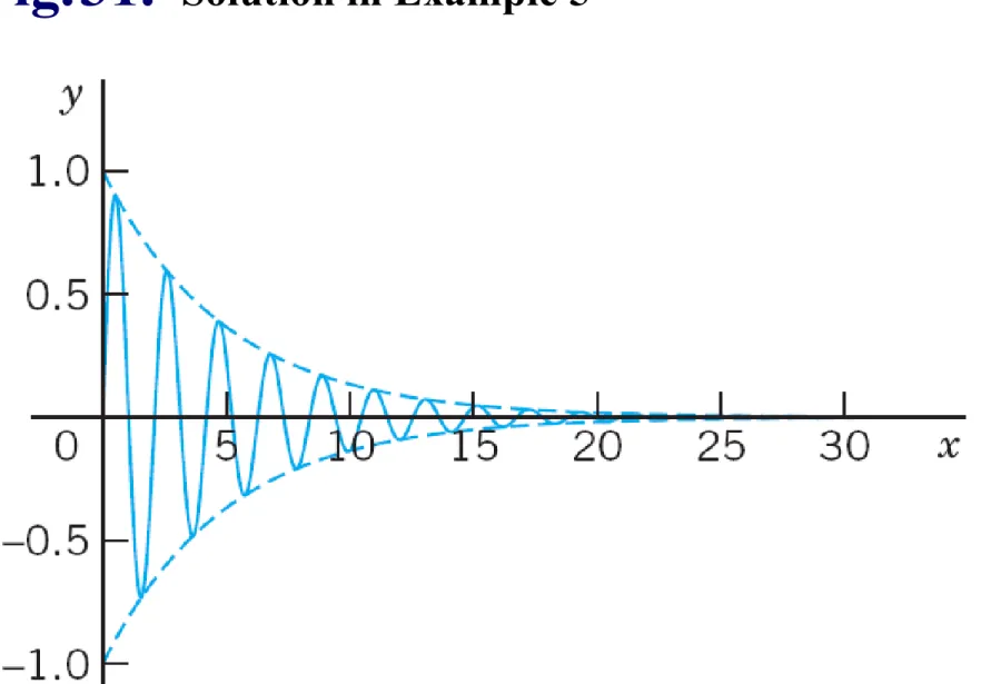
EXAMPLE5 Complex Roots. Initial Value Problem Solve the initial value problem

y" + 0.4y' + 9.04y = 0, y(0) = 0, y'(0) = 3.

Solution. Step1. General solution. The characteristic equation is λ² + 0.4λ+ 9.04 = 0. It has the roots –0.2 ± 3i. Hence ω = 3, and a general solution (9) is

y = e^-0.2x(A cos 3x + B sin 3x).

Step 2. Particular solution. The first initial condition gives y(0) = A = 0. The remaining expression is y = B e^-0.2x sin 3x. We need the derivative (chain rule!)

continued

y' = B(–0.2e^-0.2x sin 3x + 3e^-0.2x cos 3x).

From this and the second initial condition we obtain y'(0) = 3B = 3. Hence B = 1. Our solution is

y = e^-0.2x sin 3x.

Figure 31 shows y and the curves of e^-0.2x and –e^-0.2x (dashed), between which the curve of y oscillates. S uch “damped vibrations” (with x = t being time) have important mechanical and electrical applications, as we shall soon see (in Sec. 2.4).

continued

Fig. 31.

EXAMPLE6 Complex Roots A general solution of the ODE

y" + ω²y = 0 (ω constant, not zero) is

y = A cos ωx + B sin ωx.

With ω = 1 this confirms Example 4 in Sec. 2.1.

Summary of Cases I–III

Derivation in Case III.

Complex Exponential Function

If verification of the solutions in (8) satisfies you, skip the systematic derivation of these real solutions fro m the complex solutions by means of the complex e xponential function e^z of a complex variable z = r + it . We write r + it, not x + iy because x and y occur in t he ODE. The definition of e^z in terms of the real func tions e^r, cos t, and sin t is

(10) e^z = e^{r + it} = e^re^it = e^r(cos t + i sin t).

continued

(11) e^it = cos t + i sin t,

called the Euler formula. Multiplication by e^r gives (10).

For later use we note that e^-it = cos (–t) + i sin (–t) c os t – i sin t, so that by addition and subtraction of thi s and (11),

(12)

2.3 Differential Operators. Optional

EXAMPLE1 Factorization, Solution of an ODE Factor P(D) = D² – 3D – 40I and solve P(D)y = 0.

Solution. D² – 3D – 40I = (D – 8I)(D + 5I) because I²

= I. Now (D – 8I)y = y – 8y = 0 has the solution y₁ = e^8x. Similarly, the solution of (D + 5I)y = 0 is y₂ = e^-5x. This is a basis of P(D)y = 0 on any interval. From th e factorization we obtain the ODE, as expected,

continued

(D – 8I)(D + 5I)y = (D – 8I)(y' + 5y)

= D(y' + 5y) – 8(y' + 5y) = y'' + 5y' – 8y' – 40y = y'' – 3y' – 40y = 0.

Verify that this agrees with the result of our method i n Sec. 2.2. This is not unexpected because we facto red P(D) in the same way as the characteristic polyn omial P(λ) = λ² – 3λ – 40.

2.4 Modeling: Free Oscillations (Mass–Spring System)

Linear ODEs with constant coefficients have importa nt applications in mechanics, as we show now (and i n Sec. 2.8), and in electric circuits (to be shown in S ec. 2.9). In this section we consider a basic mechani cal system, a mass on an elastic spring (“mass-sprin g system,” Fig. 32), which moves up and down. Its model will be a homogeneous linear ODE.

Setting Up the Model

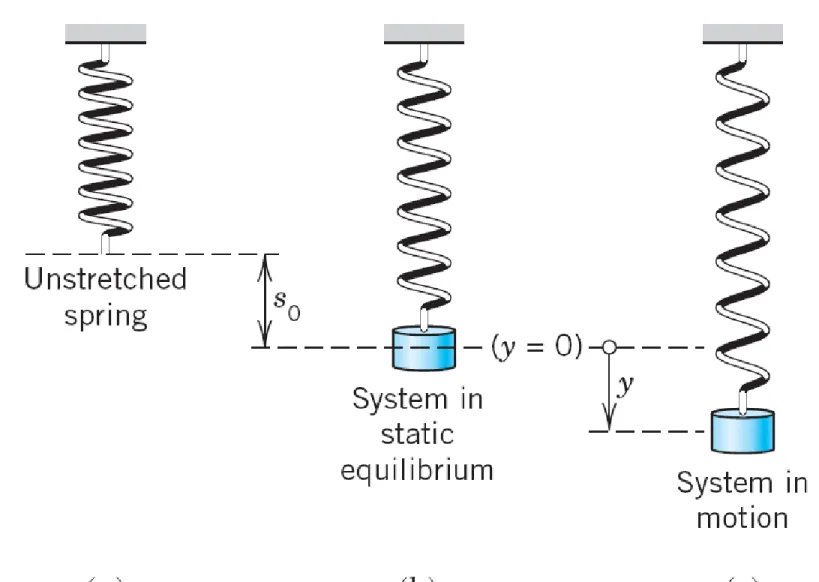
We take an ordinary spring that resists compression as well extension and suspend it vertically from a fixed support, as shown in Fig. 32. At the lower end of the spring we attach a body of mass m. We assume m to be so large that we can neglect the mass of the spring. If we pull the body down a certain distance and then release it, it starts moving.

We assume that it moves strictly vertically.

continued

Fig. 32.

continued

How can we obtain the motion of the body, say, the displacement y(t) as function of time t? Now this moti on is determined by Newton’s second law

(1) Mass × Acceleration = my" = Force

where y" = d²y/dt² and “Force” is the resultant of all t he forces acting on the body.

(For systems of units and conversion factors, see th e inside of the front cover.)

We choose the downward direction as the positiv e direction, thus regarding downward forces as posi tive and upward forces as negative.

continued

Consider Fig. 32. The spring is first unstretched. We now attach the body. This stretches the spring by an amount s₀ shown in the figure. It causes an upward f orce F₀ in the spring. Experiments show that F₀ is pr oportional to the stretch s0, say,

(2) F₀ = –ks₀ (Hooke’s law2).

k (> 0) is called the spring constant (or spring mod ulus). The minus sign indicates that F₀ points upwar d, in our negative direction. Stiff springs have large k . (Explain!)

continued

The extension s0 is such that F0 in the spring balanc es the weight W = mg of the body (where g = 980 c m/sec² = 32.17 ft /sec² is the gravitational constant).

Hence F₀ + W = –ks₀ + mg = 0. These forces will not affect the motion. Spring and body are again at rest.

This is called the static equilibrium of the system (Fig. 32b). We measure the displacement y(t) of the body from this ‘equilibrium point’ as the origin y = 0, downward positive and upward negative.

continued

From the position y = 0 we pull the body downward.

This further stretches the spring by some amount y

> 0 (the distance we pull it down). By Hooke’s law th is causes an (additional) upward force F₁ in the sprin g,

F₁ = –ky.

F1 is a restoring force. It has the tendency to restor e the system, that is, to pull the body back to y = 0.

Undamped System: ODE and Solution

Every system has damping—otherwise it would keep moving forever. But practically, the effect of damping may often be negligible, for example, for the motion of an iron ball on a spring during a few minutes. The n F₁ is the only force in (1) causing the motion. Henc e (1) gives the model my" = –ky or

(3) my" + ky = 0.

We obtain as a general solution (4) y(t) = A cos ω₀ t B sin ω₀ t,

The corresponding motion is called a harmonic osc illation.

continued

Since the trigonometric functions in (4) have the peri od 2π/ω₀, the body executes ω₀/2π cycles per seco nd. This is the frequency of the oscillation, which is also called the natural frequency of the system. It i s measured in cycles per second. Another name for cycles/sec is hertz (Hz).

The sum in (4) can be combined into a phase-shifted cosine with amplitude and phase angle δ

= arctan (B/A),

(4*) y(t) = C cos (ω₀t – δ).

continued

Fig. 33.

EXAMPLE1 Undamped Motion. Harmonic Oscillation If an iron ball of weight W = 98 nt (about 22 lb) stretc hes a spring 1.09 m (about 43 in.), how many cycles per minute will this mass–spring system execute? W hat will its motion be if we pull down the weight an a dditional 16 cm (about 6 in.) and let it start with zero initial velocity?

Solution. Hooke’s law (2) with W as the force and 1.

09 meter as the stretch gives W = 1.09k; thus k = W/

1.09 = 98/1.09 = 90 [kg/sec²] = 90 [nt/meter]. The m ass is m = W/g = 98/9.8 = 10 [kg]. This gives the fre quency ω0/(2π) = (k/m)^1/2/(2π) = 3/(2π) = 0.48 [Hz] = 29 [cycles/min].

continued

From (4) and the initial conditions, y(0) = A = 0.16 [meter] and y'(0) = ω₀B = 0. Hence the motion is

y(t) = 0.16 cos 3t [meter] or 0.52 cos 3t [ft]

If you have a chance of experimenting with a mass–

spring system, don’t miss it. You will be surprised ab out the good agreement between theory and experi ment, usually within a fraction of one percent if you measure carefully.

continued

Fig. 34.

Damped System: ODE and Solutions

We now add a damping force F2 = –cy'

to our model my" = –ky, so that we have my" = –ky – cy' or

(5) my" + cy' + ky = 0.

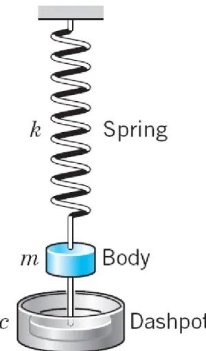
Physically this can be done by connecting the body t o a dashpot; see Fig. 35. We assume this new force to be proportional to the velocity y' = dy/dt, as shown . This is generally a good approximation, at least for small velocities.

continued

Fig. 35.

continued

c is called the damping constant. We show that c i s positive. If at some instant, y' is positive, the body i s moving downward (which is the positive direction).

Hence the damping force F₂ = –cy', always acting ag ainst the direction of motion, must be an upward forc e, which means that it must be negative, F₂ = –cy' <

0, so that – c < 0 and c > 0. For an upward motion, y' < 0 and we have a downward F₂ = –cy' > 0; hence –c < 0 and c > 0, as before.

continued

The ODE (5) is homogeneous linear and has constant coefficients. Hence we can solve it by the method in Sec. 2.2. The characteristic equation is (divide (5) by m)

By the usual formula for the roots of a quadratic equation we obtain, as in Sec. 2.2,

(6)

continued

It is now most interesting that depending on the amount of damping (much, medium, or little) there will be three types of motion corresponding to the three Cases I, II, II in Sec. 2.2:

Discussion of the Three Cases

Case I. Overdamping

If the damping constant c is so large that c² > 4mk, t hen λ1 and λ2 are distinct real roots. In this case the corresponding general solution of (5) is

(7) y(t) = c₁e^-(α-β)t + c₂e^-(α+β)t.

continued

We see that in this case, damping takes out energy so quickly that the body does not oscillate. For t > 0 both exponents in (7) are negative because α > 0, β

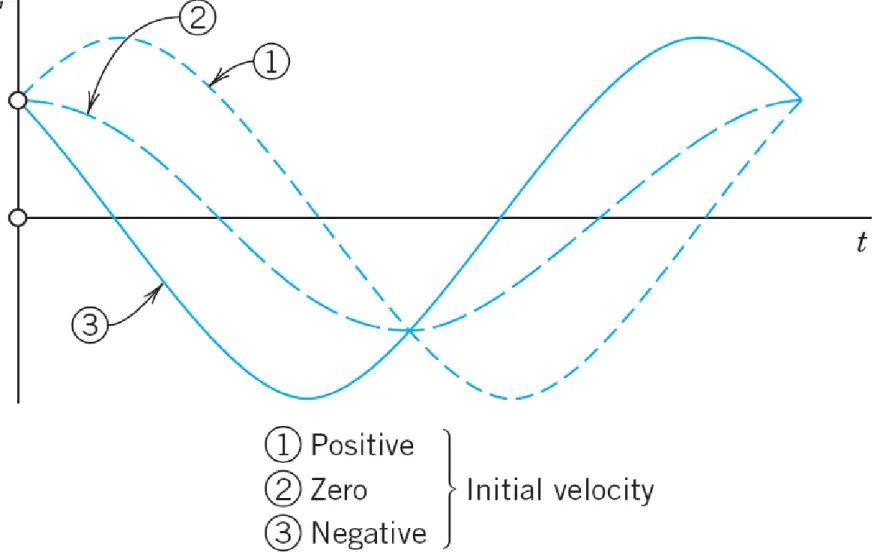
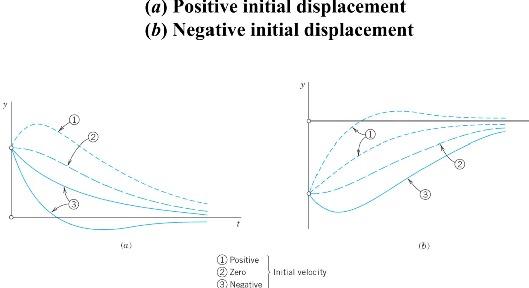
> 0, and β² = α² – k/m < α2. Hence both terms in (7) approach zero as t → ∞. Practically speaking, after a sufficiently long time the mass will be at rest at the static equilibrium position (y = 0). Figure 36 shows (7) for some typical initial conditions.

continued

Fig. 36.

(b) Negative initial displacement

Case II. Critical Damping

Critical damping is the border case between nonosci llatory motions (Case I) and oscillations (Case III). It occurs if the characteristic equation has a double ro ot, that is, if c² = 4mk, so that β = 0, λ₁ = λ₂ = –α. The n the corresponding general solution of (5) is

(8) y(t) = (c1 + c2t)e^-αt.

continued

This solution can pass through the equilibrium positi on y = 0 at most once because e^-αt is never zero and c₁ + c₂t can have at most one positive zero. If both c₁ and c₂ are positive (or both negative), it has no positi ve zero, so that y does not pass through 0 at all. Fig ure 37 shows typical forms of (8). Note that they loo k almost like those in the previous figure.

continued

Fig. 37.

Case III. Underdamping

This is the most interesting case. It occurs if the da mping constant c is so small that c² < 4mk. Then in (6) is no longer real but pure imaginary, say,

(9) β = iω*

(We write ω* to reserve for driving and electromotiv e forces in Secs. 2.8 and 2.9.) The roots of the char acteristic equation are now complex conjugate,

λ1 = –α+ iω*, λ2 = –α– iω*

continued

with α = c/(2m), as given in (6). Hence the correspo nding general solution is

(10) y(t) = e^-αt(A cos ω*t + B sin ω*t) = Ce^-αt cos (ω*t – δ)

where C² = A² + B² and tan δ = B/A, as in (4*).

This represents damped oscillations. Their curve li es between the dashed curves y = Ce^-αt and y = –C e^-αt in Fig. 38, touching them when ω*t –δ is an integ er multiple of π because these are the points at whic h cos (ω*t –δ) equals 1 or –1.

continued

The frequency is ω*/(2π) Hz (hertz, cycles/sec). Fro m (9) we see that the smaller c (> 0) is, the larger is ω* and the more rapid the oscillations become. If c a pproaches 0, then ω* approaches ω₀ = (k/m)^1/2, givin g the harmonic oscillation (4), whose frequency ω₀/ (2π) is the natural frequency of the system.

continued

Fig. 38.

EXAMPLE2 The Three Cases of Damped Motion

How does the motion in Example 1 change if we change the damping constant c to one of the following three values, with y(0) = 0.16 and y'(0) = 0 as before?

(I) c = 100 kg/sec, (II) c = 60 kg/sec, (III) c = 10 kg/sec.

Solution. It is interesting to see how the behavior of the system changes due to the effect of the damping, which takes energy from the system, so that the oscillations decrease in amplitude (Case III) or even disappear (Cases II and I).

continued

(I) With m = 10 and k = 90, as in Example 1, the mo del is the initial value problem

10y" +100y' + 90y = 0, y(0) = 0.16 [meter], y'(0) = 0 .

The characteristic equation is 10λ² + 100λ+ 90 = 10(λ+ 9)(λ+ 1) = 0. It has the roots –9 and –1. This g ives the general solution

y = c1e^-9t + c2e^-t.

We also need y' = –9c₁e^-9t – c₂e^-t.

continued

The initial conditions give c1 + c2 = 0.16, –9c1 – c2 = 0. The solution is c1 = –0.02, c2 = 0.18. Hence in the overdamped case the solution is

y = –0.02e^-9t + 0.18e^-t.

It approaches 0 as t → ∞. The approach is rapid; aft er a few seconds the solution is practically 0, that is, the iron ball is at rest.

continued

(II) The model is as before, with c = 60 instead of 100. T he characteristic equation now has the form 10λ² + 60λ+

90 = 10(λ+ 3)² = 0. It has the double root –3. Hence the c orresponding general solution is

y = (c₁ + c₂t)e^-3t.

We also need y' = (c₂ – 3c₁ – 3c₂t)e^-3t.

The initial conditions give y(0) = c₁ = 0.16, y'(0) = c₂ – 3c₁

= 0, c2 = 0.48. Hence in the critical case the solution is y = (0.16 + 0.48t)e^-3t.

It is always positive and decreases to 0 in a monotone fa shion.

continued

(III) The model now is 10y" + 10y' + 90y = 0. Since c

= 10 is smaller than the critical c, we shall get oscilla tions. The characteristic equation is 10λ² + 10λ+ 90

= . It has the complex roots [se e (4) in Sec. 2.2 with a = 1 and b = 9]

This gives the general solution

y e^-0.5t(A cos 2.96t + B sin 2.96t).

Thus y(0) = A = 0.16. We also need the derivative

continued

y = e^-0.5t(–0.5A cos 2.96t – 0.5B sin 2.96t – 2.96A sin 2.96t + 2.96B cos 2.96t).

Hence y'(0) = –0.5A + 2.96B = 0, B = 0.5A/2.96 = 0.027.

This gives the solution

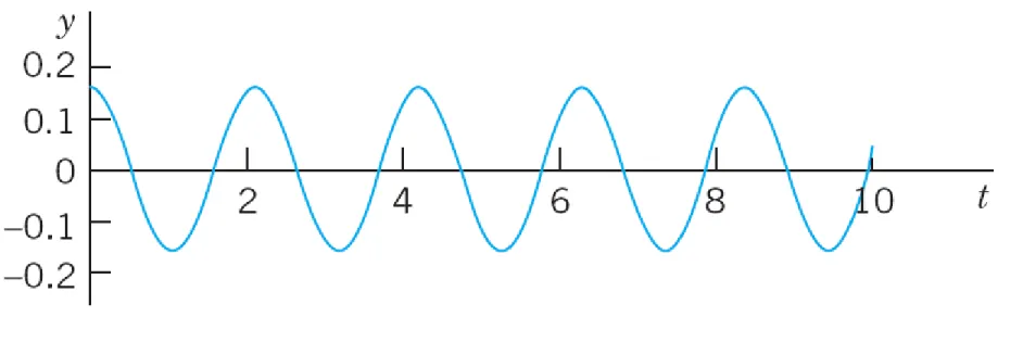
y = e^-0.5t(0.16 cos 2.96t + 0.027 sin 2.96t) = 0.162e^-0.5t cos (2.96t – 0.17).

We see that these damped oscillations have a smaller frequency than the harmonic oscillations in Example 1 by about 1% (since 2.96 is smaller than 3.00 by about 1%). Their amplitude goes to zero. See Fig. 39.

continued

Fig. 39.

2.5 Euler–Cauchy Equations

Euler–Cauchy equations are ODEs of the form (1) x²y" + axy' + by = 0

with given constants a and b and unknown y(x). We substitute

(2) y = x^m

and its derivatives y' = mx^m-1 and y'' = m(m – 1)x^m-2 i nto (1).

This gives

x²m(m – 1)x^m-2 + axmx^m-1 + bx^m = 0.

continued

We now see that (2) was a rather natural choice bec ause we have obtained a common factor x^m. Droppi ng it, we have the auxiliary equation m(m – 1) + am + b = 0 or

(3) m² + (a – 1)m + b = 0. (Note: a – 1, not a.) Hence y = x^m is a solution of (1) if and only if m is a r

oot of (3).

Case I. If the roots m1 and m2 are real and different, then solutions are

and

They are linearly independent since their quotient is not constant. Hence they constitute a basis of solutions of (1) for all x for which they are real. The corresponding general solution for all these x is

(5) (c1, c2

arbitrary).

EXAMPLE1 General Solution in the Case of Different Real Roots

The Euler–Cauchy equation

x²y" + 1.5xy' – 0.5y = 0 has the auxiliary equation

m² + 0.5m – 0.5 = 0. (Note: 0.5, not 1.5!) The roots are 0.5 and –1. Hence a basis of solutions

for all positive x is y1 = x^0.5 and y2 = 1/x and gives the general solution

(x > 0).

Case II. Equation (4) shows that the auxiliary equati on (3) has a double root m1 = 1/2(1 – a) if and only i f (1 – a)² – 4b = 0. The Euler–Cauchy equation (1) th en has the form

(6)

In this “critical case,” a basis of solutions for positive x is y1 = x^m and y2 = x^m ln x, where m = 1/2(1 – a). Li near independence follows from the fact that the qu otient of these solutions is not constant. Hence, for a ll x for which y₁ and y₂ are defined and real, a gener al solution is

(7) m = 1/2(1 – a)

EXAMPLE2 General Solution in the Case of a Double Root

The Euler–Cauchy equation x²y" – 5xy' + 9y = 0 has the auxiliary equation m² – 6m + 9 = 0. It has the do uble root m = 3, so that a general solution for all posi tive x is

y = (c1 + c2 ln x) x³.

Case III. The case of complex roots is of minor pract ical importance, and it suffices to present an exampl e that explains the derivation of real solutions from c omplex ones.

EXAMPLE3 Real General Solution in the Case of Complex Roots

The Euler–Cauchy equation

x²y" + 0.6xy' + 16.04y = 0

has the auxiliary equation m² – 0.4m + 16.04 = 0. Th e roots are complex conjugate, m1 = 0.2 + 4i and m2

= 0.2 – 4i, where i = (–1)^1/2. (We know from algebra t hat if a polynomial with real coefficients has complex roots, these are always conjugate.) Now use the tric k of writing x = e^{ln x} and obtain

continued

Next apply Euler’s formula (11) in Sec. 2.2 with t = 4 ln x to these two formulas. This gives

Add these two formulas, so that the sine drops out, and divide the result by 2. Then subtract the second formula from the first, so that the cosine drops out, a nd divide the result by 2i. This yields

x^0.2 cos (4 ln x) and x^0.2 sin (4 ln x)

continued

respectively. By the superposition principle in Sec. 2 .2 these are solutions of the Euler–Cauchy equation (1). Since their quotient cot (4 ln x) is not constant, t hey are linearly independent. Hence they form a bas is of solutions, and the corresponding real general s olution for all positive x is

(8) y = x^0.2[A cos (4 ln x) + B sin (4 ln x)].

Figure 47 shows typical solution curves in the three cases discussed, in particular the basis functions in Examples 1 and 3.

continued

Fig. 47.

EXAMPLE4 Boundary Value Problem.

Electric Potential Field Between Two Concentric Spheres

Find the electrostatic potential v = v(r) between two concentric spheres of radii r1 = 5 cm and r2 = 10 cm kept at potentials v1 = 110 V and v2 = 0, respectively.

Physical Information. v(r) is a solution of the Euler –Cauchy equation rv" + 2v' = 0, where v' = dv/dr.

continued