大離差理論在系統風險和投資組合最佳化的應用

國立臺灣大學理學院應用數學科學研究所 碩士論文

Institute of Applied Mathematical Sciences College of Science

National Taiwan University Master Thesis

大離差理論在系統風險和投資組合最佳化的應用

Applications of Large Deviation Theory to Systemic Risk and Portfolio Optimization

郭宣宏 Hsuan-Hung Kuo

指導教授：韓傳祥博士

Advisor: Chuan-Hsiang Han, Ph.D.

中華民國 108 年 6 月

June 2019

iii

摘要

這份論文有兩部分。在第一部分，我們會用重要抽樣法來估計稀 有事件的期望值。在常態分配或是布朗運動模型下，可以證明我們提 出的方法是有效率的。我們也會說明如何應用重要抽樣法來評估系統 風險。在第二部分，我們會應用大離差理論在有限時間的投資最佳化 上面。

關鍵詞：重要抽樣法、漸進最佳、大離差、體系風險、投資組合最佳 化

v

Abstract

There are two parts in this paper. In the first part, we will focus on estimating the expectations under a rare event with the importance sampling method. Under Normal distribution or Brownian motion, we can prove that our proposed method is efficient. We will also show how to apply the importance sampling method to measure the systemic risk. In the second part, we will apply large deviation theory to the finite-horizon investment optimization.

Keywords: importance sampling, asymptotic optimality, large deviation, systemic risk, optimal portfolio

Contents

摘要 iii

Abstract v

1 Introduction 1

Part 1 3

2 Standard Normal Case 4

2.1 Change measure . . . 4 2.2 Asymptotic variance analysis . . . 5 2.3 Numerical results . . . 7

3 Brownian Motion Case 8

3.1 Change measure . . . 8 3.2 Asymptotic variance analysis . . . 9 3.3 Numerical results . . . 11

4 Geometric Brownian Motion Case 12

4.1 Change measure . . . 12 4.2 Asymptotic variance analysis . . . 13 4.3 Numerical results . . . 17

5 Applications to Measuring Systemic Risk 18

5.1 Stochastic Volatility model . . . 18 5.2 First Passage Time Case . . . 20

Part 2 23

6 Optimal Finite-Horizon Investment 24

6.1 Constant Investment Strategy . . . 25 6.2 Deterministic Investment Strategy . . . 28

7 Conclusion 31

References 32

List of Tables

2.1 Standard normal case . . . 7 3.1 Brownian motion case . . . 11 4.1 Geometric Brownian motion case . . . 17 5.1 Results of basic Monte Carlo simulation and importance sampling scheme

with N = 160000, T = 0.5, dt = 0.002, µ_m = 0.1, µ_i = 0.08, κ_m = 5, κi = 3, ξm = 2, ξi = 1, θm = 0.5, θi = 0.3, αi = 5, βi = 1, m = 0.5, ρ_i = 0.5, ρ_m = 0.5. . . . 20 5.2 Results of basic Monte Carlo simulation and importance sampling scheme

with N = 40000, T = 0.5, dt = 0.002, µ_i = 0.08, µ_m = 0.1, σ_i = 0.3, σ_m = 0.5, ρ = 0.7. . . . 22

Chapter 1

Introduction

It is a trend to use Monte Carlo simulation to estimate credit risk. However, it is not effi- cient when the event become rare. For example, let Z be a random variable that follows the standard normal distribution. We are interested in the expectation E[Z1(Z < c)], where c is a negative constant. It is easy to compute the closed form−^√1_2πe^−c22 . However, when c is very small, we can see that the value will become very small, which makes it inefficient to use crude Monte Carlo to estimate it. That is, we need to sample a lot of times so that we can have a small standard error.

The importance sampling method helps us to solve the ”inefficient” problem. More specif- ically, the importance sampling method helps to reduce the variance [9]. The idea of im- portance sampling is to find a suitable change of measure so that the rare events we are interested in will become ”not rare” under the new measure, which will be called ˜P in this paper. Also, we need to reduce the variance of estimation under this new measure ˜P . Since

V arP˜ = EP˜[(f (Z)dP

d ˜P)²]− (EP^˜[f (Z)dP d ˜P])²

= EP˜[(f (Z)dP

d ˜P)²]− (E[f(Z)])²,

we can see that the variance equals to 0 if we could minimize the second moment under the measure ˜P . However, it is difficult to minimize it directly since the minimization often relates to solving a nonlinear equation. Thus, we seek another way called ”asymp- totically optimal” property to solve it [9]. That is, we will check if lim_{c→−∞ c}¹2 ln M₂ =

2 limc→−∞ 1

c² ln M1under the measure ˜P , where M1, M2are the first moment and the sec- ond moment, respectively. If it does, it implies that the importance sampling we proposed is ”efficient”.

On the other hand, a lot of researchers use Importance Sampling to apply the theory of large deviation to analyze the asymptotic properties of the tail probability. The famous theories are Cramer Theorem, Schilder’s Theorem, Freidlin-Wentzell Theorem, etc. In financial applications, some researchers let the time T go to infinity so that these large de- viation theories can be easily applied. [8] provides a large deviations approach to optimal long-term investment. However, some investors would like to earn their money as soon as possible. Thus, we will try to apply the theory of large deviations to the finite-horizon investment.

This paper is composed of two parts. In the first part, we will apply Importance Sampling to estimate the expectation of a random variable under a rare event. In Chapter 2, we are going to apply the method under the standard normal distribution. In Chapter 3 and 4, we will extend it to Brownian motion and geometric Brownian motion. In Chapter 5, we present some applications to estimate systemic risk under different models. In the second part, we will apply the theory of large deviation to the finite-horizon investment, which will be represented in Chapter 6.

Part 1

Large Deviation Theory applied to Systemic Risk

In this part, we will use importance sampling method to measure the systemic risk under different models. In order to do this, we need to estimate the form E[1(X < c)] and E[X1(X < c)], where X is a random variable and c is a (usually negative) constant.

There have been some papers about how to estimate E[1(X < c)] efficiently, such as [1]

and [2]. Thus, we will focus on E[X1(X < c)] in this part.

Chapter 2

Standard Normal Case

Suppose Xi = ρXM +√

1− ρ²Y , where XM, Y are independent standard normal distri- bution, and ρ is correlation between X_iand X_M. We are going to estimate E[X_i1(X_M <

c)]. When the value c is very small, it is difficult to use Monte Carlo to estimate. Thus, we will use importance sampling by choosing a new measure ˜P such that the event{XM < c} is no more ”rare” under this measure.

2.1 Change measure

Note that

E[X_i1(X_M < c)] = E[(ρX_M +√

1− ρ²Y )1(X_M < c)]

= ρE[X_M1(X_M < c)] +√

1− ρ²E[Y 1(X_M < c)]

We can see that the second term is equal to 0 since X_M and Y are independent. Thus, we just need to consider the first term.

The easiest way to choose a new measure ˜P such that the event {XM < c} is no more

”rare” under this measure is to make the mean of XM be c. That means XM will be a normal distribution with the mean c and the variance 1 under the new measure ˜P . Then

we can derive that

dP d ˜P =

√1

2πe^−X22M

√1

2πe^{−(XM −c)}

2 2

= e^−cXM+c22 . Due to the above, we can rewrite the first term as:

E[XM1(XM < c)] = ˜E[XMexp(−cXM + c²

2)1(XM < c)].

2.2 Asymptotic variance analysis

The first moment is

M₁ =−ρE[XM1(X_M < c)]

=−ρ

∫ c

−∞

√z

2πe^−z22 dz

= ρ

√2πe^−c22 .

It implies that

c→−∞lim 1

c² ln M₁ =−1 2.

Suppose X_M ∼ N(−c, 1), Z ∼ N(0, 1) under ˆP . Then the second moment is M₂ = ˜E[X_i²exp(−2cXM + c²)1(X_M < c)]

= e^c2E[Xˆ _i²exp(−2cXM)1(XM < c)d ˜P d ˆP]

= e^c2E[Xˆ _i²exp(−2cXM)1(XM < c)e^2cXM]

= e^c2E[Xˆ _i²1(X_M < c)]

= ρ²e^c2E[Xˆ _M² 1(X_M < c)] + (1− ρ²)e^c2E[Yˆ ²1(X_M < c)]

= ρ²e^c2E[(Zˆ − c)²1(Z < 2c)] + (1− ρ²)e^c2E[1(Z < 2c)]ˆ

= ρ²e^c2{ ˆE[Z²1(Z < 2c)]− 2c ˆE[Z1(Z < 2c)] + c²E[1(Z < 2c)]ˆ } + (1− ρ²)e^c2Φ(2c)

= ρ²e^c2{

∫ _2c

−∞

z²

√2πe^−z22 dz− 2c

∫ _2c

−∞

√z

2πe^−z22 dz + c²Φ(2c)} + (1− ρ²)e^c2Φ(2c)

= ρ²e^c2(1 + c²)Φ(2c) + (1− ρ²)e^c2Φ(2c)

= (ρ²c²+ 1)e^c2Φ(2c),

where Φ(z) is the cdf of a standard normal.

There is an important approximation to Φ(z):

z→−∞lim Φ(z) = 1

√2π(−z)e^−z22 .

It implies that

c→−∞lim 1 c² ln M2

= lim

c→−∞

1

c²[c²+ ln(ρ²c²+ 1) + ln( 1

√2π(−2c))− 2c²]

=−1.

Thus, we have the following theorem.

Theorem 1. Suppose Xi = ρXM +√

1− ρ²Y , where XM, Y are independent standard

M₂ = ˜E[X_i²1(X_M < c)(dP d ˜P)²].

Then,

c→−∞lim 1

c² ln M2 = 2 lim

c→−∞

1

c² ln M1.

2.3 Numerical results

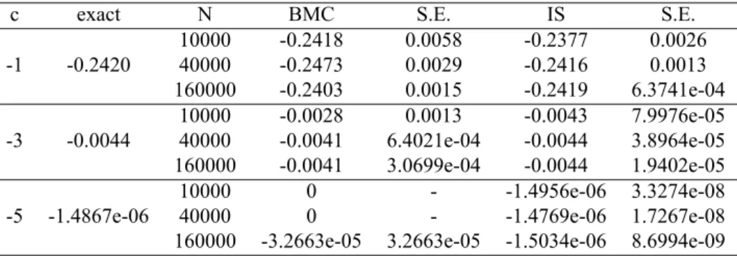
The numerical results are shown below. N is the simulation number. The value simulated by basic Monte Carlo (BMC), importance sampling (IS) and the corresponding standard error (S.E.) are given in the table. We also compare the value with the exact answer (exact).

Table 2.1: Standard normal case

c exact N BMC S.E. IS S.E.

10000 -0.2418 0.0058 -0.2377 0.0026

-1 -0.2420 40000 -0.2473 0.0029 -0.2416 0.0013

160000 -0.2403 0.0015 -0.2419 6.3741e-04 10000 -0.0028 0.0013 -0.0043 7.9976e-05 -3 -0.0044 40000 -0.0041 6.4021e-04 -0.0044 3.8964e-05 160000 -0.0041 3.0699e-04 -0.0044 1.9402e-05

10000 0 - -1.4956e-06 3.3274e-08

-5 -1.4867e-06 40000 0 - -1.4769e-06 1.7267e-08

160000 -3.2663e-05 3.2663e-05 -1.5034e-06 8.6994e-09

We can see that the basic Monte Carlo method can hardly sample a rare event when c =

−5, while the importance sampling method we provide gives an accurate estimation. In addition, the sample error of importance sampling scheme is smaller than that of basic Monte Carlo method.

Chapter 3

Brownian Motion Case

Let W_{M t}, Z_tbe independent Brownian motion. Define Wit = ρWM t+√

1− ρ²Zt,

where ρ is a correlation between W_itand W_{M t}. Then W_it is also a Brownian motion. In this chapter, we are going to estimate E[W_iT1(W_{M T} < c)].

3.1 Change measure

Note that if c becomes very small, the probability of the event {WM T < c} will also be small, which means that it will be inefficient to use crude Monte Carlo method. Thus, we need to find a new measure ˜P such that the event{WM T < c} would be no more ”rare”

under this measure. The following theorem helps us to find a good measure.

Girsanov’s Theorem. [6] Let W_t, 0≤ t ≤ T be a Brownian motion. Let Θt, 0≤ t ≤ T be an adapted process. Define

Z_t= exp{

∫ t 0

Θ_uW_u− 1 2

∫ t 0

Θ²_udu}, W˜ = W −

∫ t

Θ du,

We also define a new probability measure ˜P by the formula P˜_A=

∫

A

Z_ωdP_ωfor all A∈ F.

Set Z = Z_T. Then E[Z] = 1 and under the probability measure ˜P , the process ˜W_t, 0≤ t ≤ T , is also a Brownian motion.

By the Girsanov’s Theorem, we can define dP

d ˜P = e^{−αWM T+12α2T}, W˜_{M T} = W_{M T} − αT,

where α is a constant and ˜W_{M T} is a Brownian motion under ˜P .

Next, we are going to determine the constant α. If we hope to make the event{WM T < c} no more ”rare”, we can simply let ˜E[WM T] = c. That is to say,

E[W˜ _{M T}] = ˜E[ ˜W_{M T} + αT ] = αT = c, which means that α = _T^c.

3.2 Asymptotic variance analysis

Note that W_{M T} ∼ N(0, T ) since WM T is a Brownian motion. So we can get the first moment as following:

M₁ =−E[WiT1(W_{M T} < c)]

=−ρE[WM T1(W_{M T} < c)]

=−ρ

∫ c

−∞

√x

2πTe^−x22Tdx

= ρ√

√ T

2πe^−2Tc2. It implies that

c→−∞lim 1

c² ln M₁ =− 1 2T.

Before we consider the second moment, we define a new measure ˆP by dP

d ˆP = e^{αWM T+12α2T} Wˆ_{M T} = W_{M T} + αT,

where ˆW_{M T} is a Brownian motion under ˆP . Then we can calculate the second moment as follows:

M₂ = ˜E[W_iT² 1(W_{M T} < c)(dP d ˜P)²]

= E[W_iT² 1(W_{M T} < c)dP d ˜P]

= ˆE[W_iT² 1(W_{M T} < c)dP d ˜P

dP d ˆP]

= ˆE[W_iT² 1(WM T < c)e^α2T]

= e^α2TE[(ρWˆ _{M T} +√

1− ρ²Z_T)²1(W_{M T} < c)]

= e^α2T{ ˆE[ρ²W_{M T}² 1(W_{M T} < c)] + ˆE[(1− ρ²)Z_T²1(W_{M T} < c)]}

= ρ²e^α2TE[Wˆ _{M T}² 1(WM T < c)] + (1− ρ²)e^α2TT ˆE[1(WM T < c)]

= ρ²e^α2TE[( ˆˆ W_{M T} − αT )²1( ˆW_{M T} < 2c)] + (1− ρ²)e^α2TT Φ( 2c

√T)

= ρ²e^α2T{ ˆE[ ˆW_{M T}² 1( ˆW_{M T} < 2c)]− 2αT ˆE[ ˆW_{M T}1( ˆW_{M T} < 2c)]

+ α²T²E[1( ˆˆ W_{M T} < 2c)]} + (1 − ρ²)e^α2TT Φ( 2c

√T)

= ρ²e^c2T{−2c

√T

√2πe^−2c2T + T Φ( 2c

√T) + 2c√

√ T

2π e^−2c2T + c²Φ( 2c

√T)}

+ (1− ρ²)e^c2TT Φ( 2c

√T)

= e^c2TΦ( 2c

√T)(ρ²c²+ T ).

It implies that

c→−∞lim 1 c² ln M2

= lim

c→−∞

1

c² ln[e^−c2T

√T

√2π(−2c)(ρ²c² + T )]

=−1 T. Thus, we have the following theorem.

Theorem 2. Suppose Wit = ρW_{M t}+√

1− ρ²Z_t, where W_{M t}, Z_tare Brownian motion,

M₂ = ˜E[W_iT² 1(W_{M T} < c)(dP d ˜P)²].

Then,

c→−∞lim 1

c² ln M2 = 2 lim

c→−∞

1

c² ln M1.

3.3 Numerical results

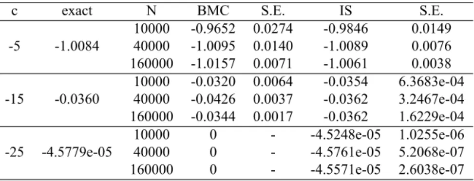
We perform the sampling again, the numerical results are shown below.

Table 3.1: Brownian motion case

c exact N BMC S.E. IS S.E.

10000 -0.9652 0.0274 -0.9846 0.0149 -5 -1.0084 40000 -1.0095 0.0140 -1.0089 0.0076 160000 -1.0157 0.0071 -1.0061 0.0038

10000 -0.0320 0.0064 -0.0354 6.3683e-04 -15 -0.0360 40000 -0.0426 0.0037 -0.0362 3.2467e-04 160000 -0.0344 0.0017 -0.0362 1.6229e-04

10000 0 - -4.5248e-05 1.0255e-06

-25 -4.5779e-05 40000 0 - -4.5761e-05 5.2068e-07

160000 0 - -4.5571e-05 2.6038e-07

T = 30, ρ = 0.7.

Again, we can see that when c =−25, the basic Monte Carlo method cannot sample a rare event even we simulate 160000 times, while the importance sampling method we provide gives an accurate estimation. In addition, the sample error of importance sampling scheme is at least an order smaller than that of basic Monte Carlo method when c < −15.

Chapter 4

Geometric Brownian Motion Case

Let two assets be defined by the following:

dS_it = µ_iS_itdt + σ_iS_itdW_it dS_mt = µ_mS_mtdt + σ_mS_mtdW_mt, where Wit, Wmtare Brownian motion satisfying Wit = ρWmt+√

1− ρ²Zt. Wmt, Ztare independent Brownian motion.

Let r_it = ln_S^Sit

i0, r_mt = ln_S^Smt

m0. In this chapter, we are going to estimate E[r_iT1(r_mT < c)].

4.1 Change measure

It can be derived that

lnS_iT

S_i0 = (µ_i −σ_i²

2 )T + σ_iW_iT lnSmT

S_m0 = (µ_m− σ_m²

2 )T + σ_mW_mT. It means that the event{rmT < c} is equivalent to {WmT < ^c−(µm−

σ2m 2 )T

σm }. Thus, we can again use a similar method as previous chapter. That is, we define

where h is a constant and ˜WmT is a Brownian motion under ˜P . Since we hope that E[r˜ mT] = c, we can get

E[ln˜ SmT

S_m0] = (µ_m−σ_m²

2 )T + σ_mE[W˜ _mT]

= (µ_m−σ_m²

2 )T + σ_mE[ ˜˜ W_mT + hT ]

= (µm−σ_m²

2 )T + σmhT

= (µ_m−σ_m²

2 + σ_mh)

= c, which implies that h = ^c−(µm−

σ2m 2 )T σmT .

4.2 Asymptotic variance analysis

Let ˜c = ^c−(µm−

σ2m 2 )T

σm . Then the first moment is M₁ = E[r_iT1(r_mT < c)]

= E[((µ_i−σ_i²

2 )T + σ_iW_iT)1((µ_m−σ_m²

2 )T + σ_mW_mT < c)]

= (µ_i− σ²_i

2 )T · E[1(WmT < ˜c)] + σ_i· E[WiT1(W_mT < ˜c)]

= (µ_i− σ²_i

2 )T · Φ( ˜c

√T)− ρσ_i√

√ T

2π e^−2Tc2˜ . It implies that

c→−∞lim 1

c² ln|M1|

= lim

c→−∞

1

c²ln|e^−2Tc2˜ ((µ_i− ^σ₂ⁱ²)T√

√ T

2π(−˜c) −ρσi

√T

√2π )|

= lim

c→−∞

1

c²(−[c− (µm−^σ₂^2m)T ]² 2T σ_m² )

=− 1

2T σ²_m.

Before we consider the second moment, we define a new measure ˆP by dP

d ˆP = e^hWmT+12h2T Wˆ_mT = W_mT + hT,

where ˆW_mT is a Brownian motion under ˆP . Then we can calculate the second moment as follows:

M₂ = ˜E[r_iT² 1(r_mT < c)(dP d ˜P)²]

= ˜E[r_iT² 1(r_mT < c)e^h2T−2hWmT]

= e^h2TE[((µˆ i− σ_i²

2 )T + σiWiT)²1(WmT < ˜c)]

= e^h2T{(µi−σ_i²

2 )²T²E[1(Wˆ _mT < ˜c)]

+ 2(µ_i−σ_i²

2 )σ_iT ˆE[W_iT1(W_mT < ˜c)]

+ σ²_iE[Wˆ _iT² 1(W_mT < ˜c)]}

= e^h2T{(µi−σ_i²

2 )²T²E[1(Wˆ _mT < ˜c)]

+ 2(µ_i−σ_i²

2 )σ_iT ρ ˆE[W_mT1(W_mT < ˜c)]

+ σ²_i(ρ²E[Wˆ _mT² 1(W_mT < ˜c)] + (1− ρ²) ˆE[Z_T²1(W_mT < ˜c)])}

= e^h2T{(µi−σ_i²

2 )²T²E[1( ˆˆ W_mT < ˜c + hT )]

+ 2ρ(µ_i− σ²_i

2 )σ_iT ˆE[( ˆW_mT − hT )1( ˆW_mT < ˜c + hT )]

+ ρ²σ²_iE[( ˆˆ W_mT − hT )²1( ˆW_mT < ˜c + hT )] + (1− ρ²)σ_i²T Φ(c + hT˜

√T )}

= e^h2T{(µi−σ_i²

2 )²T²Φ(˜c + hT

√T )

+ 2ρ(µ_i− σ²_i

2 )σ_iT (−

√T

√2πe^{−(˜c+hT )22T} − hT Φ(˜c + hT

√T ))

+ ρ²σ²_iE[( ˆˆ W_mT² − 2hT ˆW_mT + h²T²)1( ˆW_mT < ˜c + hT )]

+ (1− ρ²)σ_i²T Φ(˜c + hT

√T )}

= e^˜c2T{(µi−σ_i²

2 )²T²Φ( 2˜c

√T) + 2ρ(µ_i− σ_i²

2 )σ_iT (−

√T

√2πe^−2˜Tc2 − ˜cΦ( 2˜c

√T))

+ ρ²σ²_i(−2˜c√

√ T

2π e^2˜Tc2 + T Φ( 2˜c

√T) + 2˜c√

√ T

2π e^2˜Tc2 + ˜c²Φ( 2˜c

√T))

+ (1− ρ²)σ_i²T Φ( 2˜c

√T)}

√

It implies that

c→−∞lim 1

c² ln|M2|

= lim

c→−∞

1

c² ln|e^−˜c2T[(µ_i− ^σ₂²ⁱ)²T²√

√ T

2π(−2˜c) + 2ρ(µ_i−σ_i²

2 )σ_iT (−

√T

√2π − c˜√

√ T

2π(−2˜c)) + σ²_i√

√ T

2π(−2˜c)(ρ²c˜²+ T )]|

= lim

c→−∞

1

c²(−[c− (µm−^σ₂^2m)T ]² T σ²_m )

=− 1 T σ²_m.

Thus, we have the following theorem.

Theorem 3. Suppose Wit = ρW_mt+√

1− ρ²Z_t, where W_mt, Z_tare Brownian motion, and ρ is correlation between W_itand W_mt. Define two assets

dS_it = µ_iS_itdt + σ_iS_itdW_it dS_mt = µ_mS_mtdt + σ_mS_mtdW_mt. Also, let

M₁ = E[r_iT1(r_{M T} < c)]

= ˜E[r_iT1(r_{M T} < c)dP d ˜P] M₂ = ˜E[r²_iT1(r_{M T} < c)(dP

d ˜P)²], where

rit = lnS_it

S_i0, rmt = lnS_mt S_m0 Then,

c→−∞lim 1

c² ln|M2| = 2 lim

c→−∞

1

c² ln|M1|.

In summary, we can get a more general theorem, shown as below.

Theorem 4. Let X, Y be random variables such that



X Y



 ∼ N







m₁ m₂



,



 σ²₁ ρσ₁σ₂ ρσ₁σ₂ σ₂²









Also, let

M1 = E[Y 1(X < c)]

M₂ = ˜E[Y²1(X < c)(dP d ˜P)²], where

dP d ˜P = e⁻

(x−m1)2 2σ21

e⁻

(x−c)2 2σ21

. Then,

c→−∞lim 1

c² ln|M2| = 2 lim

c→−∞

1

c² ln|M1|.

Proof. Define a random variable Z such that Y = ρX +√

1− ρ²Z. Then Z ∼ N(m2− ρm1

√1− ρ² ,σ₂²− ρ²σ₁² 1− ρ² ).

Thus,

M1 = ρE[X1(X < c)] +√

1− ρ²E[Z1(X < c)]

= ρ(− σ₁

√2πe⁻

(c−m1)2

2σ21 + m₁Φ(c− m1

σ1

)) +√

1− ρ²m√₂− ρm1

1− ρ² Φ(c− m1

σ1

)

=−ρ σ1

√2πe⁻

(c−m1)2

2σ21 + m₂Φ(c− m1

σ₁ ).

Since

Φ(c− m1

σ₁ )≈ √ −σ1

2π(c− m1)e⁻

(c−m1)2

2σ21 as c→ −∞, we can derive that

c→−∞lim 1

c² ln|M1| = − 1 2σ₁². On the other hand,

M₂ = ˜E[(ρ²X²+ 2ρ√

1− ρ²XZ + (1− ρ²)Z²)1(X < c)(dP d ˜P)²]

= ρ²e

(c−m1)2

σ21 [−2σ₁m₁

√2π e⁻

2(c−m1)2

σ21 + (σ₁²+ (c− 2m1)²)Φ(2c− 2m1

σ1

)]

+ 2ρ(m₂− ρm1)e

(c−m1)2

σ21 (− σ₁

√2πe⁻

2(c−m1)2

σ21 − (c − 2m1)Φ(2c− 2m1

σ₁ ))

we can derive that

c→−∞lim 1

c²ln|M2| = − 1 σ²₁. Therefore,

c→−∞lim 1

c² ln|M2| = 2 lim

c→−∞

1

c² ln|M1|.

Remark. Theorem 1, Theorem 2, Theorem 3 are the special cases of Theorem 4.

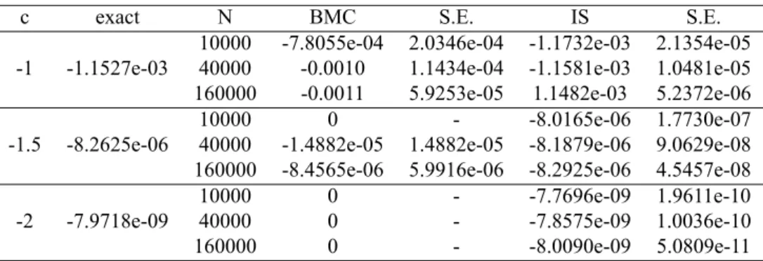
4.3 Numerical results

We show the numerical results again. The results are shown below.

Table 4.1: Geometric Brownian motion case

c exact N BMC S.E. IS S.E.

10000 -7.8055e-04 2.0346e-04 -1.1732e-03 2.1354e-05 -1 -1.1527e-03 40000 -0.0010 1.1434e-04 -1.1581e-03 1.0481e-05 160000 -0.0011 5.9253e-05 1.1482e-03 5.2372e-06

10000 0 - -8.0165e-06 1.7730e-07

-1.5 -8.2625e-06 40000 -1.4882e-05 1.4882e-05 -8.1879e-06 9.0629e-08 160000 -8.4565e-06 5.9916e-06 -8.2925e-06 4.5457e-08

10000 0 - -7.7696e-09 1.9611e-10

-2 -7.9718e-09 40000 0 - -7.8575e-09 1.0036e-10

160000 0 - -8.0090e-09 5.0809e-11

T = 0.5, µi= 0.08, σi= 0.3, Si0= 10, µm= 0.1, σm= 0.5, Sm0= 100, ρ = 0.7.

Here we can see that when c = −2, the basic Monte Carlo method cannot sample a rare event even we simulate 160000 times, while the importance sampling method we provide gives an accurate estimation. In addition, the sample error of importance sampling scheme is at least an order smaller than that of basic Monte Carlo method.

Chapter 5

Applications to Measuring Systemic Risk

After the 2008 financial crisis, measuring systemic risk has become a crucial issue for the financial stability. Governments are trying to figure out why the regulation failed, how much capital is required and how to address the next financial crisis. Bisias et al. [10] pro- vide a survey on the systemic risk measures and conceptual frameworks that have been developed in the past few years. There are some measures that are widely adopted, such as SRISK and ∆CoVaR. Adrian and Brunnermeier (2011) allow for tail dependence and use a quantile regression approach to estimate the ∆CoVaR. Brownlees and Engle (2012) model time-varying linear dependencies and use a multivariate GARCH-DCC model to compute the SRISK.

In this chapter, we will estimate the systemic risk measurement SRISK in the framework of Stochastic Volatility Model(SV model). SRISK is defined as the expected capital shortfall of a financial entity conditional on a prolonged market decline. SRISK can be considered to be a function of several variables. One of these variables is Long Run Marginal Ex- pected Shortfall(LRMES). Our goal is to estimate LRMES using the Monte Carlo method and compare it with the importance sampling method.

5.1 Stochastic Volatility model

and assume that stochastic correlation follows Jacobi process.

The overall model is constructed below:













































d ln Smt = (µm− ^Vmt₂ )dt +√

VmtdWmt

dV_mt = κ_m(θ_m− Vmt)dt + ξ_m√

V_mtdZ_mt d ln S_it = (µ_i− ^V₂^it)dt +√

V_itdW_it dV_it = κ_i(θ_i− Vit)dt + ξ_i√

V_itdZ_it d⟨Wm, Z_m⟩t = ρ_mdt

d⟨Wi, Z_i⟩t = ρ_idt d⟨Wm, W_i⟩t = ρ_itdt

dρit = αi(mi− ρit)dt + βi

√1− ρ²itdXit

where S_mt, S_itdenote the market index and stock price of the i-th firm, respectively, and V_mt, V_it are the corresponding stochastic volatility. W_mt, W_it, Z_m, Z_i, X_it are the stan- dard Brownian motions, where ρ_m, ρ_i, ρ_itare correlations between each Brownian motion.

κm, κi are the mean reverting speed of corresponding volatility. θm, θi are the long-run level of the volatility. ξm, ξi are the volatility of volatility. αi represents the mean recov- ery rate. β_i represents the volatility.

Define the i-th firm’s LRMES from time t to time t + h by

LRMES_i,t:t+h=−E[ri,t:t+h(t + h)|Crisist:t+h]

=−E[r_i,t:t+h(t + h)1(r_m,t:t+h(t + h) < c)]

E[1(r_m,t:t+h(t + h) < c)] , (5.1) where r_m,t:t+h and r_i,t:t+h are the returns of index of market and the i-th firm over the period [t, t + h].

Sometimes the ”Crisis” is a rare event, depending on the value of c. If it is a rare event, then we will introduce the importance sampling method to reduce sample variance. Otherwise, the basic Monte Carlo method is enough.

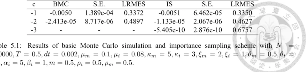
The numerical results are presented in the following table.

c BMC S.E. LRMES IS S.E. LRMES -1 -0.0050 1.389e-04 0.3372 -0.0051 6.462e-05 0.3350 -2 -2.413e-05 8.717e-06 0.4897 -1.133e-05 2.067e-06 0.4627

-3 - - - -5.405e-10 2.876e-10 0.6757

Table 5.1: Results of basic Monte Carlo simulation and importance sampling scheme with N = 160000, T = 0.5, dt = 0.002, µm = 0.1, µi = 0.08, κm = 5, κi = 3, ξm = 2, ξi = 1, θm = 0.5, θi = 0.3, α_i= 5, β_i= 1, m = 0.5, ρ_i= 0.5, ρ_m= 0.5.

From the numerical results, we can see that the basic Monte Carlo method doesn’t work well when c is very small. On the other hand, the standard error was reduced when we use the importance sampling method.

5.2 First Passage Time Case

In this section, we introduce another definition of LRMES. It is called the first passage time problem, or the hitting time problem. We will also use the Heston model, but here we define LRMES as follows:

LRMES_i,0:T =−E[ri,0:T(T )|Crisis0:T]

=−E[r_i,0:T(T )1(inf_ur_m,0:T(u) < c)]

E[1(inf_ur_m,0:T(u) < c)] . (5.2) The only difference between (5.1) and (5.2) is the ”Crisis” event. Here we define the ”Cri- sis” to be the minimum market return below c during the time [0, T ]. Before we show the numerical results, we need to show how to compute the denominator and the numerator of LRMES under the constant volatility model. More specifically, we need to derive the density function.

Let ˆW_mt = αt + W_mt, where W_mt is a standard Brownian motion. Define ˆm(T ) = min_0≤t≤TWˆ_mt, then we can derive the joint distribution of ˆm(T ) and ˆW_mt. Then deriva- tion is similar to [6]. Let ˆZ(t) = e^{−αWmt−12α2t} = e^{−α ˆWmt+12α2t}. By Girsanov’s Theorem, Wˆ_mtis a Brownian motion under the measure ˆP . By using a similar derivation in [6], we

Hence,

P ( ˆm(T )≤ m, ˆW_mT ≤ w) = E[1( ˆm(T )≤ m, ˆW_mT ≤ w)]

= ˆE[ 1

Z(T )ˆ 1( ˆm(T )≤ m, ˆW_mT ≤ w)]

= ˆE[e^{α ˆWmT−12α2T}1( ˆm(T )≤ m, ˆW_mT ≤ w)]

=

∫ _w

−∞

∫ _m

−∞

e^αy−12α2Tfˆ_{m(T ), ˆˆ W}

mT(x, y)dxdy.

Therefore, under the measure P , f_{m(T ), ˆˆ W}

mt(x, y) =−2(2x− y) T√

2πT exp(αy− 1

2α²T −(2x− y)²

2T ), x < 0, y ≥ x.

Let α = _σ¹

m(µ_m− ¹₂σ_m²) and ˆc = _σ^c

m. Then we can see that

S_mt= S_m0e^{σmWmt+(µm−12σ2m)t}

= S_m0e^σmWˆmt. Hence, we can get the denominator

E[1(inf_ur_m,0:T(u) < c)]

= E[1(inf_ulnSmu

S_m0 < c)]

= E[1(inf_uWˆ_mu< ˆc)]

=

∫ _ˆc

−∞

∫ _∞

x

f_{m(T ), ˆˆ W}

mt(x, y)dydx

=

∫ ˆc

−∞

∫ y

−∞−2(2x− y) T√

2πT e^{αy−12α2T−(2x−y)22T} dxdy +

∫ _∞

ˆ c

∫ _ˆc

−∞−2(2x− y) T√

2πT e^{αy−12α2T−(2x2T−y)2}dxdy

= e^2αˆcΦ(ˆc + αT

√T ) + Φ(ˆc− αT√ T )