國立臺灣大學工程學院化學工程學系 碩士論文
Department of Chemical Engineering College of Engineering
National Taiwan University Master Thesis
最佳化批次結晶程序之目標函數選擇
Comparison of objective functions for seeded batch crystallization
許哲維 Che-Wei Hsu
指導教授:吳哲夫 博士 Advisors: Jeffrey D. Ward, Ph.D.
中華民國 100 年 7 月
July, 2011
i
致謝 致謝 致謝 致謝
首 先 在 此 由 衷 的 感 謝 吳 哲 夫 教 授 這 兩 年 的 付 出 , 特 別 是 在 余 政 靖 教 授 剛 過 世 時 , 實 驗 室 一 片 混 亂 的 情 況 下 接 下 了 團 隊 並 指 導 。 另 外 也 感 謝 陳 誠 亮 教 授 、 錢 義 隆 教 授 、 黃 孝 平 教 授 與 蕭 立 鼎 教 授 對 於 研 究 的 指 導 。
在 這 兩 年 的 研 究 期 間 , 感 謝 同 屆 的 朋 友 ( 雨 利 、 冠 安 、 承 勳 、 翊 軒 、 信 杰 、 少 儂 ) 在 修 課 和 研 究 之 餘 的 陪 伴 。 感 謝 實 驗 室 曾 經 指 導 過 我 的 學 長 姐 ( 愛 真 、 建 凱 、 乾 元 、 玉 龍 、 愷 悌 、 雅 玲 ) 和 同 實 驗 室 的 同 事 們 ( 郁 迪 、 傳 真 、 均 彥 、 孟 達 、 育 賢 、 鎮 宇、宗 翰 ),最 後 感 謝 實 驗 室 的 學 弟 妹 ( 偉 倫、紹 群、騰 雲 ) 。
ii
緒論 緒論 緒論 緒論
結 晶 是 一 個 常 被 用 來 作 為 液 態 固 態 分 離 的 程 序 。 而 一 個 結 晶 槽 的 成 品 可 以 用 結 晶 大 小 分 佈 函 數 ( C r y s t a l S i z e D i s t r i b u t i o n F u n c t i o n , C S D ) 來 描 述 。 成 品 的 好 壞 將 影 響 下 游 程 序 的 效 率 , 例 如 過 濾 或 是 乾 燥 程 序 。 在 結 晶 的 過 程 中 , 同 時 會 出 現 結 晶 成 核 ( c r y s t a l n u c l e a t i o n ) 與 結 晶 成 長 ( c r y s t a l g r o w t h ) 現 象 , 在 大 多 數 的 情 況 下 結 晶 成 核 現 象 是 不 受 歡 迎 的 。 一 個 控 制 得 好 的 結 晶 槽 , 可 以 有 效 抑 制 結 晶 成 核 現 象 的 發 生 。
要 最 佳 化 一 個 結 晶 程 序 可 以 從 兩 方 面 來 著 手 , 一 種 是 改 善 晶 種 的 性 質 , 另 一 種 是 改 善 冷 卻 的 方 法 。 而 不 管 是 使 用 哪 一 種 手 段 , 都 需 要 一 個 目 標 函 數 來 評 斷 結 果 的 好 壞 。 在 這 個 研 究 中 , 我 們 比 較 前 人 在 這 個 領 域 上 使 用 過 的 目 標 函 數 , 希 望 能 夠 發 現 一 個 最 適 合 的 目 標 函 數 。
在 使 用 各 個 目 標 函 數 後 , 我 們 發 現 有 些 目 標 函 數 的 結 果 藉 由 產 生 大 量 的 成 核 現 象 以 達 到 其 目 標 函 數 值 的 最 小 值 。 但 以 一 個 先 加 入 晶 種 的 結 晶 程 序 而 言 , 其 目 標 是 將 晶 種 長 大 並 避 免 成 核 現 象 的 發 生 , 前 述 達 到 其 目 標 函 數 值 的 方 法 是 與 其 牴 觸 的 。 事 實 上 在 真 實 的 程 序 裡 , 在 結 晶 之 後 很 有 可 能 經 過 一 個 過 濾 的 程 序 將 過 小 的 晶 體 或 是 新 成 核 的 晶 體 移 除 。 所 以 對 於 各 個 不 同 的 目 標 函 數 , 我 們 除 了 直 接 比 較 用 其 最 佳 化 的 結 果 的 目 標 函 數 值 以 外 , 也 比 較 新 成 核 晶 體 被 移 除 後 的 目 標 函 數 值 。 最 後 我 們 發 現 使 用 目 標 函 數 ” 最 小 化 新 成 核 晶 體 的
iii
質 量 ” 來 最 佳 化 , 其 結 果 在 新 成 核 晶 體 被 移 除 後 , 對 於 各 個 目 標 函 數 值 都 有 較 佳 的 值 。
對 於 目 標 函 數 ” 最 小 化 結 晶 分 佈 函 數 的 變 異 係 數 ” , 我 們 發 現 與 其 最 佳 化 結 晶 成 長 曲 線 , 使 用 晶 種 性 質 作 為 控 制 變 數 有 較 佳 的 效 果 。 較 大 量 的 晶 種 質 量 與 較 集 中 的 晶 種 分 佈 , 在 使 用 ” 最 小 化 結 晶 分 佈 函 數 的 變 異 係 數 ” 作 為 目 標 函 數 時 , 將 有 效 防 止 大 量 成 核 現 象 的 發 生 。
最 後,我 們 探 討 結 晶 成 核 速 率 式 中,在 晶 體 體 積 項 ( T h i r d M o m e n t ) 較 高 的 幕 次 對 於 最 佳 化 程 序 的 影 響 。 我 們 發 現 , 較 高 的 幕 次 將 抑 制 成 核 現 象 的 發 生 , 造 成 最 佳 化 的 結 果 有 較 佳 的 表 現 。 另 外 較 高 的 幕 次 也 將 使 得 最 佳 化 晶 體 成 長 曲 線 在 程 序 的 一 開 始 有 較 高 的 值 。
iv
Abstract
Crystallization is a widely used process for liquid solid separation. The products from this process are crystals, which can be described by a distribution function called “crystal size distribution function (CSD)”. The properties of the crystals affect the efficiency of downstream process, such as filtration or drying. During the process both crystal nucleation and crystal growth happens, and most of the time, the crystal nucleation is undesirable. A well-controlled crystallizer can produce crystals with less crystal nucleation.
Researchers have optimize a crystallization processes by improving the seed properties or the cooling policy. In both cases an objective function is required. In this work we compare the objective function that researchers have used, to see which objective function is best when optimizing the cooling policy for a batch crystallizer.
The result shows that some of the objective functions are minimized by producing a large amount of nuclei. However, for a seeded batch crystallizer the idea is to grow the seed crystals while suppressing the nucleation.
Moreover, in industrial practice, the product crystals would probably be filtered so that fines (nucleated crystals) would be removed. Therefore, for each objective function we also determine the objective value after the
v
nucleated crystals are removed, to see whether the result from each objective function is still the best. After the analysis we conclud that the objective function “minimizing the nucleated crystal mass” is better than others.
In this work we also discuss the utility of changing seed properties when using “minimizing weight coefficient of variation” as objective function. We found that if the seed distribution is too wide, the system would be more likely to generate a narrow distribution crystal by excess nucleation. To prevent excess nucleation and achieve a narrow product CSD, a large seed loading and a narrow seed distribution helps.
Finally, we also considered the effect of using different nucleation parameters. We changed the exponent on third moment term in nucleation rate equation. The result shows that for higher value of the exponent, the nucleation rate is suppressed, and the performance is better when the growth rate trajectory is optimized using the objective function “minimizing nucleated crystal mass.” The optimized result also mention that for higher value of the exponent on third moment term in nucleation rate equation, higher growth at the beginning of the batch is desirable.
vi
Table Of Content
List Of Figures ... viii
List Of Tables ... xii
1. Introduction ... 1
1.1. Overview ... 1
1.2. Literature Survey ... 4
2. Dimensionless Model ... 8
2.1. Dimensionless Moment Equations ... 8
2.2. Seed ... 12
3. Optimization by Simulated Annealing ... 15
1.1. Simulated Annealing ... 15
4.1. Control Variable ... 22
4.2. Final Mass Constraint ... 22
4. Discussion ... 24
4.1. Objective Function Classification ... 24
4.2. Comparison Method ... 27
vii
4.3. Weight COV and Number COV ... 29
4.5. Single Moment Objective Functions ... 44
4.6. Objective Function Category Comparison ... 51
4.7. Other Solution For Minimizing Coefficient of variation ... 57
4.8. The Effect of Changing j ... 63
5. Conclusion ... 73
6. Notations... 75
7. Reference ... 77
viii
List Of Figures
Figure 1: Supersaturation and metastable zone. [1] ... 2
Figure 2: The parabolic seed crystal size distribution (CSD) function. ... 12
Figure 3: Representation of optimization by simulated annealing. ... 17
Figure 4: The annealing temperature. ... 18
Figure 5: Simulation annealing algorithm. ... 21
Figure 6: Final crystal size distribution for different objectives. ... 29
Figure 7: The optimal growth trajectory using objective function, minimizing weight coefficient of variation and minimizing number coefficient of variation. ... 30
Figure 8: The optimal nucleation rate trajectory using objective function, minimizing weight coefficient of variation and minimizing number coefficient of variation. ... 31
Figure 9: Weight coefficient of variation and number coefficient of variation value for different objectives. ... 32
Figure 10: The optimal concentration trajectory using objective function, minimizing weight coefficient of variation and minimizing number coefficient of variation. ... 34
ix
Figure 11: Different order of moment plot during the batch time for using
objective function minimizing weight coefficient of variation and
minimizing number coefficient of variation. ... 35
Figure 12: The optimal nucleation rate trajectory using objective function, minimizing weight mean size and minimizing number mean size. ... 36
Figure 13: The optimal growth trajectory using objective function, minimizing weight mean size and minimizing number mean size. ... 37
Figure 14: The optimal concentration trajectory using objective function, minimizing weight mean size and minimizing number mean size. ... 38
Figure 15: Different order of moment plot during the batch time for using objectives function minimizing weight mean size and minimizing number mean size. ... 40
Figure 16: Weight mean size and number mean size value for different objectives. ... 42
Figure 17: Final crystal size distribution for different objectives. ... 43
Figure 18: Nucleated crystal moments of for different objectives. ... 45
Figure 19: Seeded crystal moments for different objectives. ... 46
Figure 20: Final crystal size distribution for different objectives. ... 47
x
Figure 21: Different order of moments during the batch using minimizing µ ,n0
1
µ ,n µ and n2 µ as objective function. ... 49n3 Figure 22: The optimal nucleation rate trajectory using minimizingµ ,n0 µ ,n1 µn2
and µ as objective function. ... 50n3 Figure 23: The optimal growth rate trajectory using minimizingµ ,n0 µ ,n1 µ and n2
3
µ as objective function. ... 50n
Figure 24: The optimal growth trajectory using minimizing µ , weight n3
coefficient of variation and maximizing weight mean size. ... 52 Figure 25: The optimal nucleated trajectory using minimizing µ , weight n3
coefficient of variation and maximizing weight mean size. ... 52 Figure 26: The optimal concentration trajectory using minimizing µ , weight n3
coefficient of variation and maximizing weight mean size. ... 53 Figure 27: Different moments during the batch using minimizing µ , weight n3
coefficient of variation and maximizing weight mean size. ... 54 Figure 28: Weight mean size, weight coefficient of variation and third moment
values for different objectives. ... 55 Figure 29: Final crystal size distribution for different objectives. ... 56
Figure 30: Initial crystal size distribution which is used for minimizing weight
coefficient of variation result. ... 58
xi
Figure 31: The growth trajectory for different seed distribution width which is
used for minimizing weight coefficient of variation result. ... 59
Figure 32: Final crystal size distribution for minimizing weight coefficient of variation. ... 61
Figure 33: The concentration trajectory for different seed distribution width which is used for minimizing weight coefficient of variation result. ... 62
Figure 34: The growth rate for different j. ... 66
Figure 35: The concentration trajectory for different j value. ... 70
Figure 36: Final crystal size distribution for different j value. ... 71
Figure 37: Different moment during the batch for different j value. ... 72
xii
List Of Tables
Table 1: Parameters that for simulated annealing ... 20
Table 2: Objective functions used from literature. ... 25
1
1. Introduction
1.1. Overview
Crystallization is a widely used solid liquid separation process. It occurs when the solute concentration exceed the saturate concentration. We define the supersaturation as the difference between the solute concentration and the saturated solute concentration. The supersaturation can be made by cooling the system, evaporating the solvent from system or adding compound that decreases the saturation concentration of the solute. When in process, the supersaturation usually is controlled in metastable region. The metastable region is shown in Figure 1. When the supersaturation is under metastable region, the crystal starts to dissolve. On the other hand, when the supersaturation exceeds the metastable region, a large amount of nucleation would occur.
3
the suspend crystal exists. In this work, the batch process starts with seed crystal. So the secondary nucleation is the major nucleation mechanism.
Another phenomenon is crystal growth. The crystal growth will increase the size of the crystal, both seeded crystal and nucleated crystal. In reality, if the supersaturation is increasing, both nucleation rate and growth rate would increase. But the magnitude of increase for nucleation rate is larger than growth rate. Therefore, if we want to suppress the nucleation rate when keeping the crystal growth, we can keep the supersaturation value low in entire process. However, if we do so, the entire process would take too much time.
A good process is to produce desired crystal size distribution (CSD), because it is not only the quality of the product, but also influences the efficiency of the downstream process like filtration or drying. However, there are different ways to evaluate how good the product CSD is due to different situation. Researchers use different objective functions to optimize the process for different needs of the process. These objective functions are things to be focus in this work.
4
1.2. Literature Survey
Batch crystallization is a widely used liquid sold separation process. The system can be described by mass balance and population balance. After the work of Jones (1974) [2], many researchers use moment transformation to study this system. Ward et al. developed a dimensionless model based on moment transformation, which helps to develop an imperial concept that is not specific to any solute-solvent system.
There are two ways to optimize a batch crystallizer. One is by optimizing the seeding (Kubota and Doki et al. [3], Lung-Somarriba et al. [4], Hojjati and Rohani [5] and Chung et al. [6]). Another way is optimizing the temperature trajectory. At 1974, Jones et al.[2] compare the result from nature cooling, linear cooling and constant nucleation rate cooling and conclude that controlled cooling significantly reduce the nucleation and enlarger the larger crystal.
Due to the high non-linearity of the crystallization mathematical model, pioneer researcher developed some approximate trajectory instead of optimizing the temperature. Mullin and Nyvlt[7] developed a trajectory based on the assumption of negligible nucleation and constant supersaturation, it has a great advantage that the trajectory can be determined with only the mass of the seed, the initial and final concentration and the batch time. Chung et al. [6]
5
optimize both the temperature trajectory and the seeding parameters with dynamic programming framework. Ward et al.[9] optimized the growth trajectory (supersaturation profile) by sequentially iteration. However, due to the convex nature of the system, when using different objective functions, the system may not converge. Moreover, with different initial guesses, sometimes the system will converge to a local minimum. Choong et al.[8], applied simulated annealing for the optimization of crystallization systems. This method is widely used for non-linear systems. Simulated annealing is also being known as a method that can often find the global minimum in non-convex problems. It is the optimization strategy used in this work.
Some researchers consider multiple objective function, usually combing them into one objective using a weighted sum. For example, when the goal is to minimize both weight mean size of the crystal and the mass of the nucleated crystal, the objective function may become “minimizing weight mean size plus mass of the nucleated crystal.” In this example the weighting factor for the weight mean size and the mass of the nucleated crystal both is one. If minimizing mass of the nucleated crystal is more important, weighting factor for it would be higher than other. Then the problem is to determine the weighting factor for each objective.
6
Another approach for consider multiple objectives is to determine the so-called Praeto-optimal front. Sarkar et al.[24] proposed to use genetic algorithm to solve these kind of multi objective function problem. They use genetic algorithm to generate an optimal solution set with a Praeto-front. Once the Praeto-optimal solution is achieved, the user can visualize the trade-off between objectives and choose an operate point. However, when it comes to three objective functions or more, it is hard to visualize the optimal solution from Praeto-optimal solution figure. Furthermore because the genetic algorithm is mapping through different weighting factors of objective functions, it cost more time than solving the problem using a single objective function.
One objective function may correlate closely with another objective function. For example, optimize with objective function “minimizing mass of the nucleated crystals” would achieve a similar result as using the objective function “maximizing weight mean size of the crystals.” That is because the general goal of these two objective functions is suppressing nucleation. In reality, nucleated crystals are undesirable. Most objective functions considered in the literature are concerned with suppressing the nucleation. In this work, we are collect the objective function that have been used by and compare them by comparing the results of using each objective function. The goal is to see
7
whether there is one single objective function that works well for many purposes.
8
2. Dimensionless Model
2.1. Dimensionless Moment Equations
Without agglomeration and breakage, for a well-mixed batch crystallizer, the population balance can be expressed like this:
( )
,( ( ) ( )
, ,)
G L t f L t 0 f L t
t L
∂ ∂
+ =
∂ ∂ (1)
Where f L t( , ) is the crystal size distribution (CSD) function, B (#/m3s) and G (m/s) are nucleation rate and growth rate, respectively. A left boundary condition could be applied:
( ) ( ( ) )
( )
, ,
0, 0,
B f L t t f t
G t
= (2)
Here is the definition of moments of CSD:
( )
0
0,1, 2,...
i
i L f L dL i µ
∞
=
∫
= (3)A population balance equation with moments can be shown like this:
d 0
dt B
µ = (4)
1 1,2,...
i
i
d iG i
dt
µ = µ− = (5)
The nucleated crystals (subscript n) and the seed-grown crystals (subscript s) are tracked individually. The population moment equation for the seed-grown crystal can be described like this:
9
,0 0
d s
dt
µ = (6)
,
, 1 1, 2,...
s i
s i
d iG i
dt
µ = µ − = (7)
And for the nucleated crystal:
,0
d n
dt B
µ = (8)
,
, 1 1, 2,...
n i
n i
d iG i
dt
µ = µ − = (9)
The crystallization process is driven by supersaturation. It is the difference of current concentration and saturated concentration.
S= −C Csat (10)
The concentration can be measured by mass balance.
3 c v 3
dC G k
dt = − ρ µ (11)
Where ρc is the crystal density and kv is the crystal volumetric shape factor. A common expression for crystal growth rate and secondary nucleation
rate are:
g
G =k Sg (12)
3
B=k Gb γµ (13)
where kg , g , kb and γare kinetic parameters. To generalize the analysis,
the equations from 4 to 11 are non-dimensionalized.
We define:
10
0 f
f
C C C C C
′ = −
− (14)
t′ =t tf (15)
Where tf is the total batch time, and C’ is the dimensionless
concentration which decreases from 1 to 0 during the batch. We also define the dimensionless G and B
G G
′ =G (16)
( )
b f4 13G k t γ
−
= + (17)
( )
4 33
b b f
B B
B B
k k t
γ
µ γ−+
′ = = (18)
( )
4 33
b b f
B k k t
γ
µ γ−+
= (19)
From the concept of mass balance, we define:
3 3
3
µ µ
′ = µ (20)
( )
† 0 0 3
f
c v c v
C C
C
k k
µ ρ ρ
= = − (21)
To simplify Equation 5, we also define:
0 Btf
µ = (22)
2 1 BG tf
µ = (23)
2 3
2 BG tf
µ = (24)
3 4
3 BG tf
µ = (25)
11
The differential equations becomes:
( )
0
( 3)
d B G
dt µ γ
′ µ
′ ′ ′
= =
′ (26)
1
0
d G
dt
µ′= ′ ′µ
′ (27)
2
2 1
d G
dt
µ′ = ′ ′µ
′ (28)
3
3 2
d G
dt
µ′ = ′ ′µ
′ (29)
13
In order to reach the total mass of the seeds ms, the variable a must satisfy this condition:
( )
0( )
0
2
3 3
0 0
0 2
x w
s
v
x w
L f L L f L m ρk
∞ +
−
= =
∫ ∫
(31)Where ms is the mass of seeds, ρ is density of crystal, kv is shape
factor. Solving the equation we get:
1
3 3 5
0 0
1 1
6 40
s c v
a m x w x w
ρ k
−
= + (32)
Therefore:
( )
3 3 5 10 0 0 0 0
1 1
6 40 2 2
s c v
m w w
f L x w x w L x L x
ρ k
−
= − + − − − + (33)
for x0−w 2≤ ≤L x0 +w 2 .
Define:
0 s s
f
m m
C C
′ = − (34)
0 0
f
x x
′ = Gt (35)
f
L L
′ = Gt (36)
14
f
w w
′ =Gt (37)
( ) ( )
,, Gf L t f L t
′ = B (38)
Substituting the definitions of dimensionless relationship into Equation 33, we will get:
( )
3 3 5 10 0 0 0 0
1 1
6 40 2 2
s
w w
f L m x w x w L x L x
− ′ ′
′ ′ = − ′ ′ ′ + ′ ′ ′− ′− ′− ′+ (39)
From the definition of the moments from Equation 3, the dimensionless moments of seed CSD are given by:
( ) ( )
,0 2 2
0 0
0 20
20 3
s s
m
x x w
µ′ = ′
′ ′ + ′ (40)
( ) ( )
,1 2 2
0
0 20
20 3
s s
m
x w
µ′ = ′
′ + ′ (41)
( ) ( )
( )
2 2
0 0
,2 2 2
0
20
0 20 3
s s
m x w x
x w
µ′ = ′ ′ + ′ ′
′ + ′ (42)
,3
( )
0s ms
µ′ = ′ (43)
At the end of the batch, the total third moment (including the seed crystals and nuclei) of the CSD is:
( ) (
0)
3
s f
f
c v
m C C
t k
µ ρ
+ −
= (44)
( ) ( )
03
3 0
3 ( )
( ) 1
f s f
f
f s
t m C C
t C m
C µ µ
µ
+ −
′ = ′
= = − + (45)
15
3. Optimization by Simulated Annealing
Stimulated annealing is a widely used optimization strategy for non-linear systems. It has the advantage that is the re-annealing mechanism, which helps to find the global minimum. In this work, all of the optimization is done using the stimulated annealing toolbox in MATLAB.
1.1. Simulated Annealing
Simulated annealing is a method that emulates the annealing of metal.
When annealing a metal, the metal is heated and melted. The high temperature gives energy to the metal atoms so that they can move in the metal. After the heating, the metal is cooled. If the cooling rate is fast, defects may form. In nature a defect means a higher energy state. If the cooling rate is slow, then there is more chance for the atoms to arrange more into a lower-energy structured crystal. A well-formed lattice structure means that the metal is in lower energy state. The entire heating and cooling process make the metal change the arrangement from higher energy state to lower energy state.
To develop an analog to the physical annealing, a variable Ta is defined that mimics the physical temperature. The annealing temperature affects two aspects of the simulation. One is the changing of the point. At higher annealing
16
temperature, the distance between current and next tried point will be larger.
Another one is the likelihood of accepting a higher energy state. At higher temperature, the system will be more likely to accept a state with higher objective value.
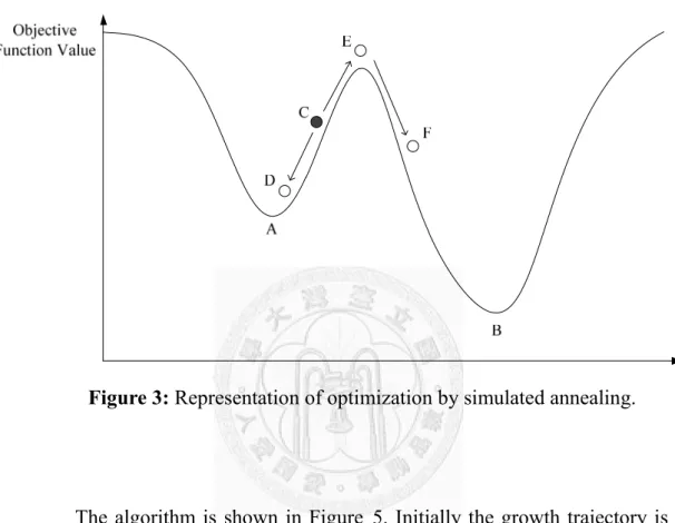
Simulated annealing is widely used because of its ability to avoid local minima. As shown in Figure 3, the vertical axis is the objective function value.
There is a local minimum here shown as point A, and there also is a global minimum shown as point B. The current state is point C. In a traditional minimum finding algorithm, there is no mechanism to accept a worse result.
That means that from the current state point C, the algorithm can only move downward. It will find a minimum value, but the minimum is a local minimum.
The initial guess becomes very important. If the initial guess is near the global minimum, then the result may the global minimum. Otherwise, the algorithm would find a local minimum. By contrast, the simulated annealing algorithm has a mechanism to accept a worse result. As shown in Figure 3, both simulated annealing algorithm and other algorithm will accept point D, because it has lower objective function value. However, point E has an undesirable higher objective function value. In the simulation annealing algorithm there is a
17
possibility to accept point E, and it depends on the current annealing temperature. Once the state reaches the hill at point E, the algorithm then has a chance to reach point F and then the global minimum point B.
Figure 3: Representation of optimization by simulated annealing.
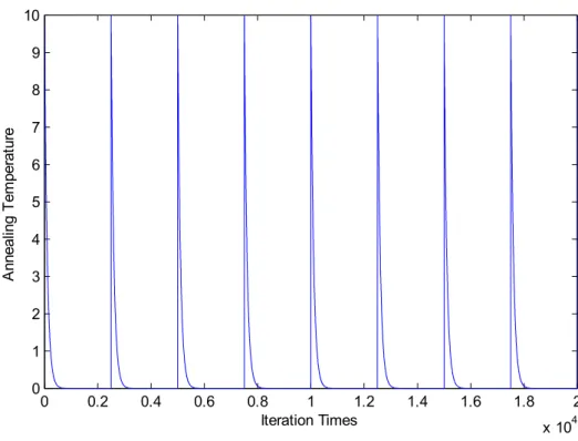
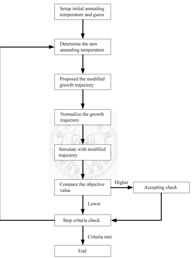
The algorithm is shown in Figure 5. Initially the growth trajectory is a random function provided by MATLAB. The initial annealing temperature we use is 10. The next step is to determine the annealing temperature at the iteration time. The annealing temperature is a function of iteration time (ksa). In
this work, the annealing temperature function can be express by:
( sa) 0.99 ^ mod( sa, )
a ini r
T k =T × k k (46)
18
Where “mod “ is the modulus function, and kr is the number of iterations until the temperature goes back to initial temperature (Tini). A plot of the annealing temperature versus time is shown in Figure 4 for k =r 2500.
Figure 4: The annealing temperature.
The reason of choosing this kind of annealing temperature is that although the code from MATLAB has a re-annealing mechanism to make the algorithm jump out of the local minimum, it is still not enough. So we don’t use the default annealing function but instead construct an annealing temperature profile that reheats the system after kr iterations.
0 0.2 0.4 0.6 0.8 1 1.2 1.4 1.6 1.8 2
x 104 0
1 2 3 4 5 6 7 8 9 10
Iteration Times
Annealing Temperature
19
After the new annealing temperature is determined, as shown in Figure 5, we propose a new growth trajectory according to the annealing temperature.
The higher the annealing temperature, the larger the changing between new trajectory and previous trajectory. The next step is to normalize the growth trajectory such that at the end of the batch, the value of the third moment (µ'3) equal to m +'s 1, according to the mass constraint.
With the new growth trajectory we can run the batch to determine the final crystal moments and the objective function value. The next step is to compare the objective function value from new growth trajectory and previous growth trajectory. There will be two situations: the new objective value may be higher or lower than the previous one. Our goal is to minimize the objective function, so if the objective value from new growth trajectory is lower than the previous one, we accept it with no doubt. On the other hand, if the new objective value is higher than the previous one, it still may be accepted. In the code provided in the MATLAB toolbox, the possibility of acceptance equation is like this:
( ) 1
1 exp
a
P t
T
= ∆
+
(47)
20
Where ∆ is the difference between previous and new objective function value. It is a positive value. Ta is the annealing temperature. The possibility of acceptance is between 0 and 0.5. Larger ∆ value will cause smaller acceptance possibility. If the new growth trajectory is rejected, the program will keep the previous growth trajectory for the next run.
The stop criterion is defined by the iteration time. We set the maximum number of iteration to 30000, the program will give the result and end after the iteration times is over 30000. Table 1 shows the parameters we used for the code provided from MATLAB in this work. For parameter that are not listed in this table, the default setting is used.
Table 1: Parameters that for simulated annealing
Parameter Value
Lower bound 0
Upper bound 100
Initial temperature 10
Temperature function Equation 46 Reannealing interval 300
Maxiter 30000
21
Figure 5: Simulation annealing algorithm.
22
4.1. Control Variable
In this work the control variable is the growth trajectory (G t'( ')). There are two reasons that we do not use the temperature trajectory as the control variable. One is that using temperature trajectory as control variable makes finding a solution more difficult. Another reason is that solubility parameters are required to determine the relationship between temperature trajectory and growth trajectory. If we need the solubility parameters, the result is no longer general to many different systems.
After the optimal growth trajectory is found, the optimal supersaturation trajectory can be determined using Equation 12. We can also find the concentration trajectory by mass balance. Combining the supersaturation and the concentration trajectory we can achieve the saturated concentration trajectory. Appling the solubility parameters to the saturated concentration trajectory, we can have the temperature trajectory.
4.2. Final Mass Constraint
In this work the initial concentration and the final concentration are fixed.
To ensure the final concentration to be the same after every simulation, a
23
constraint is added. From mass balance, the solution concentration directly related to the mass of the crystal in the batch crystallizer. And for the dimensionless model, this constraint make the value of the third moment (µ'3) to be m +'s 1 at the end of the batch, as shown in Equation 44 and Equation 45.
During the simulation, we define the growth trajectory like this:
( ) 0
G t =G ×aa (48)
where G t( ) is growth rate trajectory, and aa is the normalized growth
trajectory, which is a 1 25× spline matrix with underneath area equal to one. It is also the input variable for simulated annealing program. And G0 is a
multiplying factor adjusted to meet the final mass constraint. To ensure the final mass constraint is met, G0 is recalculated every time after the growth trajectory is changed.
24
4. Discussion
4.1. Objective Function Classification
From Table 2, commonly-used objective functions can be classified into three types: crystal mean size type, single moment type and coefficient of variation type. Within the crystal mean size type, commonly-used objective functions are maximizing the number mean size (µ µT1 T0) and the weight mean size (µT4 µT3). Within the single moment type are objectives that minimize a single moment of the nucleated crystals ( µn3, µn2, µ µn1, n0 ). Within the coefficient of variation type are objectives of minimizing the number based coefficient of variation (
µ µ µ
T2 T0 T21−1) and weight based coefficient of variation (µ µ µ
T5 T3 T24−1).25
Table 2: Objective functions used from literature.
Objective to minimize Reference
n3
µ 9
n3
µ 10
n3
µ 11
2
2 1 1
0 0 0
µ µ α µ
µ µ µ
− −
12
3
3 n
s
µ
µ 13
4
3
µ
−µ 6
2 0 2 2 1
(µ µ 1)
µ − 6
s1
µ
− 14
1
0
µ
−µ 15
5 3
4 2
(µ µ2 1)
µ − 16
(f-lognormal_f)^2+vairance 17
B G,
3
3 n
s
µ
µ , 5
4 2
3 1
µ µ
µ − 18
B G,
3
3 n
s
µ
µ , 5
4 2
3 1
µ µ
µ − 19
3 3
n s
µ −µ , µn3 20
1
0
µ
−µ 21
26
Table 2(continued): Objective functions used from literature.
Objective to minimize Reference
4
3
µ
−µ 22
(gained mass-seed mass)/time 23
4
3
µ
−µ , µn3,batch_time, 5
4 2
3 1
µ µ
µ − 24
Standard deviation,
2
1 2
0 1
µ µ µ −
25
[CSD−DesireCSD]2
∑
264
3
µ
−µ 27
4
3
µ
−µ , 5
4 2
3 1
µ µ µ − ,
4
3 tf
µ α
−µ −
28
4
3
µ
−µ , 5
4 2
3 1
µ µ
µ − 29
4
3
µ
−µ , 3
3 n
s
µ
µ 30
4
3
µ
−µ , 2
1 2
0 1
µ µ µ − ,
3
3 n
s
µ
µ 31
4
3
µ
−µ , 2
1 2
0 1
µ µ µ − ,
3
3 n
s
µ
µ 32
27
4.2. Comparison Method
In order to compare these objective functions and try to determine which is most suitable, we determine the optimal saturation trajectory using each objective function and compare the results. In every case, we are able to identify a saturation concentration trajectory that minimizes each objective function. However, some of the objective functions give rise to saturation concentration trajectories that lead to undesired behavior, such as excessive nucleation. For example, as discussed later, the objective function “minimizing the crystal number coefficient of variation” is minimized by deliberately causing a great deal of nucleation at the beginning of the batch, so that the nuclei grow with a narrow distribution. However, this is presumably not really the desired behavior. In fact, for seeded batch crystallization, it is generally understood that the goal is to grow the seeds while minimizing nucleation. In industrial practice, the product crystals would probably be filtered after crystallization and the fines (nucleated crystals) removed.
28
Therefore, for each objective function, after the optimal trajectory is determined, we also determine the value of the objective function after the nucleated crystals are removed. If most of the benefit from using a particular objective function is eliminated when the nucleated crystals are removed, then that objective function is considered to be inferior.
29
4.3. Weight COV and Number COV
In Figure 6, upper panel shows the number based crystal size distribution function for result using minimizing weight coefficient of variation and minimizing number coefficient of variation as objective function.
In this panel we can see that the distribution of result using minimizing number coefficient of variation is more narrow than distribution of result using objective function minimizing weight coefficient of variation.
Lower panel in Figure 6 shows the weighted final crystal size distribution function, both results from using minimizing weight coefficient of variation and number coefficient of variation shows a peak. And the distribution peak of result using weight coefficient of variation is narrower.
Figure 6: Final crystal size distribution for different objectives.
0 0.5 1 1.5 2 2.5 3 3.5 4
0 5 10 15 20 25
L'
f'(L')
0 0.5 1 1.5 2 2.5 3 3.5 4
0 2 4 6
L' L'3 f'(L')
30
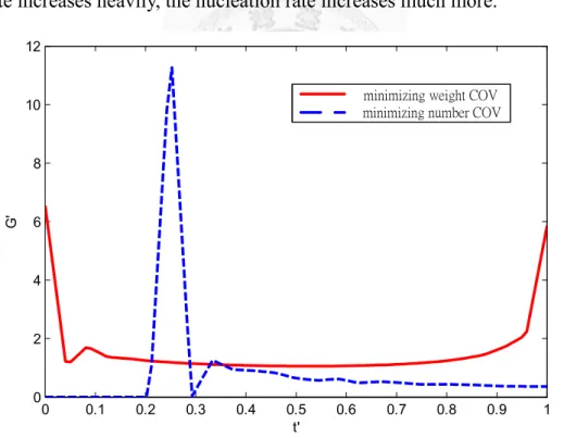
Both results from two objective functions show a narrow peak, however it is the nucleated crystals that give a narrow distribution. Figure 7 shows the optimal growth rate using objective function minimizing weight coefficient of variation and number coefficient of variation. When the supersaturation increases, both nucleation rate and growth rate will be enhanced. From Equation 13, we can see that the growth rate directly affect the nucleation rate.
Because of the power in Equation 13 γ is equal to three, when the growth rate increases heavily, the nucleation rate increases much more.
Figure 7: The optimal growth trajectory using objective function, minimizing
weight coefficient of variation and minimizing number coefficient of variation.
0 0.1 0.2 0.3 0.4 0.5 0.6 0.7 0.8 0.9 1
0 2 4 6 8 10 12
t'
G'
minimizing weight COV minimizing number COV
31
Figure 8: The optimal nucleation rate trajectory using objective function,
minimizing weight coefficient of variation and minimizing number coefficient of variation.
Figure 8 shows the nucleation rate trajectory. In this figure we can see that both of the objective functions result in large nucleation peak in the process. The objective function minimizing weight coefficient of variation causes excess nucleation at the beginning of the batch, and the objective function minimizing number coefficient of variation causes excess nucleation at the middle of the batch time. From Figures 6, 7 and 8 we can see that these two objective functions achieve narrow final crystal size distribution by making excess nucleation during the batch. Thus they achieve the minimum of
0 0.1 0.2 0.3 0.4 0.5 0.6 0.7 0.8 0.9 1
0 50 100 150 200 250
t'
B'
minimizing weight COV minimizing number COV
32
the objective function, however, the large amount of nucleated crystals and excess nucleation are not desirable.
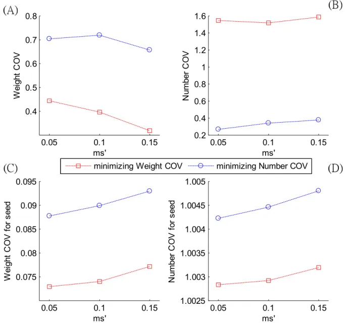
Figure 9: Weight coefficient of variation and number coefficient of variation
value for different objectives.
Figure 9 shows the resulting weight coefficient of variation and number coefficient of variation when both of these objectives are used as the objective
0.05 0.1 0.15
0.4 0.5 0.6 0.7 0.8
ms'
Weight COV
0.05 0.1 0.15
0.2 0.4 0.6 0.8 1 1.2 1.4 1.6
ms'
Number COV
minimizing Weight COV minimizing Number COV
0.05 0.1 0.15
0.075 0.08 0.085 0.09 0.095
ms'
Weight COV for seed
0.05 0.1 0.15
1.0025 1.003 1.0035 1.004 1.0045 1.005
ms'
Number COV for seed
33
function. As expected, in panel A, when the objective is to minimize the weight coefficient of variation, the weight coefficient of variation is indeed lower than the number coefficient of variation. In Panel B, again as expected, when the objective is to minimize the number COV, the number COV is indeed less than when the objective is to minimize the weight COV.
However, the situation if the nucleated crystals are filtered out (Panels C and D). In that case, minimizing the weight COV also minimizes the number COV, and using the number COV as the objective results in an inferior performance. Figure 7 shows the number distribution (f(l)) and the weight distribution (L3f(L)) of the product using the saturation concentration trajectory that minimizes the weight COV and the number COV. Minimizing the weight COV results in more growth of the seeds. On the basis of these two results, we conclude that among objectives that aim to minimize a COV, minimizing the weight COV is more suitable than minimizing the number COV.
34
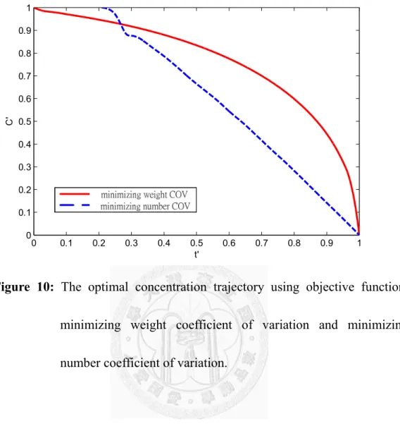
Figure 10: The optimal concentration trajectory using objective function,
minimizing weight coefficient of variation and minimizing number coefficient of variation.
0 0.1 0.2 0.3 0.4 0.5 0.6 0.7 0.8 0.9 1
0 0.1 0.2 0.3 0.4 0.5 0.6 0.7 0.8 0.9 1
t'
C'
35
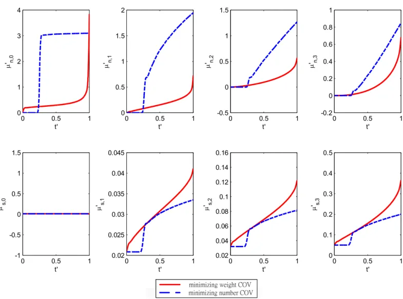
Figure 11: Different order of moment plot during the batch time for using
objective function minimizing weight coefficient of variation and minimizing number coefficient of variation.
0 0.5 1
0 1 2 3 4
t' µ' n,0
0 0.5 1
0 0.5 1 1.5 2
t' µ' n,1
0 0.5 1
-0.5 0 0.5 1 1.5
t' µ' n,2
0 0.5 1
-0.2 0 0.2 0.4 0.6 0.8 1
t' µ' n,3
0 0.5 1
-1 -0.5 0 0.5 1 1.5
t' µ' s,0
0 0.5 1
0.02 0.025 0.03 0.035 0.04 0.045
t' µ' s,1
0 0.5 1
0.02 0.04 0.06 0.08 0.1 0.12 0.14 0.16
t' µ' s,2
0 0.5 1
0 0.1 0.2 0.3 0.4 0.5
t' µ' s,3
36
4.4. Weight Mean Size and Number Mean Size
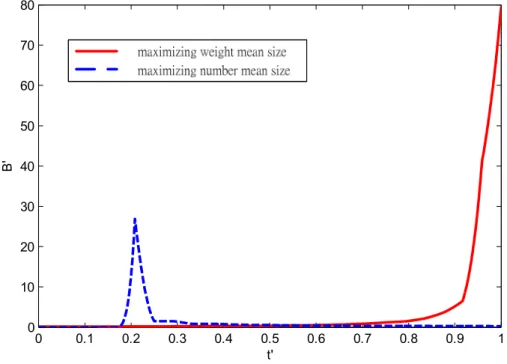
Figure 12 shows the optimal nucleation trajectory using object function minimizing weight mean size and minimizing number mean size. Again we can observer that for trajectory from result using objective function maximizing number mean size causes excess nucleation.
Figure 12: The optimal nucleation rate trajectory using objective function,
minimizing weight mean size and minimizing number mean size.
0 0.1 0.2 0.3 0.4 0.5 0.6 0.7 0.8 0.9 1
0 10 20 30 40 50 60 70 80
t'
B'
37
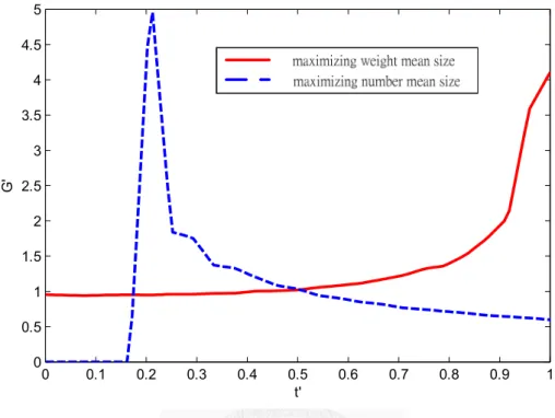
Figure 13: The optimal growth trajectory using objective function, minimizing
weight mean size and minimizing number mean size.
Figure 13 shows the optimal growth rate trajectory using objective function minimizing weight mean size and minimizing number mean size. We can observe that the batch is actually started when 't =0.16.
0 0.1 0.2 0.3 0.4 0.5 0.6 0.7 0.8 0.9 1
0 0.5 1 1.5 2 2.5 3 3.5 4 4.5 5
t'
G'
38
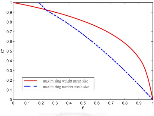
Figure 14: The optimal concentration trajectory using objective function,
minimizing weight mean size and minimizing number mean size.
Although the optimal trajectory of minimizing number mean size gives an excess early growth and shorten the batch time, it is still reasonable for objective function minimizing number mean size. In Figure 15 we can see that the excess nucleation from trajectory which is optimized using maximizing number mean size causes raising of zeroth moment at the early batch time.
However, at the end of the batch the zeroth moment from the optimal trajectory using maximizing weight means size is larger. Since the number mean size of the crystal is defined as µT,1/µ , the value of the zeroth T,0
moment is very important for number mean size when compare to the weight
0 0.1 0.2 0.3 0.4 0.5 0.6 0.7 0.8 0.9 1
0 0.1 0.2 0.3 0.4 0.5 0.6 0.7 0.8 0.9 1
t'
C'
39
mean size. And from Equation 26, the nucleation rate directly affects the value of the zeroth moment. Therefore, it is reasonable that the trajectory using maximizing number mean size as objective function by avoiding high growth rate when the third moment is larger at the end of the batch. And that is the major reason why the program chooses an early growth trajectory and shortens the batch time.
40
Figure 15: Different order of moment plot during the batch time for using
objectives function minimizing weight mean size and minimizing number mean size.
We compare objectives involving maximizing a mean size of the final product crystals, either the weight mean size or number mean size. Figure 16 shows the results for maximizing the weight mean size and the number mean size. In Panel A, as expected, if the objective is to maximize the weight mean
0 0.1 0.2 0.3 0.4 0.5 0.6 0.7 0.8 0.9 1
0 10 20 30 40 50 60 70 80
t'
B'
0 0.5 1
0 1 2 3 4
t' µ' n,0
0 0.5 1
0 0.2 0.4 0.6 0.8
t' µ' n,1
0 0.5 1
-0.2 0 0.2 0.4 0.6 0.8
t' µ' n,2
0 0.5 1
-0.1 0 0.1 0.2 0.3 0.4 0.5 0.6
t' µ' n,3
0 0.5 1
-1 -0.5 0 0.5 1 1.5
t' µ' s,0
0 0.5 1
0.06 0.07 0.08 0.09 0.1 0.11 0.12
t' µ' s,1
0 0.5 1
0.05 0.1 0.15 0.2 0.25 0.3 0.35 0.4
t' µ' s,2
0 0.5 1
0 0.2 0.4 0.6 0.8 1
t' µ' s,3
41
size, then the product crystals do indeed have a larger weight mean size than if the objective is to maximize the number mean size. Likewise, from Panel B, if the objective is to maximize the number mean size then the resulting product crystals do indeed have a larger number mean size than if the objective is to maximize the weight mean size.