國立臺灣大學工學院工業工程學研究所 碩士論文
Graduate Institute of Industrial Engineering College of Engineering
National Taiwan University Master Thesis
一般化縮減信賴域搜尋及其在多目標統計模型最佳化 之應用
Generalized Reduced Trust-region Search and Its Applications to Statistical Multi-Objective Optimization
陳彥廷
Yen-Ting Chen
指導教授:陳正剛 博士 Advisor: Argon Chen, Ph.D.
中華民國 97 年 8 月
August, 2008
謝誌
看著電腦中一個又一個的論文備份檔,與碩士學位論文及格證明,一次又一
次的Group Meeting,經歷了四個寒暑,無數個看日出的清晨,令人難忘的畢業
旅行,這其中最令人感到欣慰的一件事,莫過於論文的順利完成!在我的研究生 涯中,首要感謝的當然是我的指導教授陳正剛老師,老師對於學術研究的熱誠,
與對事物的嚴謹,與那融會貫通的教學方式,都是我一生當中值得學習的對象,
也要感謝老師在論文階段,對本論文內容做到滴水不露、逐字斧正的程度,實令 我深為感佩!另外,感謝口試委員的不吝指導,包括兩位從新竹不辭路途遙遠趕 來的柯志明與蔡雅蓉經理、與元智大學的范書愷老師,您的著作是本論文相當重 要的基石、所上的兩位老師,張時中老師與吳政鴻老師,承蒙五位口試委員在論 文口試上的指正與建議,使得本論文更加完備,在此也深表感激。感謝所辦最熱 心助理們,Monica、淑云、相怡,給與我許多生活與行政工作上的協助,與常常 提醒我要工讀的琍文,幫老師傳話的助理宇珊。感謝兩位學識淵博的博班學長,
Amos 在修課上的幫助與小藍在本論文的相關理論的討論與指導。也要感謝患難 與共的戰友們,回家與吃飯的好伙伴小耀、同為台南人全身名牌的靖淵、一起住 半年才了解他在想什麼的政緯、躺著也中槍但脾氣超好的建名、研究室守護者所 辦愛將凌誠、垂直正交化之神育維,講話無理頭的宅宅青杉、還有其他好同學們,
勝傑、于珈、哲欣、俊男、皙杰、俊儒、尚樺、建宏、韋銓,同為阿剛 Group
的學弟妹們,小薛薛、博尉、惟婷、士晉、信融。最後要感謝我最摯愛的家人們,
特別是無怨無悔對我的栽培與付出我的爸媽,常常關心我的爺爺與奶奶,相當支 持我的叔叔嬸嬸,還有大、小姑姑與大、小姑丈,還有一起長大的兄弟姐妹們,
沒有你們24 年來的支持也不會有今天的我。最後也要感謝這最後半年來,常常
聽我抱怨,但又為我鼓勵與打氣的采琳,願未來的路能與你共同努力。
論文摘要
一般化縮減梯度(Generalized Reduced Gradient)法是一個廣受喜愛的非線性 規 劃 問 題 解 法 , 但 於 具 有 四 次 目 標 式 之 多 目 標 統 計 最 佳 化(Statistical Multi-objective Optimization)問題中,一般化縮減梯度法容易出現搜尋路徑曲折 (Zigzagging)的現象。於本研究中,我們改善了信賴域(Trust Region)搜尋法,並 發展了一般化縮減信賴域(Generalized Reduced Trust Region)搜尋法。此方法結合 了一般化縮減梯度與信賴域搜尋法,將具有限制式的非線性規劃問題,轉化成由 非基礎變數(Nonbasic variable)所構成的不具現制式的非線性規劃問題,並且在縮 減空間(Reduced Space)中獲得最佳改善的方向,且於案例中克服了一般化縮減梯
度法的缺點,此外,我們也結合了一般化縮減信賴域搜尋法與Zoutendijk’s 搜尋
法以改善搜尋效果。最後,為了驗證該演算法的成效,我們利用一個眾所皆知且 具四次目標式的測試問題:Rosenbrock’s function 與三個案例來測試,第一個案 例是關於半導體可製造性設計(DFM)之問題,而第二個案例是半導體供應鏈穩健 配置之案例,最後一個案例為半導體製造過程中,臨界尺寸均勻度(CDU)在軌道 系統之曝光後烘烤(PEB)步驟下之最佳化。經由與商業套裝軟體 Lingo 的結果比 較,我們可以在相似的計算時間內獲得同樣甚至更好的最佳解。
關鍵字:非線性規劃,多目標統計最佳化,一般化縮減梯度法,一般化縮減信賴 域法,信賴域法
ABSTRACT
“Generalized Reduced Gradient” method is a popular NLP method, but it often incurs a zigzagging search path especially for the statistical multi-objective optimization (SMOO) problem where the objective function is a quartic function. In this study, we improve the “Trust Region (TR)” search method and develop the
“Generalized Reduced Trust Region” (GRT) search method which combines the GRG method and the improved TR method. The GRT search transforms the constrained NLP problem to an unconstrained NLP problem consisting of only the nonbasic variables and searches the best improving direction in the reduced space. The proposed method is shown to overcome the zigzagging problem of the GRG method. To verify the performance of our methods, we study a well know test problem and three cases. The test problem is called Rosenbrock’s function which has a quartic objective function with two decision variables. The first case is a semiconductor design for manufacturing (DFM) problem. The second case is the problem to configure a robust semiconductor supply chain. The final case is the “Track System PEB CDU Optimization”. Compared against the result of the commercial software “Lingo”, the same or better solutions are obtained by our methods with comparable computation time.
Keywords: Nonlinear Programming, Statistical Multi-Objective Optimization,
Generalized Reduced Gradient Method, Generalized Reduced Trust Region Method, Trust Region MethodTABLE OF CONTENTS
TABLE OF CONTENTS ... III LIST OF FIGURES ... V LIST OF TABLES ... VII
1 Introduction ... 1
1.1 Problem Definition and Formulation ... 1
1.2 Current NLP Methods Review ... 6
1.2.1 Generalized Reduced Gradient (GRG) Method ... 7
1.2.2 Ridge Analysis and Ridge Search Method ... 15
1.2.3 Zoutendijk Method... 20
1.3 Shortcomings of Current NLP Methods ... 23
1.3.1 Shortcomings of Generalized Reduced Gradient Method ... 23
1.3.2 Shortcomings of Ridge Search Method ... 28
1.4 Research Objectives ... 31
1.5 Thesis Organization ... 34
2 Trust Region Method ... 35
2.1 Trust Region Method ... 35
2.2 Iterative Solution of Trust Region Subproblem (TRS) ... 39
2.3 The Hard Case ... 43
2.4 Modifications of Trust Region Algorithm... 49
3 Generalized Reduced Trust Region (GRT) Search ... 63
3.1 Trust Region Search Method ... 63
3.2 Generalized Reduced Trust Region Method ... 71
3.3 Convergence Proof of Generalized Reduced Trust Region Method ... 94
4 Case Study ... 98
4.1 Geometric Layout Design for Semiconductor Manufacturability ... 98
4.2 Robust Configuration of Semiconductor Supply Chain ... 104
4.3 Track System PEB CDU Optimization ... 112
5 Conclusions ... 121
REFERENCE ... 124
Appendix A. Proof of the solution to the Hard Case ... 126
Appendix B. Trust Region Algorithm ... 127
Appendix C. Proof of Theorem 3.1 (Convergence to Stationary Point) ... 129
Appendix D. Problem Formulation of DFM Case ... 132
Appendix E. Expected Cycle Times and Raw Process Time of Supply Chain ... 133
Appendix F. Problem Formulation of Supply Chain Case ... 135
LIST OF FIGURES
F
IGURE
1.1RESPONSE SURFACE OF CHEMICAL PROCESS
... 3F
IGURE
1.2FEASIBLE
REGION OF
EXAMPLE
1.1WITH THE NONLINEAR CONSTRAINTS
.. 13F
IGURE
1.3FEASIBLE
REGION OF
EXAMPLE
1.1WITH THE LINEARIZED CONSTRAINTS
. 13 FIGURE
1.4THE
EXAMPLE
1.1IN REDUCED SPACE OF NONBASIC VARIABLES
... 14F
IGURE
1.5NEWTON
-RAPHSON METHOD IN THE ORIGINAL SPACE
... 14F
IGURE
1.6RIDGE PATH OF ALL STATIONARY POINTS WITH VARIOUS RADIUSES
... 16F
IGURE
1.7THE DEPENDENCE OF RADIUS ON
LAGRANGIAN MULTIPLIER
... 18F
IGURE
1.8THE DEPENDENCE RADIUS AGAINST
LAGRANGIAN MULTIPLIER
... 19F
IGURE
1.9ZOUTENDIJK
’S DIRECTION OF
EXAMPLE
1.1. ... 23F
IGURE
1.10QUADRATIC RESPONSE SURFACE
... 25F
IGURE
1.11QUARTIC RESPONSE SURFACE
... 25F
IGURE
1.12SURFACE PLOT AND CONTOUR MAP OF
EXAMPLE
1.3 ... 26F
IGURE
1.13SEARCH PATH OF
GRGIN
EXAMPLE
1.3 ... 27F
IGURE
1.14DASH
-LINE REGION IN
FIGURE
1.13 ... 27F
IGURE
1.15ZIGZAGGING PATH IN DASH
-LINE REGION OF
FIGURE
1.14 ... 28F
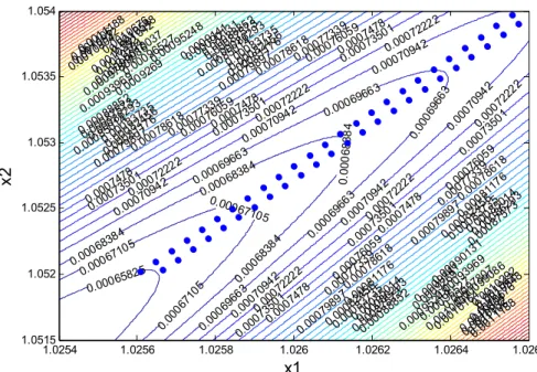
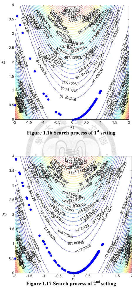
IGURE
1.16SEARCH PROCESS OF
1STSETTING
... 30F
IGURE
1.17SEARCH PROCESS OF
2NDSETTING
... 30F
IGURE
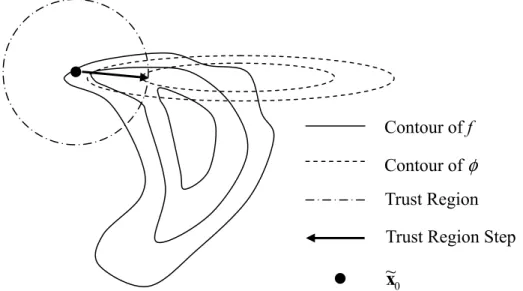
2.1TRUST
-REGION AND
TRUST
-REGION STEP
... 37F
IGURE
2.2THE RELATIONSHIP OF
1ΔAND
μIN EXAMPLE
1.2 ... 42F
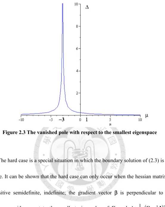
IGURE
2.3THE VANISHED POLE WITH RESPECT TO THE SMALLEST EIGENSPACE
... 46F
IGURE
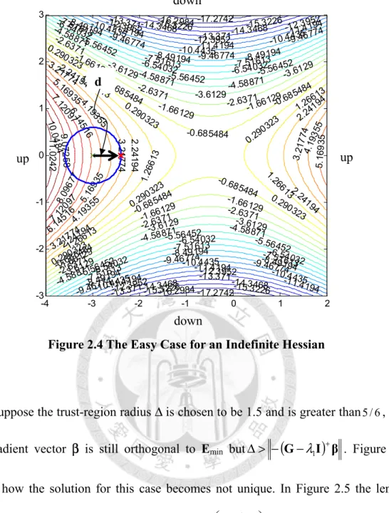
2.4THE
EASY
CASE FOR AN
INDEFINITE
HESSIAN
... 48F
IGURE
2.5THE
HARD
CASE FOR AN
INDEFINITE
HESSIAN
... 49F
IGURE
2.6THE FAILURE
NEWTON
’S ITERATION
... 54F
IGURE
2.7COMPARISON OF LOWER
-BOUND FOR
μIN SITUATION
1 ... 55F 2.8C - μ 2 ... 56
F
IGURE
2.9COMPARISON OF LOWER
-BOUND FOR
μIN SITUATION
3 ... 57F
IGURE
2.10μ
max,μ
min,μ
min( )
TAND μ
1ON TWO
-DIMENSIONAL SPACE
... 61F
IGURE
2.11SAFEGUARD MECHANISM FOR
NEWTON
’S ITERATE IN THE 1 Δ SPACE
... 62F
IGURE
3.1POSITIONS OF X
(1)AND X
(2)AT ITERATION
1WITH
Δ =( )1 0.5 ... 67F
IGURE
3.2THE INSIDE SOLUTION OF
ITERATION
2. ... 68F
IGURE
3.3THE REJECTED DIRECTION OF ITERATION
3.1 ... 69F
IGURE
3.4THE ACCEPTED DIRECTION OF ITERATION
3.2 ... 70F
IGURE
3.5THE SEARCH PROCESS OF
EXAMPLE
3.1 ... 71F
IGURE
3.6THE LINE SEARCH SOLUTION OF ITERATION
3 ... 72F
IGURE
3.7BOUNDARY SOLUTIONS BY PERFORMING LINE SEARCH
... 73F
IGURE
3.8THE INFEASIBLE DIRECTION GENERATED BY THE
TRMETHOD
... 74F
IGURE
3.9THE MAPPING OF THE SHRINKING FACTOR IN
(3.16) ... 82F
IGURE
3.10THE MAPPING OF THE ENLARGING FACTOR IN
(3.18) ... 83F
IGURE
3.11EXAMPLE OF
ZOUTENDIJK
’S METHOD
... 84F
IGURE
3.12THE IMPROVING DIRECTION IN THE REDUCED SPACE
... 88F
IGURE
3.13THE IMPROVING DIRECTION IN THE ORIGINAL SPACE
... 89F
IGURE
3.14THE SEARCH PROCESS OF THE
“GRT+ZOUTENDIJK
”METHOD
... 94F
IGURE
4.1TWO
SPICEMODELS WITH THE ROUNDING PHENOMENON
... 98F
IGURE
4.2DESIGN FACTORS ON GEOMETRIC LAYOUT
... 100F
IGURE
4.3SEMICONDUCTOR SUPPLY CHAIN
... 104F
IGURE
4.4SUPPLY CHAIN ALLOCATION DECISION VARIABLES
... 105F
IGURE
4.5SUPPLY CHAIN SIMULATION MODEL
... 106F
IGURE
4.6THE DISTRIBUTION OF MULTIZONE
PEBBAKE PLATE
... 113F 4.7T . ... 116
LIST OF TABLES
T
ABLE
1.1COMPARISON OF TWO DIFFERENT SETTINGS
... 29T
ABLE
3.1THE ALL ITERATIONS OF
EXAMPLE
3.1 ... 70T
ABLE
3.2THE METHODS COMPARED IN OUR RESEARCH
... 92T
ABLE
3.3THE INITIAL POINTS OF THE
ROSENBROCK
’S FUNCTION
... 92T
ABLE
3.4THE
RESULTS OF
ROSENBROCK
’S FUNCTION
(LOCAL
SEARCH
) ... 93T
ABLE
4.1UPPER BOUNDS AND LOWER BOUNDS FOR
3FACTORS
... 100T
ABLE
4.2DESIRED TARGETS AND SPECIFICATION WINDOWS FOR
DFM ... 102T
ABLE
4.3OPTIMUM DESIGN OF
DFMCASE
... 102T
ABLE
4.4RESPONSES GIVEN THE OPTIMUM DESIGN
... 102T
ABLE
4.5SENSITIVITY EFFECTS GIVEN THE OPTIMUM DESIGN
... 102T
ABLE
4.6RESULTS OF
DFMCASE
(LOCAL
SEARCH
) ... 103T
ABLE
4.7THE
ENVIRONMENT SETTING OF MODEL
... 106T
ABLE
4.8THE CAPACITY AT EACH FACILITY OF EACH TIER
... 106T
ABLE
4.9OPTIMUM DESIGN OF SUPPLY CHAIN CASE
... 111T
ABLE
4.10RESPONSES GIVEN THE OPTIMUM DESIGN
... 111T
ABLE
4.11RESULTS OF SUPPLY CHAIN CASE
(LOCAL
SEARCH
) ... 111T
ABLE
4.12SOURCE AND CHARACTERISTIC OF SEVERAL TYPES OF
CDVARIATION
... 113T
ABLE
4.13RESULTS OF
CDUOPTIMIZATION CASE
(LOCAL
SEARCH
) ... 1191 Introduction
1.1 Problem Definition and Formulation
Response surface methodology (RSM) is a powerful technique for quality and productivity improvement.
Many processes such as chemical processes, manufacturing processes, development processes, etc, are critical to productivity. These processes transform inputs into outputs. In chemical processes, reaction time and reaction temperature are inputs and the yield is output. Actually, engineers usually want to know how inputs affect outputs. Response Surface Methodology (RSM) is a set of mathematical and statistical techniques used by researchers and engineers to aid in the solution of certain types of problems. In RSM, we call the inputs and the outputs “explanatory (independent) variables” and “responses”. The response is normally measured on a continuous scale and is a measure representing the most important function of the system. The independent variables are the fade affecting the response and are usually controllable.
Suppose the yield of a chemical process is affected by two factors. The first one is reaction time and the second one is reaction temperature. At beginning we only
( )
+ε
=
f reaction tme reaction temperatur e
yeild
, . (1.1)In order to disinter the function f, engineers use RSM procedures involve experimental strategy, mathematical methods, and statistical inference which, when combined, enable them to make an efficient empirical exploration of the system in which they are interested. First, they design a set of designs using experimental strategy (design). The purpose of the experimental strategy (design) is to enable the analyst to explore the response surface [12] with equal precision, in any direction.
Subsequently engineers collect a set of data by performing these designs.
After obtaining these data, a model can be built by using regression analysis.
Here we suppose the linear multiple regression is applied. The relationship between response and factors is express as:
ε β
β
β
+ × + × +
= reaction time reaction temperatur e
yield
0 12
(1.2)
, where
β
1andβ
2mean the effects to yield by changing one unit reaction time and reaction temperature respectively. These two coefficients are useful information for analyzing the chemical process. It is also convenient to view the response surface in the two-dimensional time-temperature plane, as in Figure 1.1.
Figure 1.1 Response surface of chemical process
Normally, there are two stages of performing RSM. The first stage is called response surface design which is mentioned in last two paragraphs. The second stage is called response surface optimization or response surface analysis. In the latter stage, engineers use optimization techniques such as steepest descent/ascent method to decide the search direction for obtaining the best value of independent variable i.e.
reaction time and reaction temperature in our example.
In most engineering problem, the linear response surface model is not satisfactory. Indeed the relationship between response and predictor variable is nonlinear relationship. So we need nonlinear functions help us to describe the relationship well. Now we consider there are n predictor variables, and the i-th expected response is denoted as
yˆ
. The nonlinear response surface model can be0 10
20 30
40 50
-50 0
50 -400 -200 0 200 400 600 800
Yield
Reaction Time (second)
Reaction Temperature (
oC)
x B x x b
iT T ii
n n n n i i
i
n inn i
n in i
i i
n i
i
b
x x x
x x
x
x x
x b x
b x b b
x x f y
+ +
=
+ +
= +
+ + +
+ + + +
=
=
−
− 0
1 , 1 , 3
1 13 2 1 12
2 2
1 11 2
2 1 1 0
1
ˆ
ˆ ˆ
) (
ˆ
β β
β
β
)β
) LL L
L
(1.3)
, where
⎟⎟
⎟ ⎟
⎟
⎠
⎞
⎜⎜
⎜ ⎜
⎜
⎝
⎛
=
x
nx x M
2 1
x
denotes n variables;⎟⎟
⎟ ⎟
⎟
⎠
⎞
⎜⎜
⎜ ⎜
⎜
⎝
⎛
=
in i i
i
b b b M
2 1
b
, and
⎟⎟
⎟⎟
⎟
⎠
⎞
⎜⎜
⎜⎜
⎜
⎝
⎛
=
inn n i i
n i i
i
i
sym β
β β
β β
β
ˆ ˆ 2 ˆ
ˆ 2 ˆ 2
ˆ
2 22
1 11 12
M O L L
B
are the linear and quadratic coefficients, respectively.
Most engineering requirements would specify a desired target Ti for each response
yˆ
i. That is, the difference betweenyˆ
i and its target Ti should be as small as possible.Here, the quadratic loss function [1] can be used to measure the total difference. That is,
( )
0 22
( )
ˆ ∑
∑ − = + + −
i i i
T T i i i
i
w
iy
iT
iw b T
Min b x x B x
. (1.4)In (1.4), wi is a user-specified weight representing the relative importance for
yˆ
i to conform to the target. In this research, without loss of generality, all wi are assumed toequal to 1. In addition to the target, the response
yˆ
i should be located in a specification widow with an upper specification limit Ui and a lower specification limit Li:i i
T T i i
i
b U
L
≤ 0+b x
+x B x
≤ . (1.5)Moreover, each input variable xn usually has an experimental region with an upper bound
U and a lower bound
xnL :
xnn
n n x
x
x U
L
≤ ≤ .(1.6)
The purpose of the region is that if variable xn is out of the experimental region, the estimated response may be incorrect. So the regional constraints are needed. There are also some technical restrictions that can be expressed as linear equality constraints. In our example, we sometime request the linear combination of reaction time and reaction temperature hits the target Tp.
p p
p
T
a
0+a
Tx
= (1.7), where
⎟⎟
⎟⎟
⎟
⎠
⎞
⎜⎜
⎜⎜
⎜
⎝
⎛
=
pn p p
p
a a a
M2 1
a
are the linear coefficients for the p-th linear equality constraint.
Here we give a summary for our problem, let T represent the set of responses with targets; S represent the set of responses with specification windows; and Z represent the set of linear equality constraints. The optimization problem can be
formulated as:
T i T b
f Minimize
i i i
T T i
i
+ + − ∈
= ∑ (
0)
2)
( x b x x B x
x . (1.8)
n q
U x L
Z m p
T a
S m j
U b
L subject to
q
q q x
x
p p
p
j j
T T j j j
, , 1 .
, , 1
;
, , 1
; :
2 0
1 0
K K K
=
≤
≤
∈
=
= +
∈
=
≤ +
+
≤
x a
x B x x b
T
This is a nonlinear minimization problem subject to linear equality constraints, and nonlinear inequality constraints. In particular, the objective function is a quartic programming problem with the objective function being a “quadratic” of “quadratic”
and nonlinear inequality constraints being quadratic inequalities. Actually there are numerous non-linear programming (NLP) methods which can solve this problem, and these methods will be introduced in next section.
1.2 Current NLP Methods Review
For engineers, optimization is really a practical procedure. There are numerous NLP methods developed in recent half century. The most conventional class is
“Primal Method” also called “Methods of Feasible Direction” [2, 11]. The following strategy is typical feasible direction algorithm. Given a feasible point x, a feasible direction d is generated by main algorithm and the step size
λ
is also determined.Thus, these methods keep two properties (1)
x +
λd
feasible, and (2) the objective value of current iteration smaller than last iteration. These methods usually have thefollowing three advantages [2]:
1. Because these methods generate a feasible direction for minimizing the objective. Consequently the sequence of these points generated by these methods is feasible too.
2. If these methods generate a convergent sequence, the limit of the sequence will often satisfy the convergence prosperity, i.e., these methods are usually shown to converge to KKT solutions.
3. These methods are not limited to solve convex problem.
1.2.1 Generalized Reduced Gradient (GRG) Method
When dealing with linear constraint optimization, it is natural to add slack variables and use the linear equality constraints to eliminate some of the variables from the problem. Reduced Gradient method uses this idea and avoids the use of penalty parameter to search optimal solution. After that Generalized Reduced Gradient (GRG) method is developed for nonlinear constrained optimization problem.
Today GRG is already verified to be a precise and accurate method for solving NLP problems. There are many commercial optimization software packages like LINGO, Microsoft Excel, Lotus and MINOS are all developed base on GRG.
The reduced gradient method can be viewed as the logical extension of the gradient method to constrained optimization problems. We start with linearly constrained optimization problems and consider the following linear equality constraint problem.
0
: ) ( :
≥
=
x
b Ax
x to Subject
f Minimize
(1.9)
, where A is m × n matrix of rank m; b is m-vector.
There are some assumptions of this problem [2]:
1. f is continuously differentiable;
2. Every subset of m columns of the m × n matrix A is linearly independent;
3. Each extreme point of the feasible set has at least m positive components (non-degeneracy assumption).
Now let x be a feasible solution. The basic idea of reduced gradient method is dividing all variables into two sets, the set of basic variables xB and nonbasic variables
x
N.For simplicity of notation we assume that we can partition the matrix A as A = [B,N] where B is an m × n
invertible matrix. We partition x accordingly:[
B N]
TT
x x
x
= , . Thus we can rewrite Ax = b as the follows.Bx
B + NxN = b , wherex
B = B−1b
− Β−1Nx
N. (1.10)0
0 )
( :
1 - 1 -
≥
≥
−
N
N N
N
: Subject to
f Minimize
x
Nx B b B
x
. (1.11)
, where fN (xN) = f (B−1
b
− Β−1Nx
N, xN).In (1.11), the variables we concerned are reduced to xN. If we have xN, we can obtain
x
B by substituting xN into (1.10). Now let’s consider the choice of search direction.Suppose d is a feasible direction, by the definition d should satisfy the condition
0
) ( <
∇ f x
Td
. And then we also translate the condition into (1.9) by dividing∇ f (x )
and d into two sets.0 )
( )
( B N N
B +∇ <
∇
f x
Td f x
Td
(1.12),where ∇B
f
(x
)is the gradient with respect to the basic variables.If d is a feasible direction, and then d satisfies the condition Ad=0, i.e. BdB + NdN = 0.
This means dB = −B−1
Nd
N. (1.13)And then substitute (1.13) into (1.12) to yield:
0 )
( )
( )
( =−∇ 1 +∇ <
∇ − T N
N T
B
f
f
f x d x B N x d
(1.14)In (1.14), we call
r
=−∇f
B(x
)TB
−1N
+∇f
N(x
)Td
N the reduced gradient of f at x for the given basis B. In other words, the reduced gradient r plays the same role in the reduced problem as the gradient f∇ did in the original problem. In fact, the reduced gradient is exactly the gradient of the function fN with respect to xN in the reducednonlinearly constrained optimization problems by linearizing the nonlinear constraints.
So we can solve the problem similarly to the linearly constrained case. The nonlinearly constrained problem with bounded constraints is express as follows.
n j
for U
x L
m i
for g
to subject
E for
f Minimize
j j j
i
n
, ,
~ 1
, ,
~ 1 0
) (
) (
~
~
~
~
K K
=
≤
≤
=
≤
∈ x
x
x
x
(1.15)
Given a nondegeneracy assumption, i.e., any columns of ∇
h ( ) x
given by linearization inequality constraints are linear independent, a summary of Generalized Reduced Gradient method is given as follows [2]:y Step 1:
Add slack variables to inequality constraints
g
~i( x ) ≤ 0
and obtain equalityconstraints
h
i~( ) x
=0,~i
=1,K,m
. Let x(k) be a feasible solution at the k-th search step.Linearize the constraints and get
∇ h ( x
(k))( x − x
(k)) = 0
. Decompose variables into basic and nonbasic sets (x
(Bk),x ). Furthermore, the Jacobian matrix
(Nk)∇ h ( x
(k))
is decomposed into∇ h ( x
(Bk))
and∇h
(x
(Nk)), such that∇ h ( x
(Bk))
is invertible.y Step 2:
Let
r
T =∇Nf
(x
(k))T −∇Bf
(x
(k))T∇Bh
(x
(k))−1∇Nh
(x
(k)) . Compute the vector dNwhose
~ j
th componentd
~j is⎪⎩
⎪⎨
⎧
−
<
=
>
= =
otherwise
0 and or
, 0 and if
0
~
~ ) ~
(~
~ ) ~
(~
~
j
j j k j j
j k j
j
r
r U x r
L
d x
(1.16), where
r
~j is the~ j
th component ofr.
If dN = 0, stop. x(k) is a KKT point; otherwise, go to step 3.
y Step 3.1:
Find a solution to satisfy the nonlinear constraints by Newton-Raphson method.
Choose
ε
> 0 and a positive integerT . Letθ
> 0 be such thatL
N ≤~x
N(k) ≤U
N, where~x
N(k) =x
(Nk)+θ d
N. Lety
(1)= x
(Bk) and t = 1.y Step 3.2:
Compute
y
(t+1)=y
(t)−∇Bh
(y
(t),~x
N(k))−1h
(y
(t),~x
N(k)) . IfL
B≤ y
(t+1)≤ U
B ,f
(y
(t+1),~x
N(k)) ), ( (Bk) (Nk)
f x x
< , and
(
+, ~
(N)) <
ε) 1 (t
x
ky
h
, letx
(k+1) =(y
(t+1),~x
N(k)) and go to step 1;otherwise, go to step 3.3.
y Step 3.3:
If t =T , replace θ byθ
/ 2
. Let ~x
N(k) =x
(Nk)+θ d
N andy
(1)= x
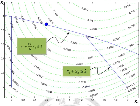
(Bk). Replace t by 1 and repeat step 3.2. Otherwise, replace t by t + 1 and repeat step 3.2.The contour in original space of the NLP problem is shown in Figure 1.2. In step 1, all inequality constraints are transformed into linearized equality constraints as shown in Figure 1.3. The selected basic variables are x1 and x2 and the selected nonbasic variables are x3 and x4. In step 2, the original NLP problem is transformed into a NLP problem without equality constraints in the reduced space of nonbasic variables, x3 and x4. The improving direction of the nonbasic variables is the opposite direction of the reduced gradient. However, the variables should not be negative. The improving direction of the nonbasic variables is modified as shown in Figure 1.4. In step 3, the improving direction after transformed into the original space is actually the direction along the tangent of the binding constraint. The optimal solution is then found through Newton-Raphson method as shown in Figure 1.5.
Example 1.1:
(
1,
2) 2
122
222
1 24
16
2: f x x x x x x x x
Minimize = + − − −
x ,
. 0 ,
; 8 . 6 2
17
; 2 :
2 1
2 2 1
2 1
≥
≤ +
≤ +
x x
x x
x
x
to
subject
Figure 1.2 Feasible Region of Example 1.1 with the nonlinear constraints
Figure 1.3 Feasible Region of Example 1.1 with the linearized constraints
-8.8074 -8.8074
-8.178
-8.178 -7.5486
-7.5486 -6.9192
-6.9192
-6.9192 -6.28
98
-6.2898 -6.2898
-5.66 04
-5.6604 -5.6604
-5.031
-5.031
-5.031
-5.031 -4.40
16
-4.4016
-4.4016
-4.4016 -3.77
23
-3.7723
-3.7723
-3.7723 -3.14
29
-3.14 29
-3.1429
-3.1429 -2.5
135
-2.5135
-2.5135
-2.5135 -1.88
41
-1.8841
-1.8841
-1.8841 -1.254
7
-1.2547 -1.2547
-1.2547 -0.62528
-0.62528 0.0041
123 0.0041123
0.63351
?
0 0.2 0.4 0.6 0.8 1 1.2 1.4 1.6 1.8 2
0 0.2 0.4 0.6 0.8 1
X
2X
1-8.8074 -8.8074
-8.178 -8.178
-7.5486
-7.5486 -6.91
92
-6.9192
-6.9192 -6.2
898
-6.2898 -6.2898
-5.66 04
-5.6604
-5.6604 -5.031
-5.031
-5.031
-5.031 -4.40
16
-4.40 16
-4.4016 -4.4016
-3.77 23
-3.77 23
-3.7723 -3.7723
-3.14 29
-3.1429
-3.1429
-3.1429 -2.5
135
-2.51 35
-2.5135
-2.5135 -1.884
1
-1.8841
-1.8841
-1.8841 -1.25
47
-1.2547
-1.2547-1. 25 47
-0.62528
-0.62 528
0.004
1123 0.0041123
0.6 33 51
?
0 0.2 0.4 0.6 0.8 1 1.2 1.4 1.6 1.8 2
0 0.2 0.4 0.6 0.8 1
5 5 2 4
1+
x
+x
=x
3
2
2
1
+
x+
x=
x 6 5
17
2
1+ x ≤
x
2 2
1 + x ≤
x
x
1x
2Figure
Fi
-4.40 -3 16
.77 23
-3.14 29
-2.5 135 -1.88 41 -1.254
7
-0.6252 0.0041
123 0 0 0.2 0.4 0.6 0.8 1
X
21.4 The Ex
igure 1.5 N
-5.66 04 -5.031 440
16
-4.
-3.7723
-3.14 -2
528 23
0.2 0.4
Redu
5 2
1+ x +
x
xample 1.1
Newton-Rap
-7.5486 -6.9192 -6.28
98
-5.031 4.4016 3
429 2.5135
-1.8841 -1.2547
?
0.6 0.8
d
Nuced Grad
d
4 =5 + x
in reduced
phson meth
-6.2898 -5.6604
-4.4 -3.7723
-3.14 -
8 1
ient
N d
2
1
+ x +
x
d space of n
hod in the o
-8.8074
-8.178 -7.5486 -6.9192
-5.031
4016
429
-2.5135 -1.8841
-1.2547 -0.62528
1.2 1.4
Optima Newton-Ra
3
= 2 + x
nonbasic va
original spa
-6.2898 -5.6604
-4.4
-3.7723 -3.14
-2
1.6 1.8
al Solution aphson M
ariables
ace
-8.8074 -8.178
-6.9192
-5.031
4016
429 2.5135
-1.8841 -1.2547
0.0041123 0.63351
2
X
1n
ethod
1.2.2 Ridge Analysis and Ridge Search Method
In RSM, ridge analysis is a method for exploring optimal factor levels of a response surface. Ridge analysis helps us to find maximum or minimum a quadratic response surface under a spheral constraint. The purpose of spheral constraint is to fixed distances from the center of the experimental region. Due to the formulation ridge analysis, it is a nonlinearly constrained optimization problem.
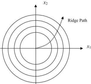
The concept of ridge analysis is finding an absolute minimum or maximum on the spheral constraint of a certain radius you trusted. Additionally, we can adjust the radius to increase the sphere size if the point on the spheral constraint is still inside the experimental region. In other words we can find an optimum corresponding to a distinct radius, all optimums with various radiuses construct a “ridge path” as shown in Figure 1.6. In fact, control radius of the region is hard in ridge analysis. We discuss the issue in the following subsection.
Figure 1.6 Ridge path of all stationary points with various radiuses
Consider the following problem.
2 0
2 ˆ 1
) (
Δ
=
+ +
=
subject to
b y Maximize Minimize
T
T T
x x
Gx x x β
(1.17)
, where x is an n-vector; G is the matrix contains quadratic coefficients; β is a vector expressed first order coefficients.
Under the problem formulation, global constrained optima are typically obtained using the Lagrangian multiplier approach. By introducing the Lagrangian multiplier
μ
, the problem will be an unconstrained optimization problem.) ˆ (
)
( Maximize L = y + x
Tx − Δ
2Minimize
μ (1.18)Differentiate (1.18) with respect to x, and then set the derivative equal to zero. The equation which includes a stationary point
xˆ
s will hold:ˆ 0 )
( + =
+ G I x
sβ
μ (1.19)x
1x
2Ridge Path
Given a fixed value of
μ
, the stationary pointxˆ
s on the sphere with radius Δ can be estimated to be:β I G
x
ˆs =−( +μ
)−1 (1.20)Theoretically, there are totaling n+1 equation, namely, the spherical constraint in (1.17) and (1.18) let us solve
xˆ
sandμ
. Practically the radius Δ is also unknown, i.e.there are n+2 unknown variables. That is we can’t solve
xˆ
sdirectly. So ridge analysisconsiders the following strategy to solve the problem.
1. Regard Δ as variable, but fix
μ
instead.2. Choose
μ
as a fixed value and substituteμ
with the fixed value into (1.19) to obtainxˆ
s.3. Evaluate y) by (1.17)
Even if we have the above strategies, there is still a problem that is how to choose
μ
. Providentially, there are some properties of ridge analysis help us chooseμ
appropriately. These properties are described as follows [7]:
1. At
μ = −∞ or ∞
then Δ = 0 and Δ increases exponentially to infinity at μ =λ
i.2. If we wish to find the ridge path as Δ varies, we can substitute any value of
μ larger than
− .λ
1The value μ determines the radius Δ, i.e., Δ is a function of
μ
. Figure 1.7 shows the relation between radius and Lagrangian multiplier.λ
1,…,λ
k are the eigenvalues of theG, and λ
k >λ
k-1 > … >λ
1.Figure 1.7 The dependence of radius on Lagrangian multiplier
We consider the following example to show you the relationship between Δ and
μ
.Example 1.2:
Δ
= +
=
2 2 2 1
2 2 2 1 2 1 2
1
2
2 1 2 2 1
15 x x to subject
x + x x + x + +x x + Minimize y
Express in matrix notation.
[ ]
[ ] ⎥ = Δ
⎦
⎢ ⎤
⎣
⎡
⎥ ⎦
⎢ ⎤
⎣
⎥ ⎡
⎦
⎢ ⎤
⎣
= ⎡
2 1 2 1
2 1 2 1 2
1
:
2 15 1
:
x x x x to subject
x x x x x +
+ x y
Minimize β
TG
Locus of absolute minima
1 μ
λ
−
−1
−
λ
k− λ
2λ
k−
Δ
, where ⎥
⎦
⎢ ⎤
⎣
=⎡ 1
β
2 ; ⎥⎦
⎢ ⎤
⎣
=⎡ 1 2
2
G
1 ; the eigenvalues of G are −1 and 3; the correspondingeivenvectors
[ ]
−1 ,1T and[ ]
1 ,1T.Introduce Lagrangian multiplier
μ
and then we have( )
⎥ ⎥
⎥ ⎥
⎦
⎤
⎢ ⎢
⎢ ⎢
⎣
⎡
+ +
− +
− −
+ +
−
−
⎥ =
⎦
⎢ ⎤
⎣
⎥ ⎡
⎦
⎢ ⎤
⎣
⎡
+
− +
= +
−
=
−
−
2 1 2
1
2 3
3 2 3
2 1
2 1
2
2
~ 1
μ μ μ μ μ μ μ
μ I β μ G
x
s (1.21)We also have
2 2
2
2 2
2 2
) + 2 3 (
5 + 6 9
2 3
3 2 3
2
2 3
3 2 3
2
~
~
μ
μ μ
μ
μ μμμ μμ μ
μμμ μμ
+
−
= −
⎥ ⎥
⎥ ⎥
⎦
⎤
⎢ ⎢
⎢ ⎢
⎣
⎡
+ +
− +
− −
+ +
−
−
⎥ ⎥
⎥ ⎥
⎦
⎤
⎢ ⎢
⎢ ⎢
⎣
⎡
+ +
− +
− −
+ +
−
−
=
= Δ
T s
T s
x x
(1.22)
That is Δ is a function of
μ
, figure 1.8 shows the relationship on a two dimension space.−λ1 Δ
μ
In (1.22), the denominator in the radical has two factors. We can factorize the denominator as:
( 3 )( 1 )
+ 2
3 +
2= + −
−
μ μ μ μ (1.23)(1.22) also implies that if
μ
is equal to the subtractive eigenvalue of G, i.e. −3 or 1, the denominator is close to 0. Therefore Δ goes to positive infinity. On the other hand, ifμ
goes to positive or negative infinity, thus the denominator is close to positive zero, i.e., Δ goes to zero.1.2.3 Zoutendijk Method
Zoutendijk’s method searches a feasible improving direction. Compared with the GRG method, the direction may be less effective. To consider (1.15) (a minimization problem), if the direction is an opposite direction to objective function’s gradient, it is an improving direction. Moreover, if the direction is an opposite direction to binding constraint’s gradient, it is a feasible direction. Zoutendijk’s method solves a linear program to generate a direction satisfying the above two requirements; to improve and to be feasible.
Zoutendijk’s method is described as follows:
y Step 1:
Let
x
(k) be a feasible solution at the k-th search step. Check the binding nonlinear constraints. Let W~= {
w ~
:g
w~(x
( )k )=0 }. Compute the gradients of the objective function and the binding constraints∇ f ( x
( )k)
and ~( ( )k )g
wx
∇ with respect to
x
(k).y Step 2:
Solve the following linear program with decision variables dZ
and z:
z Minimize
z
:
,d .
. ...
1 1 1
~; 0 ~
) (
; 0 )
( :
Z )
~ (
Z ) (
n j d
W w z
g
z f
to subject
j T k w
T k
=
≤
≤
−
∈
∀
≤
−
∇
≤
−
∇
d x
d x
Let (z*
, d
Z*) be the optimal solution. If z* = 0, stop; x(k) is an optimal point. Else, go to the step 3.y Step 3:
Do Line Search along dZ*. Let the feasible solution be x(k+1). Return to step 1.
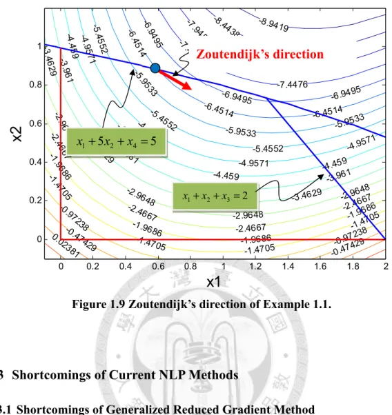
Here we also use the example 1.1 to introduce Zoutendijk’s method. Suppose that we start from iteration with current solution (x1, x2) = (0.5889, 0.8833) is also
binding on the second constraint in example 1.1. The gradients of objective function and constraint are described as follows:
( 3.4110 , 3.6442 )
) ,
(
1 2 T= − −
∇ f x x
, and( )
1,5) , ( 1 2 T
) 11 . 1
( =
∇
g x x
.Now we consider the following linear programming problem:
z Minimize
z
:
,d .
( )
( )
. 1 1
; 1 1
; 0 5
, 1
; 0 3.6442
, 3.4110 :
2 1 2 1
2 1
≤
≤
−
≤
≤
−
≤
⎟⎟ −
⎠
⎜⎜ ⎞
⎝
⎛
≤
⎟⎟ −
⎠
⎜⎜ ⎞
⎝
− ⎛
−
d d d z d
d z to d
subject
By performing simplex method, we can obtain the improving direction d is (d1, d2) = (1, −0.5102). We sketch the direction in Figure 1.9. We can see that the next solution can leave the binding constraint by performing line search along Zoutendijk’s direction. This will help us develop the main search algorithm of this thesis. It is detailed in chapter 3.
Figure 1.9 Zoutendijk’s direction of Example 1.1.
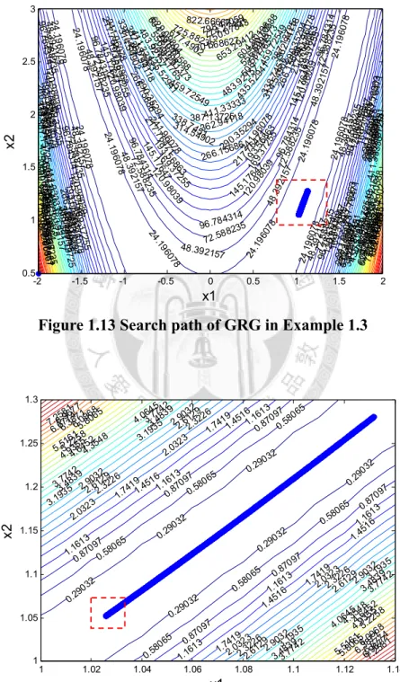
1.3 Shortcomings of Current NLP Methods
1.3.1 Shortcomings of Generalized Reduced Gradient Method
One motivation of this study is to overcome some unexpected phenomenon rose by the GRG method, although the GRG method is applied intensively in practice. The phenomenon is called “zigzagging” or “jamming”. Zigzagging usually appears at the later phase of search and causes a poor convergence. As mentioned earlier, the GRG method employs the first-order approximation:
f ( x
(k)+
λd ) = f ( x
(k)) +
λ∇ f ( x
(k))
Td
+ , where d is the search direction, e is the error of the linearization approximation.
e
When x(k) is close to the stationary point,∇ f x (
(k))
becomes very small so is the term-8.9419 -8.4438
-8.4438 -7.9457
-7.9457 -7.4476
-7.4476 -6.9
495
-6.9495 -6.9495
-6.451 4
-6.4514 -6.4514
-5.95 33
-5.9533 -5.9533
-5.45 52
-5.4552
-5.4552 -4.95
71
-4.9571
-4.9571
-4.9571 -4.459
-4.459
-4.459 -4.459
-3.961
-3.961
-3.961 -3.961
-3.46 29
-3.4629
-3.4629 -3.4629
-2.9 648
-2.9648
-2.9648
-2.9648 -2.46
67
-2.4667
-2.4667
-2.4667 -1.96
86
-1.9686
-1.9686
-1.9686 -1.47
05
-1.4705 -1.4705
-1.4705 -0.97238
-0.97238 -0.47429
-0.47429 0.02381
x1
x2
0 0.2 0.4 0.6 0.8 1 1.2 1.4 1.6 1.8 2
0 0.2 0.4 0.6 0.8
1
Zoutendijk’s direction
5 5 2 4
1+
x
+x
=x
3
2
2
1