B介子至η介子和h介子之二體稀有衰變與電荷宇稱對稱破壞之量測

(1)

國立臺灣大學理學院物理研究所碩士論文

Department of Physics Collage of Science

National Taiwan University Master Thesis

B 介子至η介子和 h 介子之二體稀有衰變與電荷宇稱對稱破壞之量測

Measurements of Branching fractions and CP Asymmetries of B→ηh decays

許祖達 Chou Tat Hoi

指導教授：張寶隸 Advisor: Paoti Chang

中華民國 100 年 8 月

(2)

Acknowledgment

First I would like to thank my parents for their supports that allow me to finish the educations. Also, I am grateful to everyone who gives me comments and suggestion. Especially, I thank my advisor Paoti Chang, people work or study in Belle Collaboration, and

members in NTUHEP.

(3)

中文摘要

在此篇論文中,我們使用了日本國家高能加速器中心 B 介子工廠 (KEKB) 及其 Belle 偵測器。我們從 772×10

⁶

B 介子對中分析了 B 介子至 η 介子和 h 介子之二體稀有衰變與電荷宇稱對稱破壞。其中 η 介子由兩個光子或三個π介子重組而成。h 介子則分別代表了帶電 K 介子，電π介子和中性 K 介子。

最後我們在和衰變中找到超過 3σ的電荷宇稱對稱破壞徵兆。同時我們也首次量測到衰變。

K

B^  ^ B^  ^

0 0

K B  

(4)

Abstract

We present the improved measurements of the B → ηh branching fraction and CP asymmetries using a data sample of 711 fb⁻¹ that contains 771.58± 10.57 million BB pairs collected on Υ(4S) resonance with the Belle detector at the KEKB asymmetric energy e⁺e⁻ collider. Here h means π^±, K^± and K_S⁰. And η is selected in η → γγ and η → π⁺π⁻π⁰ decays.

The evidence of CP asymmetry for B^± → ηK^± is found with 3.8 σ, and 3.0 σ in B^± → ηπ^± CP asymmetry. The branching fraction of B⁰ → ηK⁰ is observed with 5.4 σ standard deviation from zero.

(5)

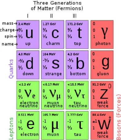
List of Figures

1.1 The three generation quarks and leptons, with the gauge bosons in the rightmost column. . . 2 1.2 Examples of Feynman diagrams involved in B^± → ηK^± decay. 5 1.3 Examples of Feynman diagrams involved in B^± → ηπ^± decay. 6 1.4 Examples of Feynman diagrams involved in B^± → ηKS⁰ decay. 6

2.1 Schematic layout of KEKB from the top and side view. . . 10 2.2 The structure of the Belle detector in isometric and side view. [26]. 11 2.3 The cross-section of the beam pipe at the IP [25]. . . 13 2.4 The structure of the beam pipe and horizontal masks [25]. . . 13 2.5 Conﬁguration of SVD [25]. . . 14 2.6 Side view of forward EFC (left) and isometric view of the

forward and backward EFC detectors (right) [25]. . . 15 2.7 Overview of CDC structure [25]. The lengths in the ﬁgure are

in units of mm. . . 16 2.8 Cell structure (left) and the cathode sector conﬁguration (right) [25].

18

(10)

2.9 The plot of dE/dx and particle momentum, together with the expected truncated mean [25]. . . 19 2.10 The arrangement of ACC in the Belle detector [25]. . . 20 2.11 Schematic drawing of a typical ACC counter module: (a) bar-

rel and (b) end-cap ACC [25]. . . 20 2.12 A TOF/TSC module [25]. . . 21 2.13 Mass distribution from TOF for particle momenta below 1.2

GeV/c [25]. . . . 22 2.14 The CDC, ACC and TOF are useful for particle identiﬁcation

in diﬀerent momentum region [26]. . . 23 2.15 Conﬁguration of ECL [25]. . . 23 2.16 Cross-section of a KLM superlayer [25]. . . 24 2.17 Pass rate of the muon preselection (primary requirement is

two associated KLM hits at least) for muons (open circle) and pions (closed circle) within 23^◦ < θ < 150 ^◦. The crosse are for muons with one hits at least [27]. . . 24

3.1 The Siganl MC ∆E and M_bc distribution and P.D.F.S. . . 32

4.1 The momentum topology of jet-like qq events and spherical- like BB events. . . . 33 4.2 The distributions of M_miss and Fisher discriminant for each

M_miss bin. The left ﬁgures stands for η(γγ)K^± and right ones stands for η(π⁺π⁻π⁰)K^±. The red line stands for signal MC and blue line stands for qq MC. . . . 36

(11)

4.3 The distributions of the components ofLR and itself. The top three figures denote Fisher discriminant, cosθ_B, and ∆Z for the B^± → η(γγ)K^± decay while the middle three ones are for B^± → η(π⁺π⁻π⁰)K^± decay. The bottom left figure denotes the LR distribution for B^± → η(γγ)K^± decay, and the The bottom right figure is for B^± → η(π⁺π⁻π⁰)K^± decay. The blue line stands for signal MC while the red line stands for qq

MC. . . 37

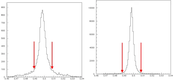
4.4 The ”q_B× q × r” distributions for B^± → ηK^± (lef t) and ”r” distributions for B^±→ ηK_S⁰(right). . . . 38

4.5 ∆E and M_bc ﬁtting result in 2D ensemble test . . . 40

4.6 ∆E M_bc, and LR ﬁtting result in 3D ensemble test . . . . 41

4.7 Pull, yield, error in 2D ensemble test . . . 42

4.8 Pull, yield, error in 3D ensemble test . . . 43

4.9 The generic BB background ∆E− Mbc scatter plots. . . 46

4.10 The rare BB background ∆E− Mbc scatter plots. Signal and feedacross background are already removed. . . 47

4.11 The rare BB background ∆E− Mbc scatter plots. Signal and feedacross background are already removed. . . 48

4.12 The signal (red) and feed across background (blue) ∆E and M_bc distribution and relative ratio in B→ ηh decay. . . 49

5.1 The ∆E (left) and M_bc(right) distribution for B⁺ → D⁰(K⁺π⁻π⁰)π⁺ signal MC. . . 52

5.2 The translated LR distribution for B⁺ → D⁰(K⁺π⁻π⁰)π⁺ signal MC. . . 52

(12)

5.3 The ∆E (left) and Mbc(right) distribution for B⁺ → D⁰(K⁺π⁻π⁰)π⁺ realdata (Exp. 7 : 65). . . 53 5.4 The translated LR distribution for B⁺ → D⁰(K⁺π⁻π⁰)π⁺

realdata (Exp. 7 : 65). . . 53 5.5 The D⁰ mass distribution of inclusive D⁰ → K⁺π⁻π⁰ decay,

in cc MC (top) and real data (down). . . . 54

6.1 The 3D ﬁt ∆E, M_bc and translated LR plots in ηh siganl MC (from left to right). . . 60 6.2 The 3D ﬁt ∆E, M_bc and translated LR plots in ηh siganl MC

(from left to right). . . 61 6.3 The projection plots from ensemble test. The red line is signal

PDF, blue line is continuum background, green for rare B and yellow for freedacross. The ∆E plot is showed with projection M_bc > 5.27 andLR > 0.7. Mbc plot is showed with projection

−0.15 < ∆E < 0.1 and LR > 0.7. LR plot is showed with projection −0.15 < ∆E < 0.1 and Mbc > 5.27. The top one is from B^± → η(γγ)K^± mode, and the bottom one is from B^± → η(γγ)π^±. . . 63 6.4 The ensemble test result in B^± → η(γγ)K^±mode. Pull(upper

left side), yield(upper right side) and error(bottom) distribution. . . 64 6.5 The ensemble test result in B^± → η(γγ)π^± mode. Pull(upper

left side), yield(upper right side) and error(bottom) distribution. . . 65

(13)

6.6 The projection plots from ensemble test. The ∆E plot is showed with projection M_bc > 5.27 and LR > 0.7. Mbc plot is showed with projection −0.1 < ∆E < 0.08 and LR > 0.7.

LR plot is showed with projection −0.1 < ∆E < 0.08 and M_bc > 5.27. The top one is from B^± → η(π⁺π⁻π⁰)K^± mode, and the bottom one is from B^± → η(π⁺π⁻π⁰)π^±. . . 66 6.7 The ensemble test result in B^± → η(π⁺π⁻π⁰)K^±mode. Pull(upper

left side), yield(upper right side) and error(bottom) distribution. . . 67 6.8 The ensemble test result in B^± → η(π⁺π⁻π⁰)π^±mode. Pull(upper

left side), yield(upper right side) and error(bottom) distribution. . . 68 6.9 The projection plots from ensemble test in B^± → η(γγ)KS⁰

mode. The ∆E plot is showed with projection M_bc > 5.27 and LR > 0.7. Mbc plot is showed with projection −0.15 <

∆E < 0.1 and LR > 0.7. LR plot is showed with projection

−0.15 < ∆E < 0.1 and Mbc> 5.27. . . . 69 6.10 The ensemble test result in B⁰ → η(γγ)K_S⁰ mode. Pull(upper

left side), yield(upper right side) and error(bottom) distribution. . . 70 6.11 The projection plots from ensemble test in B⁰ → η(π⁺π⁻π⁰)K_S⁰

mode. The ∆E plot is showed with projection Mbc > 5.27 and LR > 0.7. Mbc plot is showed with projection −0.15 <

∆E < 0.1 and LR > 0.7. LR plot is showed with projection

−0.15 < ∆E < 0.1 and Mbc> 5.27. . . . 71 6.12 The ensemble test result in B⁰ → η(π⁺π⁻π⁰)K_S⁰ mode. Pull(upper

left side), yield(upper right side) and error(bottom) distribution. . . 72

(14)

6.13 The ﬁt bias of signal and background in B^± → η(γγ)K^± and B^± → η(γγ)π^± mode. Only small bias in signal and rare B background in B^± → η(γγ)K^± mode. . . 73 6.14 The ensemble test result in B^± → η(γγ)K^±mode. Pull(upper

left side), A_CP(upper right side) and error(bottom) distribution. The PDG value is equal to -0.37. . . 74 6.15 The ensemble test result in B^± → η(γγ)π^± mode. Pull(upper

left side), ACP(upper right side) and error(bottom) distribution.The PDG value is equal to -0.13. . . 75 6.16 The ensemble test result in B^± → η(π⁺π⁻π⁰)K^±mode. Pull(upper

left side), A_CP(upper right side) and error(bottom) distribution. The PDG value is equal to -0.37. . . 76 6.17 The ensemble test result in B^± → η(π⁺π⁻π⁰)π^±mode. Pull(upper

left side), A_CP(upper right side) and error(bottom) distribution.The PDG value is equal to -0.13. . . 77 6.18 The ensemble test result in B⁰ → η(γγ)KS⁰ and B⁰ → η(π⁺π⁻π⁰))K_S⁰

mode. Pull(upper left side), A_CP(upper right side) and error(bottom) distribution. The bias is within two sigma. . . 78

7.1 The ∆E, M_bc and LR distribution for B⁺ → D⁰(K⁺π⁻π⁰)π⁺ in data, no LR cut is required. . . 82 7.2 The ∆E, M_bc and LR distribution for B⁺ → D⁰(K⁺π⁻π⁰)π⁺

in data,LR > 0.2 is required. . . 82

(15)

8.1 The projection plots from real data in B^± → η(γγ)K^±(top) and B^± → η(γγ)π^±(bottom). The red line is signal PDF, blue line is continuum background, green dashed line for rare B and yellow region for freedacross. The ∆E plot is showed with projection M_bc > 5.27 andLR > 1.95. Mbcplot is showed with projection −0.1 < ∆E < 0.08 and LR > 1.95. LR plot is showed with projection −0.1 < ∆E < 0.08 and Mbc > 5.27. 89 8.2 The projection plots from real data in B^± → η(π⁺π⁻π⁰)K^±(top)

and B^±→ η(π⁺π⁻π⁰)π^±(bottom). The red line is signal PDF, blue line is continuum background, green dashed line for rare B and yellow region for freedacross. The ∆E plot is showed with projection M_bc > 5.27 andLR > 1.95. Mbcplot is showed with projection−0.05 < ∆E < 0.05 and LR > 1.95. LR plot is showed with projection −0.05 < ∆E < 0.05 and Mbc > 5.27. 90 8.3 The projection plots from real data in B⁰ → η(γγ)KS⁰(top).

The red line is signal PDF, blue line is continuum background, green dashed line for rare B. The ∆E plot is showed with pro- jection M_bc > 5.27 andLR > 1.1. Mbcplot is showed with projection −0.1 < ∆E < 0.08 and LR > 1.1. LR plot is showed with projection −0.1 < ∆E < 0.08 and Mbc > 5.27. And the projection plots from real data in B⁰ → η(π⁺π⁻π⁰)K_S⁰(bottom).

The ∆E plot is showed with projection M_bc > 5.27 and LR >

0.51. M_bc plot is showed with projection −0.05 < ∆E < 0.05 and LR > 0.51. LR plot is showed with projection −0.05 <

∆E < 0.05 and M_bc> 5.27. . . . 91 8.4 The projection plots in B⁺ → η(γγ)K⁺(left) and B⁻ →

η(γγ)K⁻(right). . . 92 8.5 The projection plots in B⁺ → η(γγ)π⁺(left) and B⁻ → η(γγ)π⁻(right). 93 8.6 The projection plots in B⁺→ η(π⁺π⁻π⁰)K⁺(left) and B⁻→

η(π⁺π⁻π⁰)K⁻(right). . . 94

(16)

8.7 The projection plots in B⁺ → η(π⁺π⁻π⁰)π⁺(left) and B⁻ → η(π⁺π⁻π⁰)π⁻(right). . . 95

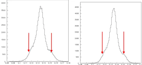
A.1 Figure A.3: The F.O.M. distribution in diﬀerent q_B × q × r bins from B^±→ ηK^±decay, The red arrows show the LR cut selections. . . 100

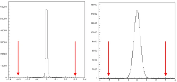
B.1 The translate function. First order diﬀerential is larger than zero when 0.2 < x < 1.0. Also give a better resolution in 0.8 < x < 1.0 and 0.2 < x < 0.4 after translated. . . 102 B.2 TheLR(left) and the translated LR(right) in B^±→ η(γγ)K^±

decay. The red line shows the signal and blue line stands for countinuum background. . . 103 B.3 Describe the translated LR of B^± → η(γγ)K^± countinuum

background with two Gaussian(left). Describe the translated LR of B^± → η(γγ)K^± signal with one Gaussian(right). . . 104

C.1 The modify M_bc(red) and typical M_bc(blue) in B^±→ η(γγ)K^± signal MC. Better resolution is provided by the modify M_bc. . 107 C.2 The modify Mbc(red) and typical Mbc(blue) in B^±→ η(π⁺π⁻π⁰)K^±(left)

and B⁺ → D⁰π⁺(right) signal MC. . . 107 C.3 The modify ∆E and typical M_bc scatter plot(left), ∆E and

modify M_bcscatter plot(right). Correlation is reduced in mod- ify M_bc. . . 108 C.4 The ∆E(left) and M_bc(right) distributions in B^±→ η(γγ)K^±

rare B background, The red one is from modify M_bc and blue one is typical M_bc. The modify M_bcprovide a better seperation between signal and rare B background. . . 109

(17)

C.5 The ∆E(left) and M_bc(right) distributions in B^±→ η(π⁺π⁻π⁰)K^± rare B background, The red one is from modify M_bc and blue one is typical M_bc. The modify M_bcprovide a better seperation between signal and rare B background. . . 109 C.6 The ∆E(left) and M_bc(right) distributions in B^±→ η(γγ)K^±

continuum background, The red one is from modify M_bc and blue one is typical Mbc. The distributions are same in two deﬁnition. . . 110

D.1 The ∆E plots in diﬀerent M_bcregions of B^± → η(γγ)K^±mode in true signal with(left) and without(right) normalization. . . 112 D.2 The ∆E plots in diﬀerent M_bcregions of B^± → η(γγ)K^±mode

in SCF with(left) and without(right) normalization. . . 112 D.3 The M_bcplots in diﬀerent ∆E regions of B^± → η(γγ)K^±mode

in true signal with(left) and without(right) normalization. . . 113 D.4 The M_bcplots in diﬀerent ∆E regions of B^± → η(γγ)K^±mode

in SCF with(left) and without(right) normalization. . . 113 D.5 The ∆E plots in diﬀerent Mbc regions of B → η(π⁺π⁻π⁰)K^±

mode in true signal with(left) and without(right) normalization. . . 114 D.6 The ∆E plots in diﬀerent M_bc regions of B → η(π⁺π⁻π⁰)K^±

mode in SCF with(left) and without(right) normalization. . . 114 D.7 The M_bc plots in diﬀerent ∆E regions of B → η(π⁺π⁻π⁰)K^±

mode in true signal with(left) and without(right) normalization. . . 115 D.8 The Mbc plots in diﬀerent ∆E regions of B → η(π⁺π⁻π⁰)K^±

mode in SCF with(left) and without(right) normalization. . . 115

(18)

E.1 The ∆E (left) and M_bc (right) 1-D ﬁt from signal MC (control sample). LR cut larger than 0.2 is applied. . . 117 E.2 The ∆E (left) and M_bc (right) 1-D ﬁt from real data (control

sample). LR cut larger than 0.2 is applied. The blue line shows the signal PDF, red for continuum background, and green for generic B background. . . 117 E.3 The fudge fators study in diﬀerent π⁰ momentum regions. . . 118

F.1 The M ax(likelihood)^likelihood in different branching fraction in B^± → η(γγ)K^± mode (top). The blue line is before smearing, and red line is after smearing with PDFs systematic error. And they overlap completely because the PDFs systematic error is very small. So we also show the effect in smearing with total systematic error (bottom). And it is a dome, we do not use the bottom one to calculate significance. . . 120 F.2 The M ax(likelihood)^likelihood in different A_CP in B^± → η(γγ)K^± mode

(top). And in B^± → η(γγ)π^± mode (bottom). The blue line is before smearing, and red line is after smearing with PDFs systematic error. And they overlap completely because the PDFs systematic error is very small. . . 121

G.1 The log(likelihood) distribution in diﬀerent branching fraction in B^±→ η(γγ)K^± mode. . . 122 G.2 The log(likelihood) distribution in diﬀerent branching fraction

in B^±→ η(π⁺π⁻π⁰)K^± mode. . . 123 G.3 The combined log(likelihood) in B^± → ηK^± mode. . . 123

(19)

List of Tables

1.1 The branching ratio in B → ηK^± decay is 2.33^+0.33_−0.34 in PDG . . 4

1.2 The branching ratio in B → ηπ^± decay is 4.07± 0.32 in PDG . 4 1.3 The branching ratio in B → ηKS⁰ decay is 1.15^+0.43_−0.38± 0.09 in PDG. . . 5

1.4 The branching ratio in η decay [PDG]. . . . 5

2.1 The parameters of the KEKB accelerator. . . 9

2.2 The detail of each sub-detector in the Belle detector. . . 12

2.3 Conﬁguration of the CDC sense wire and cathode strips [25]. . 17

2.4 Parameters of ECL [25]. . . 21

3.1 Summary of particle selection criteria . . . 27

4.1 The regions of missing mass of KSFW . . . 35

4.2 The ﬁsher distance for each M_miss bin. . . 35

4.3 The summary of expected signal in signal box for 2D ﬁt and 3D ﬁt in each decay mode. . . 39

(20)

4.4 The summary of ratio between feedacross backgrounds and ﬁtting yield. For example, if there are 1 signal yield in B^±→ η(γγ)π^± decay mode, the ﬁtter will force 0.08215 feedacross background in B^± → η(γγ)K^± decay mode. . . 45

5.1 The selection criteria of B⁺ → D⁰(K⁺π⁻π⁰)π⁺ . . . 51 5.2 The selection criteria of inclusive D⁰ → K⁺π⁻π⁰ . . . 51 5.3 The ﬁtting results of Fig. 3.1 and Fig. 3.2. The shape param-

eter of the PDFs are listed in Table 5.4. . . 53 5.4 The calibration factors. All units are MeV/c² for Mbc param-

eters and MeV for ∆E parameters. . . . 55

6.1 The wrong-tagging fraction w_l for tagged B⁰ and B⁰ in each r bin. . . . 58 6.2 The PDFs for M_bc, ∆E and translated LR 3-D ﬁt in B →

η(γγ)h modes. . . . 58 6.3 The PDFs for M_bc, ∆E and translated LR 3-D ﬁt in B →

η(π⁺π⁻π⁰)h modes. . . . 59 6.4 The poisson distribution mean for signal and background in

our ensemble test. . . 63 6.5 The poisson distribution mean for signal and background in

our ensemble test. . . 71

(21)

7.1 The LR cut eﬃciency for data and MC of the control sample. 81 7.2 The KID eﬃciency (%) and fake rate for B^± → ηK^± and

B^± → ηπ^±, here K^± and π^± come from B^± . Ratio = (Data/M C). . . . 83 7.3 The KID eﬃciency (%) for B → η(π⁺π⁻π⁰)h. The π^± eﬃ-

ciency comes from η. . . . 83 7.4 The summary of branching fractions systematics error (%) for

each mode. . . 85 7.5 The summary of ACP systematics error (%) for each mode. . 86

8.1 Summary table of branching fractions and other details for each decay mode. Detection efficiency ϵ_{ef f} including sub-decay branching fraction, yield, fit bias, significance (Sig.), measured branching fraction (B), and A_CP for the B→ ηh decays. Thre first errors are statistical and the second ones are systematic. . 87 8.2 Summary table of A_CP in each decay mode. . . 88 8.3 Summary table of continuum background A_CP in each decay

mode. All of them are less than 10% of statistical error in signal A_CP. . . 88 8.4 Summary table of yields of continuum background in each

decay mode. . . 88

A.1 Table A.1: The summarization ofLR cuts in each qB× q × r bins in B^± → ηK^± decay mode. . . 99

H.1 Summary table of ϵ_BB and r(ϵ_qq). . . 125

(22)

Chapter 1 Prologue

1.1 Standard Model

The Standard Model of particle physics (SM) [15] is a theoretical picture concerning the electroweak, electromagnetic, and strong interactions. The elementary particles are separated into four families, namely the quarks, leptons, gauge bosons and other bosons(Higgs boson). Quarks and leptons consist of six particles, split into three generations, And with the ﬁrst generation being the lightest, and the third the heaviest in quarks and charged leptons. Furthermore, gauge bosons are force carrying mediators in the three interactions.

The dynamics in Standard Model depend on 28 parameters, whose nu- merical values are established by experiment. The 28 parameters include 6 leptons mass, 6 quarks mass, 3 CKM mixing angle, 1 CKM CPV phase, 3 gauge coupling constant, 1 QCD vacuum angle, 1 Higgs quadractic coupling, 1 Higgs self-coupling strength, 3 PMNS mixing angle, 1 PMNS Dirac CPV phase, and 2 PMNS Majorana CPV phase .

(23)

Figure 1.1: The three generation quarks and leptons, with the gauge bosons in the rightmost column.

(24)

1.2 CP violation and CKM matrix

Parity(P) conservation is believed to be true before C.-S. Wu found the parity violation in the β decay in 1957. After that, people replace parity conservation to charge conjugation and parity (CP) conservation. But in 1964, the violation of CP symmetry was found in the decays of neutral K meson system by James Cronin and Val Fitch [18].

In Standard Model weak interaction is the only way that qaurks and leptons can change to anther type. And the ﬂavor changing of quark is described by



 d^′ s^′ b^′



 = V_CKM



 d s b



 =



 V_ud V_us V_ub V_cd V_cs V_cb Vtd Vts Vtb







 d s b



 , (1.1)

where the 3 × 3 unitary matrix is called CKM matrix or quark mixing matrix [19]. The CKM matrix can parameterized in several ways, one of the parameterization, called Wolfenstein’s parameterization, which transfer the CKM matrix in the form of an expansion in λ = sin θ_c, where θ_c is Cabibbo angle. And Wolfenstein’s parameterization has an advantage of giving four parameters in a same order.

V_CKM =



 1−^λ₂² λ Aλ³(ρ− iη)

−λ 1− ^λ₂² Aλ² Aλ³(1− ρ − iη) −Aλ² 1



 + O(λ⁴) , (1.2)

1.3 Motivation

Our motivation is to give branching ratios of B → ηh decays with about 50%

more data compare to the previous measurement in Belle. And in order to rise the significance we also going to 3-D fit instead of 2-D fit.

(25)

In SM, η and η^′ quark wave functions are linear combinations of ûu+dd√ 2 and ss. It is expected to enhance the B^± → η^′K^± decay amplitude but suppress the B^± → ηK^± decay amplitude. Thus, studying B^± → ηK^± may give us more information in η− η^′ mixing and B(B^± → η^′K^±) puzzle. Moreover, interference of different diagrams may provide a large direct CP asymmetry in B^± → ηK^± and B^± → ηπ^±. Therefore, the previous BaBar and Belle measurements give a CP asymmetry near to−30% in B^± → ηK^±decay. It’s very interesting and important to confirm the A_cp(ηK^±). And here shows the Feynman diagrams involved in our study.

We report the ﬁnal updated measurements of branching fractions and partial rate asymmetries for B decays to a pseudoscalar-pseudoscalar mesons with one η meason in the ﬁnal state. Our decay modes are considered:

η(γγ)K⁺, η(π⁺π⁻π⁰)K⁺, η(γγ)K⁰, η(π⁺π⁻π⁰)K⁰, η(γγ)π⁺, η(π⁺π⁻π⁰)π⁺ The data sample consists of 710 f b⁻¹ for data from Exps 7-65, corresponding to 772 million BB pairs. Here shows the braching ratios in B → ηh^± decay measured by pervious experiments in PDG.

Table 1.1: The branching ratio in B → ηK^± decay is 2.33^+0.33_−0.34 in PDG . Branching Ratio (10⁻⁶) Author TECN COMMENT

2.94^+0.39_−0.34 ± 0.21 Aubert 09AV BABR [1] e⁺e⁻→ Υ(4S) 2.21^+0.48_−0.42(stat)^±0.25_−0.18(syst) Wicht 08 BELL[2] e⁺e⁻→ Υ(4S) 1.9± 0.3^+0.2_−0.1 Chang 07B BELL[3] e⁺e⁻→ Υ(4S) 2.2^+2.8_−2.2 Richichi 00 CLE2[4] e⁺e⁻→ Υ(4S)

Table 1.2: The branching ratio in B → ηπ^± decay is 4.07± 0.32 in PDG . Branching Ratio (10⁻⁶) Author TECN COMMENT

4.00± 0.40 ± 0.24 Aubert 09AV BABR e⁺e⁻ → Υ(4S) 4.2± 0.4 ± 0.2 Chang 07B BELL e⁺e⁻ → Υ(4S) 1.2^+2.8_−1.2 Richichi 00 CLE2 e⁺e⁻ → Υ(4S)

(26)

Table 1.3: The branching ratio in B → ηKS⁰ decay is 1.15^+0.43_−0.38±0.09 in PDG.

Branching Ratio (upper limit) (10⁻⁶) Author TECN COMMENT 1.15^+0.43_−0.38 ± 0.09(< 1.8) Aubert 09AV BABR e⁺e⁻→ Υ(4S) (< 1.9) [ not used in PDG ] Chang 07B BELL e⁺e⁻→ Υ(4S)

Table 1.4: The branching ratio in η decay [PDG].

Decay mode Branching Ratio (%)

2 γ 39.31± 0.20

π⁺ π⁻ π⁰ 22.74± 0.28

Figure 1.2: Examples of Feynman diagrams involved in B^±→ ηK^± decay.

(27)

Figure 1.3: Examples of Feynman diagrams involved in B^±→ ηπ^± decay.

Figure 1.4: Examples of Feynman diagrams involved in B^± → ηKS⁰ decay.

(28)

Chapter 2 KEK B-Factory

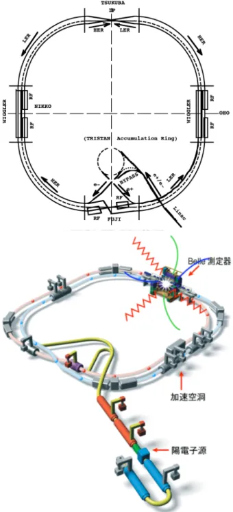
The KEK B-Factory (KEKB) [22] is an e⁺-e⁻ collider which located at the High Energy Accelerator Research Organization (KEK) in Tsukuba area, Ibaraki Prefecture, Japan. The construction of KEKB accelerator and detector started in April 1994. Operatoin was started at Dec. 1998 and truned oﬀ at June 30 2010. It’s main goal is to search for signatures of physics beyond the standard model through high-sensitivity measurements. It also presents the measurements of CP asymmetry in B meson decays. The re- sults of KEKB agree the prediction of KM model [19], and provided a strong experimental support for M. Kobayashi and T. Maskawa to win the 2008 Nobel Prize in Physics [24].

2.1 KEKB Accelerator

The KEKB accelerator is an two-rings, asymmetric, e⁺-e⁻collider. Which is based on the existing TRISTAN tunnel of 3 km circumference to construct the high energy ring (HER) and low energy ring (LER). The HER stores e⁻ and the LER stores e⁺. The energy of e⁺and e⁻is 3.5 and 8 GeV, and provide the center-of-mass energy of e⁺-e⁻ beams at the Υ(4S) resonance, and large number of B meson pairs can be produce via e⁺e⁻→ Υ(4S) → BB.

(29)

In KEKB accelerator electrons and positrons beam collide at a crossing angle of±11 mrad at the center of the BELLE detector. It not only allows su- perconducting RF cavity to be ﬁlled within the beam but also avoid parasitic collisions. The crossing angle also eliminate the need of the separation-bend magnets and reduces beam-related backgrounds in BELLE detector.

The main parameters of KEKB are summarized in Table 2.1, and Figure 2.1 shows the conﬁguration of the accelerator.

(30)

Table 2.1: The parameters of the KEKB accelerator.

Ring LER HER Unit

Energy E 3.5 8.0 GeV

Circumference C 3016.26 m

Luminosity L 1× 10³⁴ cm⁻²s⁻¹

Crossing angle θ_x ±11 mrad

Tune shifts ξ_x/ξ_y 0.039/0.052

Beta function at IP β_x^∗/β_y^∗ 0.33/0.01 m

Beam current I 2.6 1.1 A

Natural bunch length σ_z 0.4 cm

Energy spread σ_ε 7.1× 10⁻⁴ 6.7× 10⁻⁴

Bunch spacing s_b 0.59 m

Particles/bunch N 3.3× 10¹⁰ 1.4× 10¹⁰ Emittance ε_x/ε_y 1.8× 10⁻⁸/3.6× 10⁻¹⁰

Synchrotron ν_s 0.01∼ 0.02

Betatron tune ν_x/ν_y 45.52/45.08 47.52/43.08 Momentum compaction factor α_p 1× 10⁻⁴∼ 2 × 10⁻⁴

Energy loss/turn U₀ 0.81^†/1.5^†† 3.5 MeV

RF voltage V_c 5∼ 10 10∼ 20 MV

RF frequency f_RF 508.887 MHz

Harmonic number h 5120

Longitudinal damping time τ_ε 43^†/23^†† 23 ms

Total beam power P_b 2.7^†/4.5^†† 4.0 MW

Radiation power P_SR 2.1^†/4.0^†† 3.8 MW

HOM power P_HOM 0.57 0.15 MW

Bending radius ρ 16.3 104.5 m

Length of bending magnet l_B 0.915 5.86 m

†: without wigglers, ††: with wigglers

(31)

Figure 2.1: Schematic layout of KEKB from the top and side view.

(32)

2.2 Belle Detector

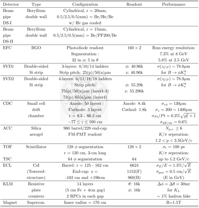
The Belle detector [25] is a collection of sub-detectors built around the interaction point of the KEKB accelerator. The coordinate system of the Belle detector is defined with the z-axis antiparallel to the e⁺ beam and the x-axias pointing inward, toward the center of the KEKB storage rings. It is often to use polar corrdinates(θ, ϕ,and r) with polar angle θ defined as the angle away from the z-axis. The Belle detector subsystems cover a full 2π in ϕ and three ranges in polar angle θ: the barrel region (34^◦ < θ < 127^◦), the forward endcap (17^◦ < θ < 34^◦), and the backward endcap(127^◦ < θ < 150^◦). Table 2.2 summarize the performance of the Belle detector and its sub-detectors, and Figure 2.2 shows the configuration of them in isometric and side view.

Figure 2.2: The structure of the Belle detector in isometric and side view. [26].

2.2.1 Beam Pipe

Since the multiple Coulomb scattering could aﬀects the track resolution, it is important to minimise the impact of the beampipe on particle trajectories with a thin material(low atomic number). So a beryllium beampipe was installed in the Belle Detector. The beam pipe is a dual layer cylinder with radii 20.0 mm and 23.0 mm, which thickness are 0.5 mm. The gap between these two beryllium walls provides a channel for helium gas, which is used as a coolant. In 2003, the original beampipe was replaced by a new one which

(33)

Table 2.2: The detail of each sub-detector in the Belle detector.

Detector Type Conﬁguration Readout Performance

Beam Beryllium Cylindrical, r = 20mm, pipe double wall 0.5/2.5/0.5(mm) = Be/He/Be

DS-I w/ He gas cooled

Beam Beryllium Cylindrical, r = 15mm, pipe double wall 0.5/2.5/0.5(mm) = Be/PF200/Be DS-II

EFC BGO Photodiode readout 160× 2 Rms energy resolution:

Segmentation : 7.3% at 8 GeV

32 in ϕ; 5 in θ 5.8% at 2.5 GeV

SVD1 Double-sided 3-layers: 8/10/14 ladders ϕ: 40.96k σ(z_CP)∼ 78.0µm Si strip Strip pitch: 25(p)/50(n)µm z: 40.96k for B → ϕKs⁰

SVD2 Double-sided 4-layers: 6/12/18/18 ladders σ(zCP)∼ 78.9µm

Si strip Strip pitch: ϕ: 55.29k for B → ϕKs⁰

75(p)/50(n)µm (layer1-3) z: 55.296k 73(p)/65(n)µm (layer4)

CDC Small cell Anode: 50 layers Anode: 8.4k σrϕ= 130µm

drift Cathode: 3 layers Cathod: 1.8k σz= 200∼ 1400µm

chamber r = 8.3 - 86.3 cm σP t/P t = 0.3%√

p²_t+ 1

−77 ≤ z ≤ 160 cm σ_dE/dx= 0.6%

ACC Silica 960 barrel/228 end-cap N_p.e.≥ 6

aerogel FM-PMT readout K/π seperation:

1.2 < p < 3.5GeV/c

TOF Scintillator 128 ϕ segmentation 128× 2 σ_t = 100 ps

r = 120 cm, 3-cm long K/π seperation:

TSC 64 ϕ segmentation 64 up to 1.2 GeV/c

ECL CsI Barrel: r = 125 - 162 cm 6624 σE/E = 1.3%/√

E

(Towered- End-cap: z = 1152(F) σpos= 0.5 cm/√

E

structure) -102 cm and +196cm 960(B) (E in GeV)

KLM Resistive 14 layers θ: 16k ∆ϕ = ∆θ = 30mr

plate (5 cm Fe + 4cm gap) ϕ: 16k for K_L

counters 2 RPCs in each gap ∼ 1% hadron fake

Magnet Supercon. Inner radius = 170 cm B=1.5T

(34)

inner radius is 15.0 mm. The cross-section of the beam pipe is shown in Figure 2.3. The arrangment of the beam pipe and these masks are in Figure 2.4.

Figure 2.3: The cross-section of the beam pipe at the IP [25].

Figure 2.4: The structure of the beam pipe and horizontal masks [25].

2.2.2 Silicon Vertex Detector (SVD)

The primary goal of the SVD is to measure the B meson decay vertex, which is essential for time-dependent CP V study. SVD1 was a three layers Double- sided Silicon Detector(DSSD) in a barrel-only design(23^◦ < θ < 139^◦),

(35)

comprising of 8, 10, and 14 ladders in the inner, middle, and outer layers, respectively. Each ladder is constructed from two joined half-ladders. In summer 2003, the SVD 2 was replaced by a new SVD system (SVD 2). The SVD 2 consists four layers consisting of 6, 12, 18, and 18 ladders from the innermost layer, respectively. And covers more percentage of full solid angle then SVD I (17^◦ < θ < 150^◦).

Figure 2.5: Conﬁguration of SVD [25].

2.2.3 Extreme Forward Calorimeter (EFC)

The Extreme Forward Calorimeter (EFC) extend the polar angle coverage in both extreme forward and backward regions (6.4^◦ < θ < 11.5^◦ and 163.3^◦ < θ < 171.2^◦) which do not cover by ECL. It is useful to improve the experimental sensitivity in some special decay channels such as B → τν decay. The main material of EFC is the radiation-hard BGO (Bismuth Ger- manate, Bi₄Ge₃O₁2) crystal calorimeter due to their higher radiation toler- ance.

In fact, the EFC has never been used in decay reconstruction. However, its geometric location allows it to act as a beam mask to reduce radiation

(36)

backgrounds to the CDC. In addition, EFC is used for online luminosity and background monitoring. The structure of the cone-like EFC are shown in Fig. 2.6.

Figure 2.6: Side view of forward EFC (left) and isometric view of the forward and backward EFC detectors (right) [25].

2.2.4 Central Drift Chamber (CDC)

The Central Drift Chamber (CDC) with inner(outer) radius 103.5(874) mm and covers the angular range from 17^◦ < θ < 150^◦. The CDC has a total of a total of 8400 drift cells placed on 50 cylindrical layers. Each of its 8400 drift cells consists of a sense wire, held at a high voltage(2.35 kV), surrounded by field wires, held at low voltage. The CDC is filled with a 50% helium, 50% ethane (C₂H₆) mixture.The configuration of CDC can be seen in Fig.

2.7. The CDC is used to provide the information of momentum and dE/dx (for particle identiﬁcation) from charged particles. Charged particles passing through the gas ionize electrons, and the ionized electrons drift forwards to the sense wire. Therefore, the track information is collected.

The particle transverse momentum can be determined from the curvature of the helix(r) as pT = 0.3Br, where pT is in units of GeV/c, B is the magnetic ﬁeld in Tesla, and r is in meters. More details of CDC are summarized in Table 2.3, and the conﬁguration of CDC drift cells are shown in Fig. 2.8.

(37)

Figure 2.7: Overview of CDC structure [25]. The lengths in the ﬁgure are in units of mm.

2.2.5 Aerogel Cherenkov counter system (ACC)

The Aerogel Cherenkov counter (ACC) is used to provide particle identiﬁca- tion information to distinguish K^± from π^± in high monmentum range (1.2 GeV/c∼ 4.0 GeV/c) by Cherenkov radiation. Cerenkov radiation is emitted if the velocity of a charged particle exceeds the speed of light in medium, n > _β¹ = √

1 + (^m_p)², where m and p are the mass and momentum of the charged particle, and n is the refractive index of the material. Therefore, it is possible to distinguish kaons from pions by selecting a material in which pions will emit Cherenkov light, but kaons will not.

The ACC can be separated into barrel and forward end-cap part. The barrel part is consists of 960 counter modules, and 228 in the end-cap part.

The counter module is a thin aluminum box containing two principal components: a stack of ultralight aerogel with index of refraction (n = 1.010, 1.013, 1.015, 1.020, 1.028 and 1.030), and one or two ﬁne mesh photomultipler tubes (PMTs) to detect Cherenkov light. Figure 2.10 shows the conﬁguration of ACC, and Figure 2.11 shows the counter module in the barrel and end-cap

(38)

Table 2.3: Conﬁguration of the CDC sense wire and cathode strips [25].

Superlayer No. of Channels Radius Stereo angle (mrad) type layers per layer (mm) [strip pitch (mm)]

Cathode 1 64(z)×8(ϕ) 83.0 [8.2]

Axial 1 2 64 88.0−98.0 0.

Cathode 1 80(z)×8(ϕ) 103.0 [8.2]

Cathode 1 80(z)×8(ϕ) 103.5 [8.2]

Axial 1 4 64 108.5−159.5 0.

Stereo 2 3 80 178.5−209.5 71.46−73.75

Axial 3 6 96 224.5−304.0 0.

Stereo 4 3 128 322.5−353.5 -42.28−-45.80

Axial 5 5 144 368.5−431.5 0.

Stereo 6 4 160 450.5−497.5 45.11−49.36

Axial 7 5 192 512.5−575.5 0.

Stereo 8 4 208 594.5−641.5 -52.68−-57.01

Axial 9 5 240 656.5−719.5 0.

Stereo 10 4 256 738.5−785.5 62.10−67.09

Axial 11 5 288 800.5−863.0 0.

parts.

2.2.6 Time-of-Flight Counters (TOF)

The Time of Flight Counter (TOF) provide particle identiﬁcation information to distinguish charged kaons from pions in the low momentum region(less then 1.2 GeV/c).

The TOF covers the agnle range region of 34^◦ < θ < 120^◦, and it consists of 128 TOF counters and 64 trigger scintillation counters (TSC). One TOF/TSC modules is consists of two trapezoidally shaped TOF and one TSC counters. Signals could be read by ﬁne-mesh-dynode photomultiplier tubes (FM-PMT) which is mounted directly on the TOF and TSC scintillation counters and placed in a magnetic ﬁeld of 1:5 T. Figure 2.12 shows a TOF/TSC module geometry..

(39)

Figure 2.8: Cell structure (left) and the cathode sector conﬁguration (right) [25].

In TOF, the mass m of the charged particle is calculated from the follow- ing formula:

M_track² = ( 1

β² − 1 )

P² =

((cT_obs^twc Lpath

)2

− 1 )

P² , (2.1)

where T_obs^twc is the time walk correction on the measured FM-PMT signal time to get a precise observed time, and L_path(P ) stands for the path length (momentum) obtained from the CDC track. Fig. 2.13 shows the mass distri- bution for momenta below 1.2 GeV/c.

For each charged track, the CDC, ACC and TOF information are are combined to give a likelihood ratio to the particle identiﬁcation, mainly for the separation of protons/kaons/pions. Fig. 2.14 shows a plot that indicate the regions in which they work well in distinguishing charged particles.

2.2.7 Electromagnetic Calorimeter (ECL)

The Electromagnetic Calorimeter (ECL) is mainly used to detect the energy and position of photons from B meson decays by measuring electromagnetic

(40)

Figure 2.9: The plot of dE/dx and particle momentum, together with the expected truncated mean [25].

showers. And the photons momentum could be caluate with the photons’

mother’s decay point or IP. Combining the ECL information and dE/dx information in CDC and light yield in ACC, the ECL can also provide nice electron idnetiﬁcation. Figure 2.15 shows the conﬁguration of ECL.

High energy incident electron or photon causes an electromagnetic shower when interacting with a material. If the material is doped with a ﬂuor, the ionization energy losses from the shower are converted into visible light, which can be measured by a photodetector. Thus, cesium iodide crystals, doped with thallium as a ﬂuor (CsI(Tl)), are chosen. The ECL consists of 8,736 CsI(Tl) crystals shaped in a half-tower and point to the IP. The size of crystals range from 55 × 55 mm² (front face) and 82 × 82 mm² (rear face) for barrel part, and vary from 44.5 to 70.8 mm and from 54 to 82 mm, respectively in end-cap part. The length of each crystal is chosen to be 30 cm (16.2X₀). The whole ECL is comprised of a barrel section with 3m in length and 1.25m inner radius. And cover the polar angle region of 17^◦ < θ < 150^◦, the total covred solid-angle is 91% of 4π, other details of ECL can be seen in Table 2.4.

(41)

Figure 2.10: The arrangement of ACC in the Belle detector [25].

Figure 2.11: Schematic drawing of a typical ACC counter module: (a) barrel and (b) end-cap ACC [25].

2.2.8 K

L

and Muon Detector (KLM)

The KL and Muon Detector (KLM), which covering the polar angle region from 20^◦ to 155^◦, is located outside the solenoid and designed to detect K_L⁰ and µ^± particle with enough momentum to reach the KLM, P > 0.6GeV /c.

The KLM consists of 15 (14) layers of glass-electrode-resistive plate counters (RPCs) and 14 (14) layers of 4.7 cm-thick iron plates in the octagonal barrel region (the forward and backword end-caps). Those multiple layers of charged particle detectors and iron allow discrimination between muons and charged hadrons (π^±, K^±) based upon their range and transverse scattering.