GPE: A Grid-based Population Estimation Algorithm for
Resource Inventory Applications over Sensor Networks
*JIUN-LONG HUANG, SHIH-CHUAN CHIUAND XIN-MAO HUANG+
Department of Computer Science National Chiao Tung University
Hsinchu, 300 Taiwan
E-mail: {jlhuang; scchiu}@cs.nctu.edu.tw
+Department of Computer Science and Information Engineering Aletheia University
Taipei, 251 Taiwan E-mail: [email protected]
The growing advance in wireless communications and electronics makes the de-velopment of low-cost and low-power sensors possible. These sensors are usually small in size and are able to communicate with other sensors in short distance wirelessly. A sensor network consists of a number of sensors which cooperate with one another to ac-complish some tasks. In this paper, we address the problem of resource inventory appli-cations, which means a class of applications involving population calculation of a spe-cific object type. To reduce energy consumption, each sensor only reports the number of the sensed objects to the server, and the server will estimate the number of the sensed objects according to the received reports of all sensors. To address this problem, we de-sign in this paper a population estimation scheme, called algorithm GPE (standing for Grid-based Population Estimation), to estimate the numbers of the sensed objects. Sev-eral experiments are conducted to measure the performance of algorithm GPE. Experi-mental results show that algorithm GPE is able to obtain close approximations of the numbers of the sensed objects. In addition, experimental results also show that algorithm GPE is more scalable, and hence, is more suitable than prior schemes for practical use. Keywords: population estimation, resource inventory, sensor network, energy conserva-tion, estimation algorithm
1. INTRODUCTION
The growing advance in wireless communications and electronics makes the devel-opment of low-cost and low-power sensors possible. These sensors are usually small in size and are able to communicate with other sensors in short distance wirelessly. A sensor network consists of a number of sensors which cooperate with one another to accomplish some tasks [1]. Sensors can be deployed either in a random or in a predetermined manner. Since being self-organized, sensors are able to form a sensor network automatically. Due to the characteristics of wireless communication and configuration-free deployment, sen-sor networks are suitable for various application areas including inventory management, product quality monitoring and disaster area monitoring [1, 2]. Hence, sensor networks Received March 14, 2007; revised June 7 & November 9, 2007; accepted December 27, 2007.
Communicated by Chung-Ta King.
* The preliminary version of this work has been presented at International Conference on Mobile Ad Hoc and
Sensor Networks, 13-15 December, 2005, Lake View Hotel, Wuhan, China.
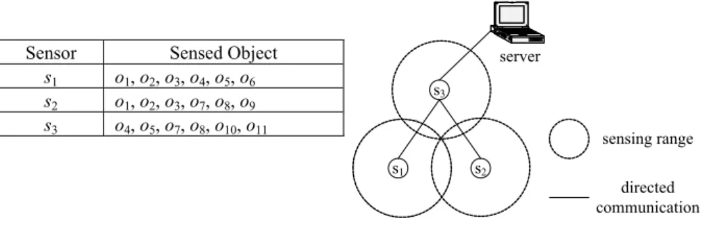
Sensor Sensed Object
s1 o1, o2, o3, o4, o5, o6
s2 o1, o2, o3, o7, o8, o9
s3 o4, o5, o7, o8, o10, o11
have attracted a significant research attention, including hardware and operating system design [3, 4], localization [5, 6], data aggregation methods [7-9] and applications of sen-sor networks [10, 11].
Resource inventory, in this paper, is defined as a class of applications involving population calculation of a specific object type. To achieve this, a number of sensors are deployed in a flat surface and each sensor is able to sense the number of objects within its sensing region. These sensors then form a sensor network so that users are able to query the number of objects sensed by the sensor network via a server. For the sake of simplicity, we use “object number” to indicate the number of objects sensed by a sensor network.
Since the sensors may be deployed randomly, the sensing regions of these sensors may overlap with one another. This phenomenon results in the difficulty of obtaining the exact object number due to the reason that one object may be sensed by more than one sensor. Suppose that each object has a unique identity. To calculate exact object numbers, each sensor should get the identities of all objects in its sensing region and send these identities to the server via a sink. After removing redundant identities, the server can get the exact object number by counting the number of remaining identities.
Sensors are usually powered by batteries. Therefore, energy conservation becomes an important issue in the design of sensor networks [12, 13]. As mentioned in [14], the energy consumption for a sensor to transmit and receive a message is in proportion to the length of the message. To reduce power consumption, the removal of redundant identities should be performed in an in-network manner.
s3 s1 s2 sensing range directed communication server
Fig. 1. An example scenario.
We use the example scenario in Fig. 1 to show the effect of in-network redundancy removal. When in-network redundancy removal is not performed, s1, s2 and s3 will report {o1, o2, o3, o4, o5, o6}, {o1, o2, o3, o7, o8, o9} and {o4, o5, o7, o8, o10, o11}, respectively, to the server. After receiving these reports, the server removes redundant identities and re-ports that there are 11 objects sensed by the sensor network. Consider the case that in-network redundancy removal is performed. After receiving the reports of s1 and s2, s3 first removes redundant identities in the reports of s1, s2 and the list of objects sensed by s3, and then reports {o1, o2, o3, o4, o5, o6, o7, o8, o9, o10, o11} to the server. Finally, the server reports that there are 11 objects sensed by the sensor network. It is obvious that in- network redundancy removal is able to reduce the power consumption of the sensor net-work by reducing the lengths of messages.
There are some scenarios that energy conservation is of the highest priority and knowing only estimated object number is useful enough. Consider the scenario of long- term inhabitant monitoring. Some scientists deploy several sensors in a wild field to ob-serve the number of some species of animals. We assume that the individual animals can be distinguished at the sensor by voice signatures, visual features, or pre-implanted arti-ficial identifications (RFID for example) [15]. Since changing the batteries of the sensors is quite difficult, to facilitate long-term monitoring, energy-conservation is of the highest priority and the obtained object number is not necessary to be exact.
In view of this, Lin et al. suggested in [15] that each sensor only reports the number of the sensed objects to the server. In the example scenario in Fig. 1, s1, s2 and s3 only send, respectively, {s1:6}, {s2:6} and {s3:6} to the server. For convenience, we name the scheme proposed in [15] as scheme SDARIA (i.e., the acronym of the title of [15]) in the rest of this paper. The amount of lengths of messages produced in in-network redundancy removal is 23 units, while the amount of lengths of messages produced by scheme SDARIA is 6 units. Since the energy consumption for a sensor to transmit and receive a message is in proportion to the length of the message, the energy saving of scheme SDARIA over in-network redundancy removal in this example is around 23-623 ≈ 73.91%.
After receiving all reports, the server will estimate the object number according to the received reports. To achieve this, they proposed two algorithms to calculate the lower bounds and the upper bounds of the exact object numbers based on the received reports. Although being shown to be able to conserve much energy than other schemes, scheme SDARIA has the following drawbacks.
1. The time complexity of the lower bound calculation algorithm is high.
The time complexity of the lower bound calculation algorithm in scheme SDARIA is O(1.2226n) where n is the number of sensors. Such high complexity makes scheme SDARIA not suitable for practical use.
2. The obtained lower bounds and upper bounds are not informative.
In our experiments, the upper bounds obtained by scheme SDARIA are around 190%- 300% of the exact numbers, while the lower bounds are around 60%-80% of the exact numbers. Such high error rates make users not able to get enough information about the exact object numbers.
In view of this, we design in this paper a population estimation algorithm, called algorithm GPE (standing for Grid-based Population Estimation), for the server to esti-mate the object numbers based on the received reports. Similar to scheme SDARIA, all sensors only report the number of the sensed objects to the server. To estimate the num-ber of the sensed objects, algorithm GPE first partitions the flat surface into several dis-joint grids, and identifies overlapping grids of each sensor. Algorithm GPE then esti-mates the object number of each grid, and finally estiesti-mates the object numbers according to the estimated object number of each grid. Several experiments are conducted to meas-ure the performance of algorithm GPE. The experimental results show that algorithm GPE is able to obtain close approximations of object numbers. In our experiments, the approximations of algorithm GPE are around 95%-115% of the exact object numbers. In addition, algorithm GPE is more scalable than scheme SDARIA. These features make algorithm GPE more suitable for practical use. Finally, we have proposed a two-phase
framework to strike a balance between estimation accuracy and energy-conservation by using scheme ADARIA and algorithm GPE in turn.
The rest of this paper is organized as follows. Section 2 gives a description of re-source inventory applications and an overview of scheme SDARIA. The design of algo-rithm GPE is given in section 3. Section 4 shows the performance study of algoalgo-rithm GPE and discusses some possible combined use of scheme SDARIA and algorithm GPE. Finally, section 5 concludes this paper.
2. PRELIMINARIES 2.1 System Architecture
Similar to [15], the system architecture of resource inventory applications is shown in Fig. 2. To calculate the number of objects, a number of sensors are deployed in a flat surface and each sensor is able to sense the objects within its sensing region. These sen-sors then form a sensor network and users are able to query the number of objects via a server. For energy conservation, each sensor only reports the number of the sensed ob-jects to the server when the server requests all sensors to report their sensing status. We assume that the server is able to get the sensing regions of all sensors. The location of each sensor can be obtained from manual measurement by human or automatic meas-urement by sensors when they are equipped with GPS [16]. We also assume that the sensing region of each sensor is determined as a circle centered by the sensor’s location. The radius of the circle is called the sensing radius of the sensor. For simplicity, we as-sume that each sensor has the same sensing radius r and let n denote the number of sen-sors. For better readability, the symbols used is listed in Table 1.
Overlap Graph Server Estimated Population 3 8 12 8 15 9 8 15 12 9 3 8 Sink Sensing Ranges Fig. 2. System architecture. Table 1. Description of symbols.
Symbol Description
n Number of sensors
r Sensing radius
G Overlap graph
V Vertices in the overlap graph
E Edges in the overlap graph α Grid size ratio
2.2 Related Work
Basically, scheme SDARIA comprises the following two phases.
• Report collection phase: In report collection phase, each sensor reports the number of the sensed objects to the server via the sink. After receiving the reports of all sensors, the server transforms the received reports into the corresponding overlap graph G = {V, E}, where V and E are, respectively, the sets of vertices and edges in G. The transfor-mation procedure is as follows. Each sensor is modelled as a vertex, and the weight of the vertex is the number of objects sensed by the corresponding sensor. In addition, there is an edge between two sensors if these two sensors’ sensing regions overlap. Af-ter building the overlap graph, the server then enAf-ters population estimation phase. • Population estimation phase: In population estimation phase, the server estimates the
object number according to the overlap graph G. In scheme SDARIA, two algorithms are proposed to calculate the upper bound and the lower bound, respectively, of the ex-act object number, and these two bounds are taken as the results of scheme SDARIA.
In scheme SDARIA, lower bound calculation is modelled as the maximal inde-pendent set problem. However, according to [17], the fastest algorithm for maximal in-dependent set problem is of complexity O(1.2226n) where n is the number of sensors. Thus, the lower bound calculation is not scalable. On the other hand, upper bound calcu-lation is modelled as finding a subset of V which includes solely the vertices whose sensing regions cannot be replaced by the combinations of other vertices’ sensing regions. Interested readers can refer to [15] for details. In our experiments, the obtained upper bounds are around 190%-300% of the exact object numbers, and the lower bounds are around 60%-80% of the exact object numbers. Such high error rates make users not able to get enough information about the exact object numbers. Due to the above drawbacks, scheme SDARIA is suitable for practical use.
3. GPE: GRID-BASED POPULATION ESTIMATION
In algorithm GPE, the monitored region is partitioned into several non-overlapping grids. The length and width of each grid are set to α × r, where the value of α is called grid size ratio and r is the sensing region of each sensor. We will discuss how to deter-mine the value of α in section 4.2. Consider the sensing region of a sensor shown in Fig. 3. A grid g is called the full grid of a sensor s if all the area of grid g is covered by the sensing region of sensor s. Similarly, a grid g is called the partial grid of a sensor s if only part of the area of grid g is covered by the sensing region of sensor s. A grid g is called the overlapping grid of sensor s if grid g is a full or a partial grid of sensor s. In Fig. 3, the full and partial grids of the sensor are marked as ‘F’ and ‘P,’ respectively.
To facilitate the estimation of the exact object numbers, we have the following as-sumptions.
1. The objects sensed by sensor s are uniformly distributed in the sensing region of sensor s. 2. The objects in a grid g are uniformly distributed in the area of grid g.
P P P P P F P P P F F F P P P F P P P P P Grid Sensing Region (x1,y1) d (0,0) gs
Fig. 3. Full and partial grids. Fig. 4. An example object distribution. The reasons that we make these two assumptions are as follows.
1. The assumption that the objects in the sensing region are uniformly distributed is used only as an initial setting. Algorithm GPE will automatically adjust the distribution of objects in a sensing region according to the numbers of objects sensed by all sensors. At the end of algorithm GPE, the objects in each sensing region will not be considered as uniformly distributed.
Consider the example shown in Fig. 5. As shown in Fig. 5 (b), algorithm GPE first as-sumes that the objects in the sensing region of sensor s1 are distributed uniformly. Thus, the numbers of the objects in the grids of sensor s1 are equal. At the end of algorithm GPE, the distribution of the objects in each sensing region is adjusted according to the numbers of objects in each sensing region. As a result, in Fig. 5 (d), the numbers of the objects in the grids of sensor s1 become different.
2. Algorithm GPE indeed relies on the assumption that the objects within a grid are tributed uniformly. We believe that when the grid size becomes small enough, the dis-tribution of objects in a grid will become close to uniform disdis-tribution. Thus, algo-rithm GPE becomes more accurate when grid size is set to be smaller. We use the fol-lowing lemma to explain this assumption. Moreover, this intuition conforms to the experimental result shown in Fig. 7 (a).
Sensing region of sensor s
Grid g
Overlapping region
Grid g
Sensing region of sensor s
(a) Full grid. (b) Partial grid. Fig. 5. Overlapping between grid g and the sensing region of sensor s.
Lemma 1 Suppose that the objects are distributed normally. When the grid size
be-comes smaller, the distribution of objects in a grid will become closer to uniform distri-bution.
Proof: Consider the example shown in Fig. 4. Without lost of generality, we assume that
the grid g lies in Quadrant I. Let the coordinate of the bottom-left point in g be (x1, y1) and the grid size be d. Let pdf(x) be the probability that the x-coordinate of an object is x. Since the objects are distributed normally, we have
(
) (
)
(
) (
)
2 2 (1 ) ( +1 ) 2 2 2 2 2 2 (1 ) (1 ) 2 2 2 2 2 2 2 (1 ) (1 ) 2( ) 2 2 2 2 2 2 1 1 0 0 0 0 lim[ ( ) ( )] 1 1 lim 2 2 1 lim 2 1 lim 2 1 2 x x d x x d x x x d d d d d d pdf x pdf x d e e e e e e e μ μ σ σ μ μ σ σ μ μ μ σ σ σ σ π σ π σ π σ π σ − − − + − − − − − − → − − → − − → − − → − + ⎡⎛ ⎞ ⎛ ⎞⎤ = ⎢⎜⎜ ⎟ ⎜⎟ ⎜− ⎟⎟⎥ ⎢⎝ ⎠ ⎝ ⎠⎥ ⎣ ⎦ ⎡ ⎤ = × ⎢ − ⎥ ⎣ ⎦ ⎡ ⎤ = × ⎢ − ⎥ ⎣ ⎦ = 2 1 2 2 2( ) 2 2 ( ) 2 0 lim 1 0. x d d x d e e μσ μ σ π − − − − − → ⎡ ⎤ × × ⎣ − ⎦ =The above result shows that pdf(x1 + d) becomes closer to pdf(x) when d becomes closer to zero. Since probability density function is monotonic decreasing when x > 0,
pdf(x1 + d′), d′ ≤ d is close to pdf(x) when d is close to zero. With similar method, we can also show that when y > 0, pdf(y1 + d′), d′ ≤ d becomes closer to pdf(y) when d becomes closer to zero. Thus, with smaller grid size, the distribution of objects in a grid will be-come closer to uniform.
Let g.Area be the area of grid g, s.Area be the area of the sensing region of sensor s and s.ObjNo be the number of objects sensed by s. Then, according to these assumptions, we have the following lemma.
Lemma 2 Consider the case that a grid g overlaps the sensing region of a sensor s. Suppose that sensor s expects that there are g.ObjNo objects in grid g. Then, we have
. . . . . g Area g ObjNo s ObjNo s Area = × (1)
Proof: Since g overlaps the sensing region of s, by definition, g is either a full grid or a
partial grid of s. Consider the case shown in Fig. 5 (a) that g is a full grid of s. According to assumption 1, it is obvious that the ratio between the object number in g and the object number sensed by s is equal to the ratio between the area of g and the area of the sensing region of s. Thus, we have
. .
.
. .
g ObjNo g Area
s ObjNo = s Area
. . . . . g Area g ObjNo s ObjNo s Area = ×
Thus, Eq. (1) is true when g is a full grid of s.
We next consider the case shown in Fig. 5 (b) that g is a partial grid of s. Let OA.Area be the area of the overlapping region of grid g and the sensing region of sensor s and
OA.ObjNo be the number of objects in this overlapping region expected by sensor s.
Ac-cording to assumption 1, we have
. .
.
. .
OA ObjNo OA Area
s ObjNo = s Area
By rewriting the above equation, we have . . . . . OA Area OA ObjNo s ObjNo s Area = × (2)
According to assumption 2, we have
. .
.
. .
OA ObjNo OA Area
g ObjNo = g Area
By rewriting the above equation, we have . . . . . g Area g ObjNo OA ObjNo OA Area = ×
After rewriting the above equation by substituting the right hand side of Eq. (2) for
OA.ObjNo, we have . . . . . . . . . . g Area OA Area g ObjNo s ObjNo OA Area s Area g Area s ObjNo s Area ⎛ ⎞ = ×⎜ × ⎟ ⎝ ⎠ = ×
Thus, Eq. (1) is true when g is a partial grid of s.
As a result, this lemma is proven since Eq. (1) is true when g is a full grid or a par-tial grid of s.
Note that these assumptions are made only to guide the design of algorithm GPE, and are not the limitations of algorithm GPE. They will be relaxed in the experiments in section 4.
The procedure of algorithm GPE is as follows. Initially, each sensor is marked as UNSELECTED. Algorithm GPE is an iterative algorithm and selects one sensor marked as UNSELECTED in each iteration. Consider the case that sensor s is selected. Accord- ing to Lemma 2, sensor s suggests that g Areas Area.. ×s ObjNo. objects are in each of its over-
lapping grids. Finally, sensor s is marked as SELECTED. Algorithm GPE repeats the above procedure until all sensors are marked as SELECTED. Since the expected object number in grid g may be suggested by several sensors, the expected object number in grid g is determined as the average of possible object numbers suggested by all sensors. Finally, the estimated object number is determined as the summation of the expected object numbers of all grids. The algorithmic form of algorithm GPE is as follows.
Algorithm GPE
1: for each grid g do /* Initialization */ 2: g.AvgObjNo ← 0
3: g.SensorNo ← 0 4: end for
5: Mark all sensors as UNSELECTED
6: while (at least one sensor is marked as UNSELECTED) do
7: Pick one sensor which is marked as UNSELECTED 8: overlap ← overlap grids of sensor s
9: for each grid g in overlap do
10: expectation = g Areas Area.. ×s ObjNo.
11: g AvgObjNo. ←g SensorNo. 1 +1×( .g AvgObjNo g SensorNo expectation* . + ) 12: g.SensorNo ← g.SensorNo + 1
13: end for
14: Mark sensor s as SELECTED 15: end while
16: total ← 0 17: for each grid g do
18: total ← total + g.AvgObjNo 19: end for
20: return total
Since the width and the length of each grid are set to α × r, the number of grids in the flat surface is proportional of α12, while the number of overlapping grids of each sensor
is also in proportion to α12. Since being dominated by the loop in lines 6-15, the time
complexity of algorithm GPE is O(αn2) where n is the number of sensors. Finally, we
use the following example to illustrate the execution of algorithm GPE.
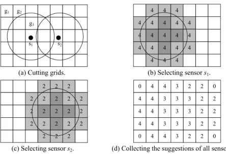
Example 1: Consider a sensor network consisting of two sensors, sensor s1 and sensor s2, which sense 50 and 25 objects, respectively. The locations of these sensors are shown in Fig.6 (a). The value of α is set to 0.5. Thus, the server partitions the monitored field into 35 non-overlapping grids and marks sensor s1 and sensor s2 as UNSELECTED. Since the width and the length of each grid g are α × r, we have g.Area = (α × r)2. In addition, we also have s.Area = π × r2. Thus, .
. g Area s Area is 2 2 2 2 . ( ) 0.5 0.08. . 3.1415... g Area r s Area r α α π π × = = = ≈ ×
Suppose that s1 is selected. According to Lemma 2, s1 expects each of its overlap- ping grids is of g Areas Area.. × s.ObjNo = 0.08 × 50 = 4 objects. The server marks sensor s1 as SELECTED. The server then selects sensor s2. Similarly, the server determines that sen-sor s2 expects that there are 0.08 × 25 = 2 objects in each overlapping grid of sensen-sor s2.
After selecting all sensors, the server then calculates the estimated object number in each grid. We use three grids, g1, g2 and g3, to demonstrate the calculation. Since grid g1 does not overlap the sensing region of each sensor, the server determines that there is no object in grid g1. Grid g2 is only covered by the sensing region of sensor s1. The server determines that there are four objects in grid g2 due to the reason that sensor s1 suggests that there are four objects in each overlapping grid of sensor s1. Since sensor s1 and s2 suggest there are, respectively, four and two objects in grid g3, the server determines that there are 4 2+2 =3 objects in grid g3. The result of this step is shown in Fig. 6 (d). Finally, the server summarizes the estimated object numbers of all grids and reports that there are 93 objects in the monitored field.
g1 g2 g3 s1 s2 4 4 4 4 4 4 4 4 4 4 4 4 4 4 4 4 4 4 4 4 4
(a) Cutting grids. (b) Selecting sensor s1. 2 2 2 2 2 2 2 2 2 2 2 2 2 2 2 2 2 2 2 2 2 0 4 4 3 2 4 4 3 3 3 4 4 3 3 3 4 4 3 3 3 0 4 4 3 2 2 2 2 2 2 0 2 2 2 0 (c) Selecting sensor s2. (d) Collecting the suggestions of all sensors.
Fig. 6. A running example.
4. PERFORMANCE EVALUATION 4.1 Simulation Model
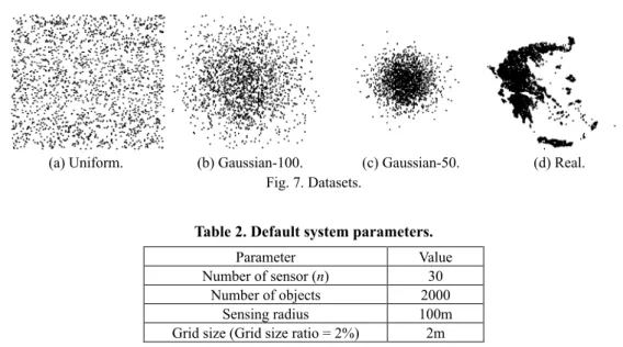
Similar as [15], the sensors are uniformly placed in to a 500m × 500m flat surface and the sensing radius of each sensor is set to 100m. We use GSTD tool [18] to generate the synthetic datasets used in this simulation. We synthesize the locations of objects by three distributions: uniform distribution, Gaussian distribution with standard deviation 100 and Gaussian distribution with standard deviation 50, and they are shown in Figs. 7 (a)-(c), respectively. In addition to synthetic datasets, we also use real spatial dataset
(a) Uniform. (b) Gaussian-100. (c) Gaussian-50. (d) Real. Fig. 7. Datasets.
Table 2. Default system parameters.
Parameter Value Number of sensor (n) 30
Number of objects 2000
Sensing radius 100m
Grid size (Grid size ratio = 2%) 2m
which contains the locations of 5922 cities and villages of Greece [19]. We normalize these locations into the flat surface, and the normalized result is shown in Fig. 7 (d). Since focusing on population estimation phase, in data aggregation phase, algorithm GPE adopts the data aggregation method used in scheme SDARIA. In addition to algorithm GPE, we also implement scheme SDARIA for comparison purposes. We implement both schemes in C++ and the simulation is executed in a PC with one Pentium III 500MHz CPU and 512MB memory. The default system parameters are listed in Table 2.
Since both schemes use the same data aggregation method, the energy consumption of the sensors in both schemes is the same. Hence, we take accuracy and execution time as the performance metrics of both schemes. Error rate, which is defined as below, is taken to measure the accuracy of population estimation.
Estimated number of the sensed objects Exact number of the sensed objects Error rate =
Exact number of sensed objects −
Note that error rate smaller than zero indicates that the estimated object number is smaller than the actual object number. The accuracy is higher when error rates are closer to zero. That is, the accuracy is high when the absolute values of error rates are small.
4.2 Effect of Grid Size Ratio
In this subsection, we investigate the effect of grid size ratio in the error rates of the results and the execution time of algorithm GPE. The length and width of grids are de-termined as “sensing radius × α,” where α is called grid size ratio.
Fig. 8 (a) shows the error rates of algorithm GPE with grid size ratio varied in vari-ous datasets. In this experiment, grid size ratio is set from 0.5% to 16%. According to the design of algorithm GPE, it is intuitive that the results of algorithm GPE will be better when the grid size ratio becomes smaller. Such intuition can be observed in Fig. 8 (a).
-15 -10 -5 0 5 10 15 20 0.5 1 2 4 8 16 Grid Size Ratio (%)
E rro r Ra te (% ) Uniform Gaussian-150 Gaussian-100 Gaussian-50 Gaussian-20 Real 0 5 10 15 20 25 0.5 1 2 4 8 16
Grid Size Ratio(%)
E xe cut ion T im e ( se c)
(a) Error rate. (b) Execution time. Fig. 8. Effect of grid size ratio.
Algorithm GPE performs very well in dataset Uniform. It is because that the design of algorithm GPE is under the premise that objects are distributed uniformly. The error rate in dataset Uniform is around 0.05% when grid size ratio is set to 0.5%. In the same con-dition, the error rates are ranging from 9.6% to 12.58% in other datasets.
In addition, we also observe that the distribution of objects also affects the error rates. Consider the cases that the distributions of objects are Gaussian distributions. Al-gorithm GPE performs well when the object distribution is close to uniform (e.g., Gaus-sian-150). When the object distribution becomes more centralized, the error rates of al-gorithm GPE becomes larger and more unstable. With the same distribution, the accuracy of algorithm GPE is unstable and is affected by the random number generator used in the simulation. In our experiment, when the object distribution is very centralized (e.g., Gaussian-20), algorithm GPE even underestimates the number of the sensed objects.
The execution time of algorithm GPE with grid size ratio varied is shown Fig. 8 (b). The complexity analysis of algorithm GPE in section 3 shows that the execution time will increase drastically as grid size ratio decreases. The result in Fig. 8 (b) conforms to such analysis. Therefore, there is a trade-off between accuracy and execution time, and users should determine a suitable grid size ratio to strike a compromise between estima-tion accuracy and execuestima-tion time of algorithm GPE. The experimental results suggest users to set the grid size ratio to 2% to get good estimations with reasonable execution time. As a result, we set the grid size ratio to 2% in the following experiments.
4.3 Effect of Sensor Number
This experiment is conducted to measure the effect of the number of sensors. Fig. 9 shows the error rates and execution time of all algorithms in different datasets with the number of sensors varied. The number of sensors is set from 30 to 180.
As observed from Figs. 9 (a)-(d), the error rates of the upper bound calculation gorithm range from 80% to 205%, and the error rates of the lower bound calculation al-gorithm are between − 10.7% and − 57.1%. In addition, the error rates of alal-gorithm GPE are between − 2.9% and 14.3% in this experiment. Since the absolute values of the error rates of algorithm GPE are smaller than those of the lower bound and the upper bound
-100 -50 0 50 100 150 200 250 30 60 90 120 150 180 Number of Sensors Erro r Ra te (% ) Upper bound GPE Lower bound -100 -50 0 50 100 150 200 250 30 60 90 120 150 180 Number of Sensors Erro r Ra te (% ) Upper bound GPE Lower bound
(a) Error rate, uniform. (b) Error rate, Gaussian-100.
-100 -50 0 50 100 150 200 250 30 60 90 120 150 180 Number of Sensors Erro r Ra te (% ) Upper bound GPE Lower bound -100 -50 0 50 100 150 200 250 30 60 90 120 150 180 Number of Sensors E rro r Ra te (% ) Upper bound GPE Lower bound
(c) Error rate, Gaussian-50. (d) Error rate, real.
0 2 4 6 8 30 60 90 120 150 180 Number of Sensors E xecu ti on T ime ( sec) GPE
(e) Execution time. Fig. 9. Effect of sensor number.
calculation algorithms, algorithm GPE is able to give users closer estimations than scheme SDARIA. Fig. 9 (e) shows the execution time of algorithm GPE. We observe that the execution time of algorithm GPE increases linearly as the number of sensors in-creases. This result agrees to the complexity analysis of algorithm GPE in section 3. Fortunately, the execution time of algorithm GPE is still acceptable even when the num-ber of sensors is set to 180.
4.4 Effect of Object Number
This experiment is to investigate the effect of the number of objects. Fig. 10 shows the error rates of all algorithms by setting object number from 500 to 5000. Since the execution time of all algorithms is not affected by object number and the distribution of objects, we only show their error rates in this subsection. As shown in Fig. 10, the error rates of all algorithms are affected by the distribution of objects. Since being designed under the premise that objects are distributed uniformly, algorithm GPE performs very well in dataset Uniform. It is also observed that except dataset Uniform, error rates of algorithm GPE slightly increase as the number of objects increases. In this experiment, the error rates of algorithm GPE increase from − 0.81% to 0.1%, from 10.2% to 13.08% and from 8% to 10.6%, respectively, in datasets Uniform, Gaussian-100 and Gaussian-50.
-50 0 50 100 150 200 500 1000 2000 3000 4000 5000 Object Number E rro r Ra te (%
) Upper boundGPE
Lower bound -50 0 50 100 150 200 500 1000 2000 3000 4000 5000 Object Number E rro r Ra te (% ) Upper bound GPE Lower bound -50 0 50 100 150 200 500 1000 2000 3000 4000 5000 Object Number E rro r Ra te (% ) Upper bound GPE Lower bound
(a) Error rate, uniform. (b) Error rate, Gaussian-100. (c) Error rate, Gaussian-50. Fig. 10. Effect of object number.
4.5 Effect of Sensor Distribution
We measure the effect of the sensor distribution and the experimental results are shown in Fig. 11. Since the execution time of scheme SDARIA and algorithm GPE is not affected by sensor distribution, we only show the error rates in this subsection. We model the sensor distribution as uniform distribution, Gaussian distribution with standard devia-tion 100 and Gaussian distribudevia-tion with standard deviadevia-tion 50, respectively. As shown in Fig. 11, the accuracy of scheme SDARIA and algorithm GPE becomes lower when sen-sor distribution becomes centralized. We also observe that algorithm GPE is less sensi-tive in sensor distribution than scheme SDARIA. Consider the case that the objects are distributed uniformly. When the sensor distribution is set to Gaussian-100 and Gaus-sian-50, the error rates of algorithm GPE are 1.64% and 6.56%, respectively. On the other hand, the error rates of lower and upper bounds of scheme SDARIA increase from − 36.88% to − 50% and from 123.97% to 214.11%, respectively. In addition, the accu-racy degradation becomes severer when the object distribution becomes centralized. It is because that when the sensors and the objects are centrally distributed, many objects will locate in the common sensing regions of many sensors. Such situation will increase the difficulty of estimating the object numbers.
-100 0 100 200 300 400 500
Uniform Gaussian-100 Gaussian-50
Object Distribution E rro r R at e (%) Upper bound GPE Lower bound -100 0 100 200 300 400 500
Uniform Gaussian-100 Gaussian-50
Object Distribution Erro r Ra te (% ) Upper bound GPE Lower bound
(a) Error rate, uniform. (b) Error rate, Gaussian-100.
-100 0 100 200 300 400 500
Uniform Gaussian-100 Gaussian-50
Object Distribution E rro r Ra te (% ) Upper bound GPE Lower bound -100 0 100 200 300 400 500
Uniform Gaussian-100 Gaussian-50
Object Distribution E rro r Ra te (% ) Upper bound GPE Lower bound
(c) Error rate, Gaussian-50. (d) Error rate, real. Fig. 11. Effect of sensor distribution.
4.6 Remarks
Although algorithm GPE outperforms scheme SDARIA in accuracy, in fact, the re-lationship between algorithm GPE and scheme SDARIA is collaborative instead of com-petitive. Thus, we propose a combined use of algorithm GPE, scheme SDARIA and re-dundancy removal to take their relative merits for practical use.
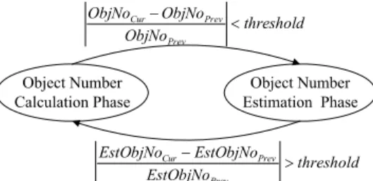
As shown in Fig. 12, the proposed algorithm consists of two phases, object number calculation phase and object number estimation phase, and these two phases are activated in turn. The descriptions of these two phases are as follows.
• In object number calculation phase, scheme redundancy removal is used to get the ex-act number of the sensed objects. As mentioned in section 1, all sensors report the iden-tities of all sensed objects, and redundant ideniden-tities will be removed in an in-network manner for power saving.
• In object number estimation phase, scheme SDARIA and algorithm GPE are both used to get the lower bounds, upper bounds and estimations of the sensed objects. Although the resultant lower bounds, upper bounds and estimations are not the exact object num-bers, they are still able to give users some information about the exact object numbers.
Object Number Calculation Phase Object Number Estimation Phase threshold ObjNo ObjNo ObjNo Prev Prev Cur− < threshold EstObjNo EstObjNo EstObjNo Prev Prev Cur− >
Fig. 12. The phase transition diagram of the proposed two-phase algorithm.
The phase transition conditions are as follows. Let ObjNoCur and ObjNoPrev be the
exact object numbers in, respectively, current and previous calculations in object number calculation phase. We also let EstObjNoCur and EstObjNoPrev be the estimated object
numbers in, respectively, current and previous estimations in object number estimation phase. The system administrators have to specified a parameter threshold where 0 <
threshold < 1. The algorithm will step from object number estimation phase into object
number calculation phase when
. Cur Prev Prev EstObjNo EstObjNo threshold EstObjNo − >
In addition, the algorithm will step from object number calculation phase into object number estimation phase when
Cur Prev Prev ObjNo ObjNo threshold ObjNo − <
for a while. When energy-conservation is of high importance, the value of threshold should be set to close to one. Thus, the algorithm will be in object number estimation phase for a long time to reduce energy consumption. On the other hand, when accuracy is of high importance, the value of threshold should be set to close to zero.
By using the proposed algorithm, users can get more information on object numbers than by using scheme GPE and algorithm SDARIA only. In addition, using the proposed algorithm makes the sensors save more power than using scheme redundancy removal.
5. CONCLUSION
In this paper, we addressed the problem of resource inventory applications over wireless sensor networks. To reduce energy consumption, each sensor reports only the number of the sensed object to the server, and the server will estimate the object number according to the received reports of all sensors. In view of this, we designed algorithm GPE to estimate the object numbers. Several experiments were conducted to measure the performance of algorithm GPE. The experimental results showed that with a proper grid size ratio, algorithm GPE was able to obtain close approximations of object numbers in reasonable execution time. In our experiments, the approximations of algorithm GPE
were around 95%-115% of the exact object numbers. This result showed that algorithm GPE is more suitable than prior schemes for practical use.
REFERENCES
1. I. F. Akyildiz, W. Su, Y. Sankarasubramaniam, and E. Cayirci, “A survey on sensor networks,” IEEE Communications Magazine, 2002, pp. 102-114.
2. S. D. Glaser, “Some real-world applications of wireless sensor nodes,” in
Proceed-ings of SPIE Symposium on Smart Structures and Materials, 2004, pp. 344-355.
3. A. Chen, R. R. Muntz, S. Yuen, I. Locher, S. Park, and M. B. Srivastava, “A support infrastructure for the smart kindergarten,” IEEE Pervasive Computing, Vol. 1, 2002, pp. 49-57.
4. J. Hill, R. Szewczyk, A. Woo, S. Hollar, D. Culler, and K. Pister, “System architec-ture directions for network sensors,” in Proceedings of the 9th International
Con-ference on Architectural Support for Programming Languages and Operating Sys-tems, 2000, pp. 93-104.
5. K. Chintalapudi, R. Govindan, G. Sukhatme, and A. Dhariwal, “Ad-hoc localization using ranging and sectoring,” in Proceedings of the IEEE INFOCOM Conference, 2004, pp. 2662-2672.
6. Y. Shang and W. Ruml, “Improved MDS-based localization,” in Proceedings of the
IEEE INFOCOM Conference, 2004, pp. 2640-2651.
7. J. Considine, F. Li, G. Kollios, and J. Byers, “Approximate aggregation techniques for sensor databases,” in Proceedings of the 20th IEEE International Conference on
Data Engineering, 2004, pp. 449-460.
8. C. Intanagonwiwat, D. Estrin, R. Govindan, and J. Heidemann, “Impact of network density on data aggregation in wireless sensor networks,” in Proceedings of the 22nd
IEEE International Conference on Distributed Computing Systems, 2002, pp. 457-458.
9. S. Madden, M. J. Franklin, J. M. Hellerstein, and W. Hong, “TAG: A tiny aggrega-tion service for ad hoc sensor networks,” in Proceedings of the 5th Symposium on
Operating Systems Design and Implementation, 2002, pp. 131-146.
10. G. Simon, M. Maroti, A. Ledeczi, G. Balogh, B. Kusy, A. Nadas, G. Pap, J. Sallai, and K. Frampton, “Sensor network-based countersniper system,” in Proceedings of
the 2nd ACM International Conference on Embedded Networked Sensor Systems,
2004, pp. 1-12.
11. N. Xu, S. Rangwala, K. K. Chintalapudi, D. Ganesan, A. Broad, R. Govindan, and D. Estrin, “A wireless sensor network for structural monitoring,” in Proceedings of the
2nd ACM International Conference on Embedded Networked Sensor Systems, 2004,
pp. 13-24.
12. N. Heo and P. K. Varshney, “Energy-efficient deployment of intelligent mobile Sen-sor networks,” IEEE Transactions on System, Man, and Cybernetics − Part A:
Sys-tems and Humans, Vol. 35, 2005, pp. 78-92.
13. A. Rogers, E. David, and N. R. Jennings, “Self-organized routing for wireless mi-crosensor networks,” IEEE Transactions on System, Man, and Cybernetics − Part A:
Systems and Humans, Vol. 35, 2005.
commu-nication protocol for wireless microsensor networks,” in Proceedings of the 33rd
Hawaii International Conference on System Sciences, 2000.
15. T. H. Lin and P. Huang, “Sensor data aggregation for resource inventory applica-tions,” in Proceedings of the IEEE Wireless Communications and Networking
Con-ference, 2005, pp. 2369-2374.
16. D. M. Doolin, S. D. Glaser, and N. Sitar, “Software architecture for GPS-enabled wildfire sensorboard,” TinyOS Technology Exchange, 2004.
17. V. Dahllof and P. Jonsson, “An algorithm for counting maximum weighted inde-pendent sets and its applications,” in Proceedings of the 13th Annual ACM/SIAM
Symposium on Discrete Algorithms, 2002, pp. 292-298.
18. Y. Theodoridis, J. R. O. Silva, and M. A. Nascimento, “On the generation of spatial-temporal datasets,” in Proceedings of the 6th International Symposium on Large
Spatial Databases, 1999, pp. 147-164.
19. The R-Tree Portal, http://www.rtreeportal.org/.
Jiun-Long Huang (黃俊龍) received his B.S. and M.S. de-grees in Computer Science and Information Engineering De-partment in National Chiao Tung University in 1997 and 1999, respectively, and his Ph.D. degree in Electrical Engineering De-partment in National Taiwan University in 2003. Currently, he is an assistant professor in Computer Science Department in Na-tional Chiao Tung University. His research interests include: mo-bile computing, wireless networks and data mining.
Shih-Chuan Chiu (邱士銓) received the B.S. degree in Computer Science and Information Engineering from Tamkang University and the M.S. degree in Computer Science from Na-tional Chengchi University, in 2002 and 2004, respectively. He is currently working towards the Ph.D. degree in the Department of Computer Science at National Chiao Tung University. His current research interests include data mining, computer music and mo-bile computing.
Xin-Mao Huang (黃信貿) received his M.S. and Ph.D. de-gree from the Electrical Engineering Department of National Taiwan University, Taipei, Taiwan, R.O.C., in 1998 and 2005, respectively. Currently, he is an assistant professor in Computer Science and Information Engineering in Aletheia University. His research interests include data mining, distributed system, and multimedia applications.