國立臺灣大學電機資訊學院電子工程學研究所 碩士論文
Graduate Institute of Electronics Engineering College of Electrical Engineering and Computer Science
National Taiwan University Master Thesis
利用可調整內插法計算邏輯無關項
Don’t-Care Computation via Adjustable Interpolation
陳一心 I-Hsin Chen
指導教授:江介宏 博士 Advisor: Jie-Hong Jiang, Ph.D.
中華民國 98 年 6 月 June, 2009
Acknowledgements
First, I would like to thank my advisor, Dr. Jie-Hong Roland Jiang. Without his patience and enthusiasm for students, I could not learn so much about academic study and theoretical research. He never hesitates to give his students valuable advice and helpful direction. From him, I saw what an esteemed teacher is.
Second, I would like to thank all the members in ALCom Lab. For Hong-Yuan Lin, Chung-Min Li, Wei-Lun Hung, Wei-Chieh Wang, and Sz-Cheng Huang, we had delighted period in the building EE-II. For Hsuan-Po Lin and Ruei-Rung Lee, we had memorable time both in study and life. Also, Chih-Fan Lai, Fu-Rong Wu, Meng-Yan Li, Jane-Chi Lin, and Chia-Chao Kan, are excellent companions and friends. Without them, I could not have such grateful and wonderful experience in these years.
Especially, I would like to thank all the other friends who stood with me, no matter in the cheerful hours or the difficult moments.
Finally, I would like to thank my parents, my sister, and my girl friend. For the every step in my life, they are always fully behind me and support me, thank you.
To them, I dedicate this thesis.
I-Hsin Chen
National Taiwan University June 2009
摘要
近年來在邏輯合成與驗證的領域中,內插法的應用與日俱增,相關範疇包括 函數相依、二元分解、亞氏分解等。本研究係利用內插法針對多層次電路之節點 計算邏輯無關項。
傳統上,內插可藉由可滿足性問題求解器產生之反證求得,並可利用改寫反 證之結構對內插大小進行調整。但我們在研究過程發現,大部分狀況中,調整可 滿足性問題求解器產生反證後所求得之內插並無太大的改變,內插法的效能因而 受限。
本論文中,我們提出利用可滿足性問題求解之演算法來計算邏輯無關項,並 發展出一套針對可滿足性問題求解器改變內插大小的技巧,包括調整初始變數優 先序及改變布林初始值,同時利用電路結構簡化問題模型以加快求解速度。實驗 結果顯示,該改變內插大小的方法讓求解邏輯無關項之演算法在可接受的時間 內,較未使用該方法時求出更多的邏輯無關項。
關鍵詞:內插法、邏輯網路、邏輯無關項、可滿足性問題求解、可調整內插
Abstract
In recent years, there have been a variety of applications of interpolation in logic synthesis and verification, such as functional dependency, bi-decomposition, and Ashenhurst decomposition. The goal of this research is to compute don’t-cares for a given node in a multi-level network by using interpolation.
Traditionally, an interpolant can be derived from a refutation proof given by a SAT solver, and its onset can be adjusted via rewriting the structure of the refutation proof.
However, in most cases, the interpolant derived by the refutation proof generated by a SAT solver can not be adjusted too much. As a result, the application of interpolation is limited.
In this thesis, we propose SAT-based don’t-care computation algorithms via interpolation. In addition, a set of techniques has been developed for a SAT solver to adjust the solution space of the interpolant. The methods include setting the initial variable activities and altering the Boolean initial values. The circuit structure has also been utilized to simplify the problem to accelerate SAT solving. Experiments show that the algorithms can get more don’t-cares while applying the interpolation sizing method to the algorithms.
Keywords: Craig interpolation, logic network, don’t-care, SAT solving, adjustable interpolant
Contents
Acknowledgements ...i
摘要... ii
Abstract... iii
Contents...iv
List of Figures...vi
List of Tables ... viii
Chapter 1 Introduction...1
1.1 The Origin of Don’t-Cares...1
1.2 Previous Work...3
1.3 Our Contributions ...5
1.4 Organization of the Thesis...6
Chapter 2 Preliminaries ...7
2.1 Boolean Network and Function...7
2.2 Satisfiability Problem and Solver ...8
2.3 Resolution and Refutation Proof ...9
2.4 Craig Interpolation Theorem ...10
2.4.1 Interpolant Strengthen ...12
2.5 Circuit to CNF Conversion...14
Chapter 3 Don’t-Care Computation Algorithms ...15
3.1 CDC Computation Method 1 (CDCC1) ...16
3.2 CDC Computation Method 2 (CDCC2) ...18
3.3 CNF Simplification...20
3.4 Adjustable Interpolation ...21
3.4.1 Swap Rules...21
3.4.2 Initial Variable Activities...26
3.4.3 Boolean Initial Values ...28
3.5 Verification ...28
3.5.1 Combinational Equivalence Checking...28
3.5.2 Absorbing Checking...29
Chapter 4 Experimental Results ...30
4.1 Variable Decision Order ...30
4.2 Adjustable Interpolation on CDCC1 ...33
4.3 Adjustable Interpolation on CDCC2 ...40
Chapter 5 Conclusions and Future Work...46
Bibliography ...47
List of Figures
Figure 1.1: An example of SDCs and ODCs...2
Figure 1.2: Mishchenko proposed the miter charactering the care-set...4
Figure 2.1: A Boolean network and the corresponding DAG. ...7
Figure 2.2: There are three clauses, four variable, and six literals in the CNF...8
Figure 2.3: The interpolant P is an approximation of A, and disjoints B. ...10
Figure 2.4: The ITP computation...11
Figure 2.5: The mapping of refutation proof and the interpolant...12
Figure 2.6: There could be more than one interpolant in different strength...12
Figure 2.7: Two swap rules used to adjust the interpolant. ...13
Figure 2.8: An AND gate transfers to a CNF representation...14
Figure 3.1: Example of SDCs and ODCs...15
Figure 3.2: The miter of CDCC1 algorithm. ...16
Figure 3.3: Algorithm of method 1...17
Figure 3.4: The miter of CDCC2 algorithm. ...18
Figure 3.5: Algorithm of CDCC2...19
Figure 3.6: The illustration of target node, TFO and TFOI...20
Figure 3.7: The nodes in the TFOI area share the same variables...21
Figure 3.8: The relation between (a) swap rule 1 and (b) the corresponding refutation proof structure...22 Figure 3.9: The solution space of (a) original interpolant, if we use rule 1, then (b) a
stronger interpolant can be gotten. ...23
Figure 3.10: The relation between (a) swap rule 2 and (b) the corresponding refutation proof structure...24
Figure 3.11: The illustration of swap rule 1 with multiple fanouts. ...25
Figure 3.12: The illustration of swap rule 2 with multiple fanouts. ...26
Figure 3.13: Decision and learned clause in a refutation proof...27
Figure 3.14: The miter for don’t-care verification...29
Figure 4.1: Original variable count vs. levels in refutation proof in MiniSat. ...31
Figure 4.2: Variable count vs. levels by small variable ID decision first. ...31
Figure 4.3: Variable count vs. levels by large variable ID decision first...32
Figure 4.4: Interpolant on set changing by CDCC1 + M on benchmark ISCAS-85...38
Figure 4.5: Interpolant on set changing by CDCC1 + I + D on benchmark ISCAS-85..38
Figure 4.6: Interpolant on set changing by CDCC1 + M on benchmark ISCAS-89...39
Figure 4.7: Interpolant on set changing by CDCC1 + I + D on benchmark ISCAS-89..39
Figure 4.8: Interpolant on set changing by CDCC2 + M on benchmark ISCAS-85...44
Figure 4.9: Interpolant on set changing by CDCC2 + I + D on benchmark ISCAS-85..44
Figure 4.10: Interpolant ons et changing by CDCC2 + M on benchmark ISCAS-89...45 Figure 4.11: Interpolant on set changing by CDCC2 + I + D on benchmark ISCAS-89.45
List of Tables
Table 4.1: McMillan adjustable method (CDCC1 + M)...34
Table 4.2: Our adjustable method (CDCC1 + I + D). ...34
Table 4.3: McMillan adjustable method (CDCC1 + M)...35
Table 4.4: Our adjustable method (CDCC1 + I + D). ...36
Table 4.5: The optimal ratio of don’t-care computation via adjustable interpolation. ....41
Table 4.6: McMillan adjustable method (CDCC2 + M)...41
Table 4.7: Our adjustable method (CDCC2 + I + D). ...41
Table 4.8: McMillan adjustable method (CDCC2 + M)...42
Table 4.9: Our adjustable method (CDCC2 + I + D). ...43
Chapter 1 Introduction
As the focus of logic synthesis and verification shifted to multi-level networks, computing don’t-cares of a given node in a Boolean network becomes more and more important. Such don’t-care information can be used to provide additional flexibility to simplify a Boolean expression. In addition, using don’t-cares for technology independent logic synthesis of multi-level networks has been a major technique in the area of logic optimization. As a result, efficient methods to compute don’t-cares are necessary for these logic manipulations. In this chapter, we first give the introduction to don’t-cares and exam previous work related to don’t-care computation. We then summarize our contributions, and finally, outline this thesis.
1.1 The Origin of Don’t-Cares
Don’t-cares allow a node in a logic network to have a flexible output value either 0 or 1 under an input assignment. Moreover, such don’t-care conditions are the combinations of external don’t-cares (XDCs), observability don’t-cares (ODCs) and satisfiability don’t-cares (SDCs). External don’t-cares are given by assigning the minterms at the primary input. For instances, the values 1010 through 1111 in binary, or 10 through 15 in decimal, never happen on a binary coded decimal (BCD) [18] function.
Therefore, those values are the external don’t-cares for a function in the binary coded
decimal system.
Unlike external don’t-cares, observability and satisfiability don’t-cares exist due to the multi-level network structures. In other words, the input assignments of an internal node depend on the primary inputs, but not all the combination of assignments can be generated at the internal node. Accordingly, those assignments which never appear at the node form the satisfiability don’t-cares. On the other hand, observability don’t-cares arise under the conditions that the output value of a node does not affect the primary outputs. Hence, they compose the observability don’t-cares. Below we give an example of the satisfiability and observability don’t-cares.
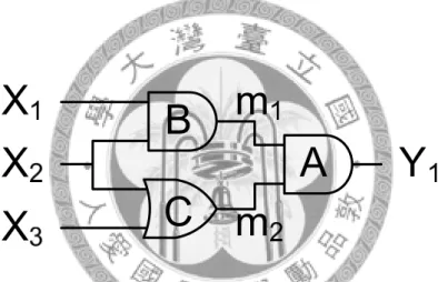
Figure 1.1: An example of SDCs and ODCs.
In Figure 1.1, the node A has a satisfiability don’t-cares with (m1, m2) equal to (1, 0).
For the node A, if we want m1 to be one, this requires X2 to be one. For m2 to be zero, in the other side, this requires X2 to be zero. X2 could not be different values simultaneously. As a consequence, the combination (1, 0) never appears at (m1, m2) and this becomes the satisfiability don’t-care. In addition, the node C has observability don’t-cares in the global space with X1 or X2 equals to zero. While X1 or X2 equals to zero, it leads m1 to be zero. Zero is the controlling values of AND-gate, so Y1 is also zero whatever the value m2 is. As a result, (0, 0) and (0, 1) form the observability
don’t-cares of node C in the global space (X2, X3).
Satisfiability and observability don’t-cares are together called complete don’t-cares (CDCs) [8]. Complete don’t-cares form a superset of the compatible observability don’t-cares (CODCs) [7]. Compatible observability don’t-cares and satisfiability don’t-cares conventionally are the forms used in logic optimization [1]. Furthermore, the amount of don’t-cares computed for complete don’t-cares is larger than for compatible observability don’t-cares. Moreover, substituting a node’s function by a completely specified function compatible with its complete don’t-cares does not change the network’s output. Therefore, complete don’t-cares are important for logic optimization.
1.2 Previous Work
There are some previous efforts which present circuit optimization using the don’t-cares. The strategies of these methods include the image computation via binary decision diagrams (BDDs), quantifier elimination through SAT-based algorithm, and image approximation utilizing clause limited to fixed length. We summarize them as follow.
First, observability don’t-cares are often too large to be efficiently computed in the optimization process. Therefore, Savoj and Brayton [1] used compatible observability don’t-cares (CODCs) instead of observability don’t-cars to avoid the computation on redundant observability don’t-cares.
Second, Savoj and Brayton [2] computed don’t-care information using an image computation approach based on binary decision diagrams. This method computes compatible observability don’t-care sets, which allow simultaneous modification on
multiple nodes. However, it sacrifices the optimization flexibility.
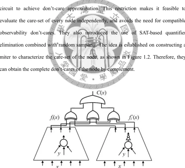
Furthermore, Mishchenko and Brayton [8] proposed the concepts of complete don’t-cares (CDCs), a superset of compatible observability don’t-cares. They showed that the complete don’t-cares computation is comparable to compatible observability don’t-cares in runtime and memory consumption, and the number of don’t-cares is larger than that of compatible observability don’t-cares. The work used Boolean satisfiability solvers instead of binary decision diagrams to avoid the memory explosion problem, which often happens in BDD-based algorithms. They also introduced a windowing technique which restricts the environment to a local subset of the entire circuit to achieve don’t-care approximation. This restriction makes it feasible to evaluate the care-set of every node independently, and avoids the need for compatible observability don’t-cares. They also introduced the use of SAT-based quantifier elimination combined with random sampling. The idea is established on constructing a miter to characterize the care-set of the node, as shown in Figure 1.2. Therefore, they can obtain the complete don’t-cares of the node by complement.
Figure 1.2: Mishchenko proposed the miter charactering the care-set.
Besides, they showed such construction is more robust than the BDD-based
quantifier elimination if the number of node inputs is less than about ten. However, because this method enumerates the minterms of the care-set, it cannot be applied to nodes with a large number of inputs. Our experience suggests that it is not scalable to large-scale circuits without the windowing technique.
McMillan [9] proposed a method of approximate quantifier elimination to compute the strongest over-approximation. This method uses a Boolean satisfiability solver in the machine-learning framework with clauses confined to a given length. The advantage of this approach is that it does not require enumerating the minterms of the care-set. For that reason, it can be applied when the number of node inputs is relatively large. They showed it remains robust in some cases while the BDD-based image computation and minterm enumeration methods fail. However, the restriction of the clause length lost the precision for the computation results.
1.3 Our Contributions
In this thesis, we present two novel algorithms. Different from prior work, our work brings the following distinct features.
- The algorithms are based on SAT solving, but take advantage of the efficiency and scalability of interpolation.
- The computation results of complete don’t-cares can be further enhanced through the adjustable interpolation algorithms.
- This is the first work considering the adjustability of interpolation in the early stage of Boolean satisfiability solving processes.
To summarize, our work is based on the Boolean satisfiability solving. Unlike prior methods, we take advantage of interpolation to enhance the scalability of don’t-care
computation while maintaining efficiency. Further, we propose practical solutions to adjust interpolation to gain better results on don’t-care computation. Our proposed methods including setting initial variable activities and altering the Boolean initial values are useful to modify the solution space of the interpolant. These methods raise the capacity of adjustable interpolation algorithms, and then benefit those algorithms based on interpolation.
1.4 Organization of the Thesis
The rest of the thesis is structured as follows. Chapter 2 provides the required preliminaries and background, including Boolean network and functions, don’t-cares, Boolean satisfiability solving, and Craig interpolation. Chapter 3 describes our don’t-care computation methods and the adjustable interpolation algorithms. Chapter 4 reports the experimental results, and Chapter 5 concludes the thesis and outlines future work.
Chapter 2 Preliminaries
2.1 Boolean Network and Function
A Boolean network or a circuit is a directed acyclic graph (DAG), where nodes correspond to logic gates and directed edges correspond to wire connections between the gates. A node has zero or more fanins. Fanins of a node are other nodes that driving this node. A node has zero or more fanouts. Fanouts of a node are other nodes that driven by this node. The nodes without fanins are called primary inputs (PIs). The nodes without fanouts are called primary outputs (POs). For registers in a sequential circuit, their inputs and outputs are treated as additional POs and PIs. For instance, a Boolean network and its corresponding DAG drawn by ABC [13] are shown in Figure 2.1.
Figure 2.1: A Boolean network and the corresponding DAG.
Boolean function is composed of Boolean variables. A completely Boolean function has the definition as follow.
Definition. A completely specified Boolean function (CSF) is a mapping from
n-dimensional (n≥ Boolean space into a single-dimensional one: 0)
{ }
0,1n →{ }
0,1[8].
If a function with at least one input combination such that the output function is a don’t-care, it is an incompletely specified Boolean function (ISF).
2.2 Satisfiability Problem and Solver
The Boolean satisfiability problem, known as SAT, is determining if there exists a satisfying variable assignment for a given Boolean formula. We begin with required definitions. Let V =
{
v1,...,vk}
be a finite set of Boolean variables. A literal is a variable vi or its negation ¬ . A clause vi c is a disjunction of literals. We assume that all the clauses are non-tautological so that there would never be a variable and its negation in a same clause and produce a true. A SAT instance is a conjunction of clauses, or a conjunctive normal form (CNF). For instance, Figure 2.2 shows a conjunctive normal form with three clauses, four variables, and six literals.(a b c b+ + )( + ¬ ¬ c)( d)
Figure 2.2: There are three clauses, four variable, and six literals in the CNF.
A solver for the Boolean satisfiability problem is called a SAT solver. When solving a problem, a SAT solver assigns Boolean values to those variables in turn if they
were not assigned until a satisfiable instance occurs or the unsatisfiability happens. In some modern SAT solvers, such as MiniSat [11], heuristics such as variable activity are used to choose variable for assigning value. Activity heuristic is a dynamic variable ordering mechanism. Each variable comes with a value called activity, and the activity varies upon the frequency of variable appearing in the conflict clauses.
A SAT solver gives a satisfying assignment when the given clause set is satisfiable, otherwise it is unsatisfiable. Some modern SAT solvers produce a refutation proof when the problem is unsatisfiable. The refutation proof proves the problem is unsatisfiable, and it can be used to generate interpolants.
2.3 Resolution and Refutation Proof
Resolution is a rule of inference leading to a refutation proof. In propositional logic, the resolution rule is a single valid inference rule. It produces a new clause implied by two clauses containing complementary literals. The new clause produced by the resolution rule is called the resolvent of the input clauses. A resolvent of two clauses
c1= ∨v A and c2 = ¬ ∨v B is the clause A B∨ , provided that A B∨ is non-tautological. We call v the pivot variable of c1 and c2. In fact, if there exists a resolvent of c1 and c2, we can write the resolvent as the form∃ ∧(c1 c2).
Then we have the definition of an unsatisfiability refutation proof ∏ . Given the set of clauses C, ∏ is a directed acyclic graph( ,V E∏ ∏), where V∏ is a set of clauses.
For every vertex c V∈ , it must be one of the following conditions: (1)∏ c C∈ ⇒ c is a root, or (2) c has exactly two predecessors, c1 and c2 ⇒ c is the resolvent of c1 and c2, and (3) the empty clause is the unique leaf. Following the refutation proof, we can get the empty clause by resolution rule, and prove the unsatisfiability of the clause set C.
2.4 Craig Interpolation Theorem
We describe the definition of an interpolant. It was proposed by Craig in 1957 [4].
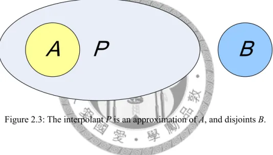
An interpolant for the unsatisfiable pair (A, B) is a formula P with the following three properties:
– A implies P
– P B∧ is unsatisfiable
– P refers only to the common variables of A and B
Figure 2.3: The interpolant P is an approximation of A, and disjoints B.
Figure 2.3 illustrates the concept of interpolant. In fact, we can consider the interpolant as an over-approximation of formula A, while P maintains the feature that disjoints with B. There is an intuition to stats the existence of interpolants. That is, the smallest interplant is∃x Ac( ), where x stands for those variables appear in A but not c appear in B. In the other way, the largest interplant is∀y Bc( ), wherey stands for those c variables appear in B but not appear in A.
Pudlak [14] and Krajiček [15] proposed methods that if given a proof of unsatisfiability of A B∧ , P can be derived in linear time. Multiplexers are used to generator the interpolant. Here we use the method proposed by McMillan in 2005 [5].
We divide the clauses into two sets, namely A and B, and then we obtain the refutation proof ∏ of A B∧ via SAT solving. We say a variable is global if it appears both in A and B, and a variable is local to A if it appears only in A. Here we use g(c) to denote the disjunction of the global literals in a clause c and use l(c) to denote the disjunction of the literals local to A in a clause c.
Let (A, B) be the division of clause sets and ∏ be a refutation proof of its unsatisfiability and the leaf vertex is given FALSE. Let p(c) be a Boolean formula where c is any vertices in V∏, and then ITP-Function is defined in Figure 2.4.
ITP-Function( ) 1 for each v V∈ ∏ 2 do if c is a root 3 then if c A∈
4 then ( )p c ←g c( ) 5 else ( )p c ←TRUE 6 else if v is local to A
7 then p c( )← p c( )1 ∨ p c( )2 8 else p c( )← p c( )1 ∧ p c( )2 Figure 2.4: The ITP computation.
Note that c1 and c2 are two predecessors of c, and v is the pivot variable. Thus the
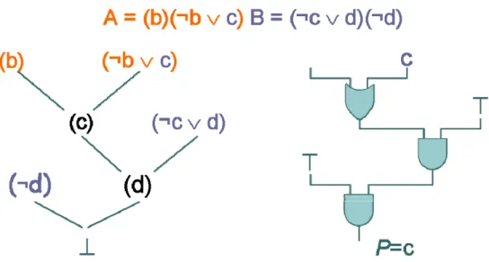
∏ -interpolant of (A, B) is p(FALSE). McMillan gave the detail proof about this method [16]. In the other way, interpolant indeed is a circuit following the structure of the refutation proof. Figure 2.5 gives an example of such interpolant.
Figure 2.5: The mapping of refutation proof and the interpolant.
This approach directs us a way to compute interpolant simply. However, the interpolants derived by this method are usually weak and may not be good enough in practice, especially for our applications in computing don’t-cares.
2.4.1 Interpolant Strengthen
In our algorithms, we need a process to derive different strength interpolants. For example in Figure 2.6, P and P’ are implied by A, and both are unsatisfiable with B, but they have different strength.
Figure 2.6: There could be more than one interpolant in different strength.
In other words, a method to adjust the interpolant to generator interplant with difference strength, or different solution space is necessary.
Jhala and McMillan [3] presented a method to compute strong interpolants. This method is mainly using swap rules to rewrite the refutation proof to derived different strength interpolant.
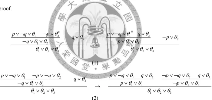
Overall, to strengthen the interpolant, we would better move the local resolutions toward the hypothesis in a refutation proof; meanwhile, the global resolutions go downward to the conclusion. In such way we move the OR gates toward the inputs of the interpolant circuit and the AND gates toward the output, thus we strengthen the interpolant. To achieve this, two rules in Figure 2.7 are applied to rewrite the refutation proof.
1 3
1 2
2 3
1 3
1 2
1 2 3 1 2 3
p q q
p q p
p
q p
q
θ θ
θ θ θ θ
θ θ θ θ
θ θ θ θ θ θ
∨ ¬ ∨ ∨
∨ ¬ ∨ ¬ ∨ ∨ ¬ ∨
∨ ∨
¬ ∨ ∨ →
∨ ∨ ∨ ∨
(1)
1 3 2 3
1 2
3
1 3 2 3
1 2
1 2 3 1 2 3
p q q p q q
p q p q
q p p
q
θ θ θ θ
θ θ θ
θ θ θ θ
θ θ
θ θ θ θ θ θ
∨ ¬ ∨ ∨ ¬ ∨ ¬ ∨ ∨
∨ ¬ ∨ ¬ ∨ ¬ ∨ ∨
∨ ∨ ¬ ∨ ∨
¬ ∨ ∨ →
∨ ∨ ∨ ∨
(2)
Figure 2.7: Two swap rules used to adjust the interpolant.
Applying these two rules throughout the refutation proof structure, we can basically raise the resolutions with local pivot variables to the top of the refutation proof, and the resolutions with global pivot variables to the bottom. But the price is that it may expand the size of the refutation proof exponentially. Instead, Jhala and McMillan adopted a limited approach to keep the size of refutation proof linear.
First, mark all the resolution steps in the refutation proof whose consequent is used as the antecedent in more than one subsequent step. Then, traverse the refutation proof from antecedents to consequents topologically, and apply the rewrite rules on every local atoms q until meet the marked steps or hypothesis. Although this approach do increase the size of the refutation proof every time when the second rewrite rule is applied, the final number of occurrences of a step s is bounded by the number of occurrences of ¬ in the original refutation proof that were resolved by s. As a result, q the number of resolutions we obtain after raising all the resolutions on local atoms is linear in the size of the original refutation proof, so as the interpolant. However, our experiments show that such method has its limitation. In Section 3.4, we explore the reason and present our heuristic to achieve effective adjustable interpolation.
2.5 Circuit to CNF Conversion
Given a circuit netlist, it can be converted to a CNF formula by a way preserving the satisfiability. The conversion is achievable in linear time by introducing extra intermediate variables [10]. In the consequence, we shall assume that the clause set of a Boolean formula is available from such conversion. Figure 2.8 shows the transformation of an AND gate to a CNF representation.
( )
( )( )
( ( ))( ( ) )
( )( )( )
c ab
c ab
c ab ab c
c ab ab c
c a c b a b c
=
⇒ ↔
⇒ → →
⇒ ¬ + ¬ +
⇒ ¬ + ¬ + ¬ + ¬ +
Figure 2.8: An AND gate transfers to a CNF representation.
Chapter 3
Don’t-Care Computation Algorithms
This chapter presents two novel algorithms based on interpolation to compute complete don’t-cares (CDCs). We fast review that complete don’t-cares consist of satisfiability don’t-cares and observability don’t-cares. Satisfiability don’t-cares are terms that never appear at the inputs of a node, and observability don’t-cares are terms for which changes to a node’s inputs are not observable in the primary outputs. Figure 3.1 shows an example where (x, y) equals (0, 1) of F is a satisfiability don’t-care, and all input assignments of G are observability don’t-cares if (a, b) equals to (1, 1).
Figure 3.1: Example of SDCs and ODCs.
Traditional way to compute complete don’t-cares usually involves image computation. The process of image computation is often slow. In this chapter, we introduce the algorithms using interpolation to compute complete don’t-cares.
3.1 CDC Computation Method 1 (CDCC1)
As introduced in Chapter 2, interpolant of (A, B) is an over-approximation of set A.
Therefore, if an over-approximate care-set is available, an under-approximate complete don’t-cares can be derived by complement.
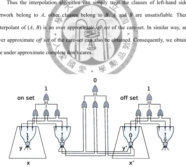
The strategy of method 1 is to construct a miter that characterizes the on set of the care-set, as the left-hand side shown in Figure 3.2. On the other hand, another miter is constructed to characterize the off set of the care-set, as the right-hand side shown in Figure 3.2. Since the on set and off set of the care-set are disjoint to each other, the final network shown in Figure 3.2 must be unsatisfiable.
Thus the interpolation algorithm can simply treat the clauses of left-hand side network belong to A, other clauses belong to B. A and B are unsatisfiable. Then interpolant of (A, B) is an over approximate on set of the care-set. In similar way, an over approximate off set of the care-set can also be obtained. Consequently, we obtain the under approximate complete don’t-cares.
Figure 3.2: The miter of CDCC1 algorithm.
Note that if only basic interpolant is used, the computed on set and off set of the care-set could be complement to each other, and the computed complete don’t-cares are empty. Therefore, CDCC1 requires a process to derive different strength interpolants.
We introduce the rewrite rules and our proposed methods to get strong interpolants in Section 3.4. Finally, Figure 3.3 summarizes the algorithm of CDCC1.
CDC Computation Method 1 ( )
1. Construct the network
2. A
←clauses of left-hand side network 3. B
←other clauses in the network 4. onset
←interpolant of (A, B)
5. A’
←clauses of right-hand side network 6. B’
←other clauses in the network
7. offset
←interpolant of (A’, B’) 8. return ( onset ∪ offset )
Figure 3.3: Algorithm of method 1.
3.2 CDC Computation Method 2 (CDCC2)
The CDCC1 proposed in previous section runs in good speed, however, the experiments do not show promising results. The amount of computed don’t-cares is less.
Hence, we developed the other similar algorithm, and we call it the CDCC2.
Our strategy in CDCC2 is similar to that in CDCC1. First, we construct a miter that characterizes the care-set followed by a miter that characterizes don’t-care set and probably some overlap with care-set. Figure 3.4 shows the final network.
Figure 3.4: The miter of CDCC2 algorithm.
In Figure 3.4, X is global care-set, and X’ is global don’t-care set. Although x and x’ are different, but they could generate the same value at y and y’. As a result, the overlapping occurs. Since the left-hand side network may overlap the right-hand side network in y. the whole network may be satisfiable. To make use of the interpolation algorithm, the overlap part must be excluded. This can be simply done by iteratively adding the overlap instances as conflict clauses to the solver. In practice, the overlap
part rarely happens, thus this process can be done efficiently.
As soon as the miter is unsatisfiable, the interpolation algorithm can treat the clauses of the left-hand side network belong to A, other clauses belong to B. Then we get the interpolant of (A, B) as an approximate care-set. As a result, approximate complete don’t-cares can be obtained.
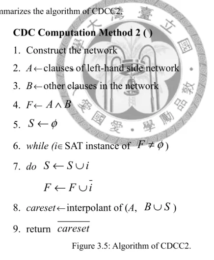
Note that in the process of overlap instances exclusion, some don’t-care set instances are excluded from the network, thus the approximate care-set obtained by interpolation algorithm could be an over-approximation of the exact care-set. Thus completed don’t-cares obtained by CDCC2 could be an under-approximation. Figure 3.5 summarizes the algorithm of CDCC2.
CDC Computation Method 2 ( )
1. Construct the network
2. A
←clauses of left-hand side network 3. B
←other clauses in the network 4. F
←A B ∧
5. S ← φ
6. while (i
∈SAT instance of F ≠ φ ) 7. do S ← ∪ S i
F ← ∪ F i
8. careset
←interpolant of (A, B ∪ S ) 9. return careset
Figure 3.5: Algorithm of CDCC2.
To summarize, CDCC1 needs two SAT solving and interpolation, and CDCC2 may need to run SAT solving several times.
3.3 CNF Simplification
The time needed to solve a Boolean satisfiability problem depends on the complexity of the problem. It has been shown that minimizing the size of the CNF representation and removing unnecessary variables effectively improve SAT run time [12]. We utilize the symmetric structure of the miter to simplify the CNF representation in our algorithms. When constructing the CNF representation, we do following two rules, elimination and sharing variable to minimize the CNF representation.
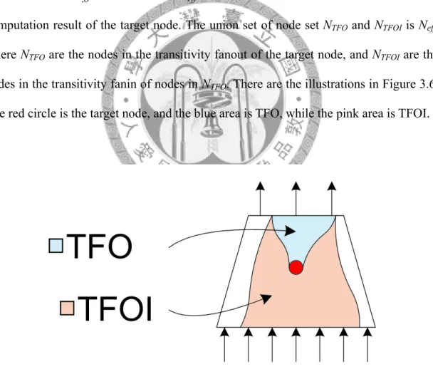
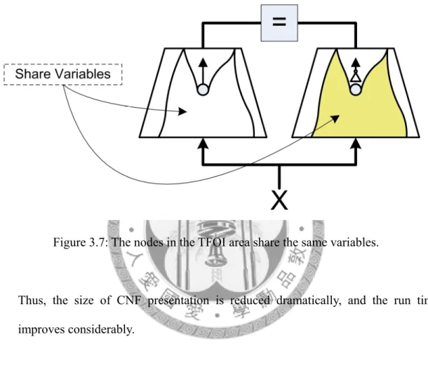
First we define some terms. Target node is the node which we compute the don’t-cares. The effective node set Neff is a set of nodes that affect the don’t-care computation result of the target node. The union set of node set NTFO and NTFOI is Neff, where NTFO are the nodes in the transitivity fanout of the target node, and NTFOI are the nodes in the transitivity fanin of nodes in NTFO. There are the illustrations in Figure 3.6.
The red circle is the target node, and the blue area is TFO, while the pink area is TFOI.
Figure 3.6: The illustration of target node, TFO and TFOI.
– Elimination: We eliminate those nodes not in Neff from CNF representation,
– Sharing variable: For the nodes in Neff but not in NTFO, they share variables with the repeat part in the miter.
For the nodes not in effective network Neff, that is, the nodes in the white area in the Figure 3.6 are dropped from the CNF representation.
Figure 3.7: The nodes in the TFOI area share the same variables.
Thus, the size of CNF presentation is reduced dramatically, and the run time improves considerably.
3.4 Adjustable Interpolation
In Chapter 2, we described the fundamental of interpolation and the theorem to strengthen the interpolant. Here we present the techniques used for computing strong interpolants obtained from a refutation proof in this thesis.
3.4.1 Swap Rules
As McMillan mentioned [3], we can use rule (1) and rule (2) in Figure 2.7 to
strengthen the interpolant. We give the detail descriptions here. For the clarity, we re-express the rule 1 with the same notation used here in Figure 3.8 (a).
2 3
1 2
1 3
2 3
1 2
1 2 3 1 2 3
g l l
g l
l g
g l
θ θ
θ θ θ θ
θ θ θ θ
θ θ θ θ θ θ
∨ ∨ ¬ ∨
¬ ∨ ∨ ∨ ¬ ∨ ¬ ∨
∨ ∨
∨ ∨ →
∨ ∨ ∨ ∨
g
(a)
1 2
4 3
5
﹁g+θ1 g+l+θ2
﹁l+θ3 g
l l+θ1+θ2
θ1+θ2+θ3
3 2
4' 1
5
﹁l+θ3 g+l+θ2
﹁g+θ1
l
g
g+θ2+θ3
θ1+θ2+θ3 Rule 1
(b)
Figure 3.8: The relation between (a) swap rule 1 and (b) the corresponding refutation proof structure.
Figure 3.8 (b) is a direct acyclic graph representing a part of a refutation proof. The nodes represent the clauses which could be a root or a resolvent. Under each node, a CNF represents the content of the resolvent. The orange word represents the pivot variable used to derive the resolvent. One should be noticed that the node 4 is destroyed after swapping. A new node 4’ replaces the original node with different resolvent.
M N K
MN + K
(a)
(b)
M N K
MN + MK
Figure 3.9: The solution space of (a) original interpolant, if we use rule 1, then (b) a stronger interpolant can be gotten.
Figure 3.9 shows the effect of rule 1. The circuit in Figure 3.9 (a) is the original interpolant derived by the refutation proof structure of the left part in Figure 3.8, assume the function corresponding to node 1 is M, and node 2 is N, and node 3 is K. The resolvent resolving on global variable is replaced with an AND-gate; the one resolving on local variable is replaced by an OR-gate. As a result, the function of the interpolant is MN + K. The minterm number of the space is six, for the (M, N, K) pair equals to (110), (111), (001), (011), (101), and (111). In the other way, the interpolant in Figure 3.9 (b) is MN + MK, the corresponding minterms are (110), (101), and (111). Thus, after applying the rule 1, the solution space of the interpolant shrinks from six to three.
For the clarity, we also re-expressed rule 2 and the corresponding refutation proof structure in Figure 3.10.
1 3 2 3
1 2
3
1 3 2 3
1 2
1 2 3 1 2 3
g l l g l l
g l g l
l g g
l
θ θ θ θ
θ θ θ
θ θ θ θ
θ θ
θ θ θ θ θ θ
¬ ∨ ∨ ¬ ∨ ∨ ∨ ¬ ∨
¬ ∨ ∨ ∨ ∨ ¬ ∨
¬ ∨ ∨ ∨ ∨
∨ ∨ →
∨ ∨ ∨ ∨
(a)
(b)
Figure 3.10: The relation between (a) swap rule 2 and (b) the corresponding refutation proof structure.
Figure 3.10 (b) is a direct acyclic graph representing a part of a refutation proof.
Different from rule 1, rule 2 is used when the node 1 and node 2 have the same local variable l simultaneously. At the process of raising a local variable, an extra node need to be generator in order to ensure the resolvent remain the same at node 5. Also, node 4 is destroyed and new node 4’ and node 4’’ are generated.
A problem occurs if the resolvent of the original node 4 were used in other resolution step. In other words, the node 4 is a multiple fanout node. When encountering multiple fanout in the refutation proof, McMillan adopts a method that marking the multiple fanout nodes and skipping those marked nodes. By such strategy, they avoid
the possible exponential expansion of the refutation proof size but sacrifice the interpolation adjustability.
In our cases, we proposed a different way. We partial duplicate the structure of multiple fanout nodes. We copy only the parent nodes of the multiple fanout nodes in the refutation proof. In Figure 3.11, we preserve the original node 4 in the new structure, and keep the connection to the other nodes.
1
1 2
3
5
﹁g+θ1 g+l+θ2
﹁l+θ3 g
l θ1+θ2+θ3
3 2
4' 4
5
﹁l+θ3 g+l+θ2
l+θ1+θ2
l
g
g+θ2+θ3
θ1+θ2+θ3 Rule 1
4 l+θ1+θ2
Multiple-Fanout!
﹁g+θ1 g
Figure 3.11: The illustration of swap rule 1 with multiple fanouts.
For the rule 2, the same thought is adopted. Figure 3.12 describes the swapping for the multiple output case for rule 2.
Thus, for single output node in rule 1, no new node will be added. For single output node in rule 2, one new node will be added. For the multiple output cases, rule 1 and rule 2 increase one and two new nodes, respectively.
Figure 3.12: The illustration of swap rule 2 with multiple fanouts.
However, the two rules both fail if the global pivot variable appears in the node 3.
The failure arises because the appearance of global variable changes the resolvent content of the node 5. As a consequence, the different content destroys the refutation proof correctness. This condition happens often and largely decreases the effect of strengthening interpolants.
3.4.2 Initial Variable Activities
We known the way to strengthen the interpolant is letting local variable appears early in the refutation proof. From previous section, it shows difficulty to adjust the interpolant via rewriting the refutation proof because the rules fail often. Instead of rewriting the refutation proof already generated, we propose a heuristic algorithm to affect the Boolean satisfiability solver to produce a good refutation proof in advance.
As introduced, MiniSat, the modern SAT solver, makes decision by considering variable activity heuristics. In the other way, if a variable were decided earlier in the process of SAT solving, it appears later in the refutation proof. This can be shown from
the production of the conflict clauses [17]. Figure 3.13 give an explanation. For the conjunction normal form (a b a+ )( + ¬ ¬ +b)( a b)(¬ + ¬ , if we make decision on a b) variable a by assigning it to be 0, then we produce clauses ( )(b ¬ and generate an b) unsatisfiability. Thus we learn a conflict clause ( )a , which means assigning a to be 0 produces an unsatisfiability. However, the production of this conflict clause in the refutation proof is derived by resolving on the pivot variable b, and the resolution on variable a appears later than b. As a result, if the variable is decided earlier, it resolves later.
Figure 3.13: Decision and learned clause in a refutation proof.
Thus, by controlling the variable activities in the MiniSat, somehow we affect the variable appearing in the refutation proof in proper order. At the beginning, we changed the decay ratio of local variable in MiniSat, but the results were not good. Hence, we decided to set higher initial variable activities for the local variable before the SAT solving starts. We found that this heuristic worked effective and had good results.
3.4.3 Boolean Initial Values
We have known that affecting the Boolean satisfiability problem solver by proper ways help produce better refutation proof. The structure of the refutation proof depends on the internal procedures of the SAT solver, such as decision order and Boolean constraint propagation. Thus, we try to change the Boolean value when a decision is made. In MiniSat, the decision of a variable always is false then true. We change the decision order by trying true first then false. An interesting thing is that this heuristic dose work. The detail research and the reason why will be our future work. It is sure that different decision generates different implication graph, and somehow this strategy help the SAT solver generate better refutation proof.
3.5 Verification
The derived don’t-cares appear as a form of Boolean function with a single primary output. Where the inputs are the node fanins and the only output is one when the input combinations are the don’t-care sets of the node. For such don’t-cares form, we propose a method to verify its correctness.
3.5.1 Combinational Equivalence Checking
When getting the circuit representing the don’t-care terms, we do formal verification on the don’t-care terms to make sure the result is correct. Our method is to construct a miter to check the correctness of don’t-cares. The first part of the miter is the original circuit. The second part of the miter is the modified circuit where the target node is replaced by an exclusive OR gate. The two fanins of the exclusive OR gate are the target node and the primary output of the don’t-care circuit. The miter is shown in
Figure 3.14. When the input of the node is a don’t-care, the output of the don’t-care circuit is 1. Further, the exclusive OR gate inverts the original node output. This makes the two circuits have different value on the target node. If they are equivalence, the input of the node must be a don’t-care, and the correctness of the don’t-care circuit is proved.
Figure 3.14: The miter for don’t-care verification.
3.5.2 Absorbing Checking
Another way we call absorbing checking. After we checked the don’t-care correctness by combinational equivalence checking, we get the correct don’t-care libraries. After that, each time when we need to check our computation results, we just check if the circuit is absorbed by the don’t-care library. This reduces the verification process.
Chapter 4
Experimental Results
Our experiments were implemented using C++ in ABC, a system for sequential synthesis and verification [13]. The proof-logging version of MiniSat was used as the underlying solver [11]. All experiments were performed on a workstation with Xeon 3.4GHz CPUs and 6 GB RAM. The benchmark circuits were ISCAS 85 and ISCAS 89.
4.1 Variable Decision Order
A preliminary experiment targets for discussing the relation between variable decision order and the resolution order, as mentioned in Section 3.4.2. Five CNFs were chosen as the benchmarks. In the following figures, each line represents the variable counts in the corresponding level. For the refutation proofs have different number of levels, we normalized the number of levels from one to ten. When no extra constraints were set, as shown in Figure 4.1, there is no trend of the variable counts in the refutation proof levels. However, in Figure 4.2, we let variables with small ID have higher priority when solver makes the decision. We found those variables appear more frequently in the higher level, as our expectation. In contrast, variables with large ID rise in the lower level. In Figure 4.3, we did the reverse setting for the variables, and the situation of variable counts was opposite to those in Figure 4.2. Variables with small id are decided later, and the result shows they appear in the early levels, as our expectation.
Figure 4.1: Original variable count vs. levels in refutation proof in MiniSat.
Figure 4.2: Variable count vs. levels by small variable ID decision first.
Figure 4.3: Variable count vs. levels by large variable ID decision first.
4.2 Adjustable Interpolation on CDCC1
The experiments are designed to show following features via the don’t-care computation algorithm.
1. The scalability and capability of interpolation algorithm.
2. The efficiency of our methods to adjust the interpolation.
For each don’t-care computation algorithm, we ran two different settings, the algorithm combined with McMillan’s rewriting rules (CDCC + M), and the one combined with our sizing algorithms (CDCC + I + D), both results are compared with the basic algorithm (CDCC) without using the interpolant sizing algorithms. The don’t-care computation algorithms are designed for an arbitrary node in networks. For each network, we reported the average runtime and memory usage per node, and recorded the maximum value of each term among all the nodes. We also set a fifteen seconds time out for the Boolean satisfiability solver.
First, we present the results of CDCC1 algorithm on benchmark ISCAS-85 and ISCAS-89.
Table 4.1 shows the results of the basic CDCC1 algorithm without applying any sizing interpolant method. In the title of the tables, “M” stands for the McMillan’s swap rules, and “I” represents our initial variable activity heuristic, while “D” describes as our decision value heuristic.
Table 4.1: McMillan’s adjustable method (CDCC1 + M).
Time Mem(Mb) Time Mem(Mb)
C17 6 0.05 7.94 0.16 7.94
C432 160 0.04 8.93 0.20 8.96
C499 202 0.05 9.16 0.20 9.18
C880 383 0.04 9.46 0.22 9.52
C1355 546 0.06 10.47 0.26 10.51
C1908 880 0.09 11.32 0.17 11.62
C2670 1253 0.09 12.62 0.19 12.74
C3540 1669 0.17 14.31 0.31 14.42
C5315 2297 0.10 16.35 0.39 16.79
C6288 2416 0.32 17.76 0.58 18.23
C7552 3510 0.16 21.84 0.66 22.14
0.11 12.74 0.30 12.91
Maximum
Average
Name #Node Average
Table 4.2: Our adjustable method (CDCC1 + I + D).
Time Mem(Mb) Time Mem(Mb)
C17 6 0.02 7.81 0.03 7.94
C432 160 0.04 8.92 0.09 8.97
C499 202 0.05 9.16 0.07 9.20
C880 383 0.04 9.46 0.07 9.55
C1355 546 0.06 10.50 0.11 10.59
C1908 880 0.10 11.39 0.17 11.71
C2670 1253 0.10 12.63 0.20 12.96
C3540 1669 0.18 14.31 0.31 14.62
C5315 2297 0.10 16.36 0.39 16.89
C6288 2416 0.32 17.77 0.58 18.28
C7552 3510 0.18 21.84 0.67 22.04
0.11 12.74 0.24 12.98
Maximum
Average
Name #Node Average
Table 4.3: McMillan’s adjustable method (CDCC1 + M).
Time Mem(Mb) Time Mem(Mb)
s27 10 0.02 7.86 0.02 7.93
s208 104 0.02 8.26 0.03 8.38
s298 119 0.02 8.37 0.03 8.48
s344 160 0.03 8.35 0.05 8.74
s349 161 0.03 8.44 0.05 8.65
s382 158 0.03 8.75 0.05 8.80
s386 159 0.03 8.63 0.06 8.95
s400 162 0.03 8.58 0.06 8.84
s420.1 218 0.03 8.56 0.05 8.74
s444 181 0.03 8.84 0.06 8.87
s499 152 0.03 8.91 0.07 9.14
s510 211 0.03 8.72 0.07 8.99
s526 193 0.03 8.50 0.06 8.69
s526n 194 0.03 8.50 0.06 8.67
s635 286 0.04 9.43 0.08 9.77
s641 380 0.04 9.63 0.09 9.74
s713 393 0.04 9.76 0.11 9.91
s820 289 0.03 9.26 0.08 9.95
s832 287 0.03 9.30 0.09 9.82
s838.1 446 0.04 9.43 0.08 9.61
s938 446 0.03 9.34 0.08 9.60
s953 395 0.03 9.68 0.07 9.91
s967 394 0.03 9.61 0.07 9.91
s991 519 0.05 10.29 0.14 10.92
s1196 529 0.05 10.14 0.12 10.25
s1238 508 0.05 9.91 0.12 10.27
s1269 569 0.06 10.15 0.14 10.83
s1423 657 0.05 10.90 0.15 11.07
s1488 653 0.03 10.35 0.08 11.26
s1494 647 0.03 11.00 0.08 11.21
s1512 780 0.03 10.98 0.08 11.76
s3271 1573 0.03 11.51 0.06 11.96
s3330 1789 0.04 13.37 0.14 14.13
s3384 1702 0.04 12.36 0.09 12.57
s4863 2374 0.08 14.51 0.22 15.06
s5378 2794 0.06 15.52 0.17 15.52
s6669 3148 0.11 15.86 0.26 16.92
s9234.1 5597 0.11 23.59 0.69 24.98
s13207 8027 0.09 25.90 0.39 27.24
s15850 9786 0.12 33.35 0.63 36.27
s35932 16065 0.13 38.81 0.48 42.39
s38417 22397 0.20 48.02 0.62 52.77
s38584 19407 0.20 59.41 2.49 76.11
0.05 13.97 0.20 14.97
Average
#Node Average Maximum
Name
Table 4.4: Our adjustable method (CDCC1 + I + D).
Time Mem(Mb) Time Mem(Mb)
s27 10 0.01 7.86 0.02 7.93
s208 104 0.02 8.27 0.02 8.38
s298 119 0.02 8.37 0.03 8.48
s344 160 0.03 8.35 0.05 8.68
s349 161 0.03 8.44 0.05 8.66
s382 158 0.03 8.75 0.05 8.84
s386 159 0.03 8.63 0.07 8.95
s400 162 0.03 8.58 0.06 8.87
s420.1 218 0.03 8.58 0.05 8.76
s444 181 0.03 8.84 0.06 8.90
s499 152 0.03 8.92 0.06 9.16
s510 211 0.03 8.72 0.06 9.02
s526 193 0.03 8.50 0.06 8.72
s526n 194 0.03 8.50 0.05 8.70
s635 286 0.04 9.44 0.09 9.79
s641 380 0.04 9.63 0.11 9.76
s713 393 0.05 9.76 0.11 9.96
s820 289 0.03 9.27 0.08 10.00
s832 287 0.03 9.30 0.09 9.86
s838.1 446 0.04 9.43 0.08 9.72
s938 446 0.04 9.35 0.09 9.73
s953 395 0.03 9.69 0.07 9.91
s967 394 0.03 9.61 0.09 9.91
s991 519 0.05 10.31 0.14 10.96
s1196 529 0.05 10.15 0.12 10.35
s1238 508 0.05 9.92 0.12 10.35
s1269 569 0.06 10.16 0.14 10.91
s1423 657 0.05 10.90 0.16 11.20
s1488 653 0.03 10.36 0.08 11.32
s1494 647 0.03 11.00 0.08 11.28
s1512 780 0.04 10.99 0.08 11.57
s3271 1573 0.04 11.52 0.07 12.06
s3330 1789 0.05 13.37 0.14 14.56
s3384 1702 0.05 12.37 0.10 13.07
s4863 2374 0.09 14.52 0.18 15.11
s5378 2794 0.07 15.52 0.21 15.98
s6669 3148 0.12 15.87 0.28 16.92
s9234.1 5597 0.13 23.60 0.72 25.46
s13207 8027 0.12 25.90 0.56 28.92
s15850 9786 0.17 33.37 0.66 37.50
s35932 16065 0.22 38.82 0.53 42.39
s38417 22397 0.32 48.03 0.75 54.18
s38584 19407 0.30 59.42 2.54 79.65
0.06 13.97 0.21 15.22
Average
#Node Average Maximum
Name
Table 4.1 and Table 4.2 show that for the ISCAS-85 benchmark, most of the nodes can be conquered within 0.5 second and the average memory usage is within 13 Mb.
Table 4.3 and Table 4.4 show that for the ISCAS-89 benchmark, most of the nodes can be conquered within 1 second and the average memory usage is within 15 Mb. The short runtime shows the efficiency of the interpolation algorithms.
We compared the effect of adjustable interpolation by evaluating the solution space of don’t-cares. From Figure 4.4 to Figure 4.7, the value is a normalized don’t-care minterm number which ranges from 0 to 1. While 1 means the don’t-care computed at the node is the optimal value, 0 means the algorithm dose not get any result due to timeout or the intrinsic limitation. The Y axis is the basic don’t-care computation algorithm, while the X axis represents the algorithm combined with the adjustable interpolation algorithm.
As the results show, although the algorithm runs with high efficiency, fewer nodes were influenced by the sizing algorithms. Whatever the McMillan’s method or our proposed algorithms do not get ideal results. As a consequence, we proposed CDCC2 algorithm.
Figure 4.4: Interpolant on set changing by CDCC1 + M on benchmark ISCAS-85.
Figure 4.5: Interpolant on set changing by CDCC1 + I + D on benchmark ISCAS-85.
Figure 4.6: Interpolant on set changing by CDCC1 + M on benchmark ISCAS-89.
Figure 4.7: Interpolant on set changing by CDCC1 + I + D on benchmark ISCAS-89.
4.3 Adjustable Interpolation on CDCC2
In order to gain better results on don’t-care computation, we proposed CDCC2 in Section 3.2. Following are the experiments of CDCC2. The environment is identical to the setting in CDCC1.
For the ISCAS-85 benchmark, the average runtime and memory usage of our method (CDCC2 + I +D) are 0.16 seconds and 15.97 Mb, while McMillan’s swap rules (CDCC2 + M) need 0.19 seconds and 15.92 Mb. For the ISCAS-89 benchmark, our values are 0.21 seconds and 11.09Mb, while the McMillan ones are 0.27 seconds and 11.02 Mb in average. At the aspect of adjustable interpolation algorithm, for the ISCAS-85 circuits, no node can be improved by the McMillan method among the all 13,322 nodes. However, by our methods, there are 296 nodes improved with 153 nodes becoming worse. Moreover, for the cases in ISCAS-89 circuits, there are 1667 nodes being improved by our methods among the 105,019 nodes with 329 bad nodes, while only 16 nodes have improvement by McMillan method.
Finally, we summarize the ratio of amount of optimal nodes to the amount of all nodes computed by proposed method with different adjustable interpolation algorithms in Table 4.5. It should be noticed that for some nodes, CDCC2 did not get optimal results. This is because that the constructed don’t-care set miter is naturally unsatisfiable, such as the case at primary output node. Sometimes the miter becomes unsatisfiable after adding the overlapping part as the conflict clauses.

![TraditionalMLCalgorithmsmainlytacklethebatchMLCproblem,wheretheinputdataarepresentedinabatch[24,28].Nevertheless,inmanyMLCapplicationssuchase-mailcategorization[22],multi-labelexamplesarriveasastream.Onlineanalysisistherefore dimensionreducermotivatedbyma](data:image/gif;base64,R0lGODlhAQABAIAAAP///wAAACH5BAEAAAAALAAAAAABAAEAAAICRAEAOw==)