視網膜中的預測行為與編碼

(1)

↵À˙c'x }—xb }—x˚

©Î÷á

Department of Life Science College of Life Science

National Taiwan University Master Thesis

ñ≤ú-Ñ⇣,L∫⌥Ëº

Prediction and Coding for Temporal Patterns in the Retina

s Ê

Kevin Sean Chen

⌥ Yà⇢s◊7 ZÎ

¥⌥q ZÎ

Advisor : C. K. Chan, Ph.D.

(2)

(3)

(4)

Acknowledgment

It is said that the motivation for graduate students to finish their thesis is the opportunity to write an acknowledgment section. Indeed, it turns out to be true that the generous support from others and enjoyable life for being a scientist are as important as the scientific training I have received in the past few years.

I am very lucky to work with Prof. C.K. Chan (s◊7) and Prof. Chun-Chung Chen (s Ú) in the Institute of Physics, Academia Sinica. Their vigorous guidance in scientific methods and patience during daily interaction not only strengthened my interest and confidence in basic research but also helped me accomplish what I have achieved so far. Specifically, the interactive discussions with Prof. Chan and his endless, innovative scientific perspectives always inspired me to think more deeply and broadly. It is Prof. Chan who led me into the amazing field of complex system, biophysics, and computational neuroscience. Prof. Chen taught me computational methods and showed me prudent scientific writing skills. As an experimentalist, the constant interplay between a theorist like Prof. Chen is always beneficial and rewarding, reflecting the embodiment of nonlinear phenomena: one plus one is larger than two. As a biologist by training, I surprisingly find myself partly transforming into a physicists in the past few years. I appreciate the aspiration and view point of physicists/scientists, trying to investigate the phenomenon that seem to be so distinct but may in fact share universal properties in nature, and would keep up this work style in the future. I cannot agree more with a quote: “Knowledge is one.

Its division into subjects is a concession to human weakness”, and I believe that the boundaries between traditionally defined subjects would be blurrier than ever in the new century.

On the other hand, I sincerely thank Prof. Chen-Tung Yen (¥⌥q) in the department of Life Science, National Taiwan University (NTU). He provided courses with solid foundation in neurophysiology and experimental methods starting from my undergraduate years. Thanks to him, I could then learn and do research inter- disciplinarily without losing discipline. The weekly meetings and journal clubs also

(5)

helped me to connect with the neuroscience community in NTU, granting fruitful discussions with classmates and seniors students who work on various topics. In addition, I give my deepest gratitude to Prof. Chuan-Chin Chiao (&≥—) in the department of Life Science, National Tsing-Hua University. Our monthly discussions are crucial for the setup and design of the retinal experiments. These insightful and open-minded neuroscientists in Taiwan are undoubtedly my role-models.

Team work and group learning are definitely essential to my thesis. I would like to thank members in the “retina group”, including Rona, Yiko, Michael, and Arthur. I would not be able to perform these experiments without the help and brainstorming with them. One cannot image a better research team than such a unselfish, joyful (some times too joyful?), and executive one. Also, cross-disciplinary discussion with Tina, Jose, Ravi, Peter, ↵⁄, Felix, and Justine in the 320 lab is always beneficial.

Aspects from computation, nonlinear dynamics, soft matter physics, molecular to behavior can all be found behind the blue door of our lab. Specifically, I acknowledge Peter for his guidance in the OSR experiments. Long-standing discussion with him enabled me to perform the experiments in the first two chapters, and this experience convinced me of the importance of theoretical works in scientific research.

Last but not least, I am grateful to live a privileged (in terms of knowledge) and nerdy life in Nangang (an ivory tower?) for the past two years. Thanks to my 2.54 roommates, my cousin, and classmates, the life here during my Master training would be unforgettable. Playing games and discussing in front of the white board in daily life is as enriching as those seen in The Big Bang Theory series. There is still a long way to go in scientific research, and the assistant from friends and relatives around empowers me. I would like to thank my dad, my mom, and my brother

(6)

-áXÅ

Ëº®Bìä Ñ L:¿&" ⇣ 'ÑÕ…/^ì˚qÕÅÑy'⇥ñ≤

ú⇡#Ñ ⇢ñ∫˚q ø˝( 21 ':¿\bå" z::¿Õ… dÕ

… e " ºñ∫ÑBìﬁ ˝⇣,:¿Ñ’K⇥6 z::¿Õ…Ñ

ii⌃_6Â (^h ':¿↵Ñ⇣,L∫Õ ⇧Z⇥dv- ⌘⌘Õ⌥

ñ≤ú-z::¿Õ…ÑÊW &⌥ÊWPú⌥ .⇣ '’õxÑ!ã‘⇤

åÂ·o⌃÷®„(⌥‹’K:¿↵Ñ⇣,L∫⇥⌘⌘Â⇢⇢S˚uc⌫œ,

[Ÿñ≤ú( ’KI:¿↵ÑÕ… o:ñ≤ú(:¿1 ∫100-250Î“B

˝" w ⇣,'Ñz::¿Õ…⇥…11 ':¿åfàÑ¢,:¿ |˛ñ

≤ú" z:':¿ÑBì:¶wT3“ dBì:¶Ñi…L∫Ô˝⌥Å¯Ñ

#‚P’K ‹⇥ (⇧+⇢Õ1 Ñ:¿\bå @ wÑÕ…¯ ª e

 ÿgp¶⇥Â®_N↵:¿ñ≤ú ⌘⌘ ó®_I:¿1 ⌥ñ≤úÕ…

( BìﬁÑí·o œ ⇣ ·o&®„ñ≤ú(#å:¿↵Ñ⇣,L∫⇥

ñ≤úÑ⇣ L∫⌥:¿Ñq 'Í ‹ ˝u,®_:¿-Ñ±œäœÂ2

L⇣, ⇡õBìè⌫Ñq y'˝ …´KÕ… süHÑz::¿Õ…Ê

W -@œ,ÑBì:¶⇥✏Nx<π’!Ï ⌘⌘2 e¢ ñ≤ú⇣,Bì

è⌫ÑL∫⌥Ô˝_6⇥

‹uW⇢ñ≤ú z::¿Õ… ⇣ '’õx í·o ⇣ ·o ®_N

↵

(7)

Abstract

Encoding time-dependent inputs and generating predictive activities are fundamental properties in the nervous systems. Omitted stimulus response (OSR), a synchronized activity preserved after a periodic entrainment terminates, has been observed in primary visual systems such as the retina. OSR sensitively detects change and precisely predicts the upcoming stimulus patterns. However, the underlying biophysical mechanisms for OSR and responses to more general temporal patterns are still unknown. In this study, we repeated experiments for OSR, compared the behavior with an adaptive model that simulates OSR, and investigated predictive performance under stochastic stimuli. Experiments were operated with multiple electrode array recording for the bullfrog retina under programmed light stimuli. We show that OSR occurs in a dynamic range, when the period of stimuli is 100-250 ms. A probe provided after the periodic entrainment reveals the time scale of adaptation, showing preserved tendency to produce OSR after time delay up to 3 seconds, which might relate to the time scale of synaptic calcium dynamics.

Under complex temporal patterns with multiple periods, the post-stimulus response is less synchronized and heterogeneous. By calculating the mutual information between the input stochastic intervals and the retinal activity at diﬀerent time shifts, we could quantify predictive information and characterize the predictive behaviors under stationary responses. It is shown that the predictive behavior depends on the statistics of the stimuli and the retina could detect the hidden variable in the stochastic process to make prediction. The time scales identified in the transient OSR phenomenon are observed in the predictive behavior under stationary responses and numerical methods were applied to implement possible mechanisms for temporal prediction.

Key words: Retina, Omitted Stimulus Response, Anticipative Dynamics, Mutual Information, Predictive Information, Stochastic Process

(8)

List of Figures

1.1 Structure of the retina. Five layers of cells are shown in the retinal tissue on the left. Light is projected from the bottom in the physiological condition. Examples of the evoked activity in membrane potential of diﬀerent cells are shown on the right. Note that G1 and G2 ganglion cells firing in a diﬀerent phase due to the inverted signal in their upstream bipolar cells. Also, only amacrine cells and retinal ganglion cells produce action potentials. Figure reprinted from [26]. . 3 1.2 OSR phenomenon. (a) The visual-evoked potential (VEP) and omitted-

evoked potential (OSP) recorded from the optic tectum in fish under periodic light stimuli. Note that VEPs adapt to high frequency and strong oscillatory OSPs occur after the periodic stimuli. Figure reprinted from [20]. (b) Firing rate increases when the periodicity of the light flashes is disrupt, and this phenomenon is conserved across species. OSR is defined by the increase in firing rate after the periodic stimuli. The relative latency from the last pulse to the timing of OSR is linearly related to the stimulus period. Figure reprinted from [78]. 6

(13)

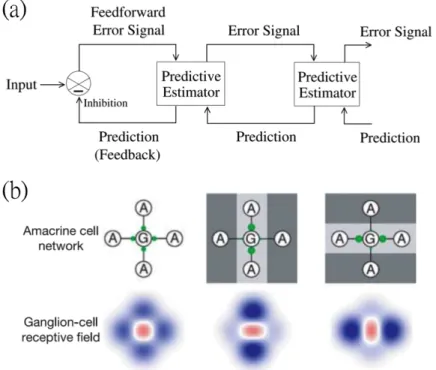
1.3 Anticipative responses. (a) Neural activities in the zebra fish larvae tectum maintain the periodicity after entrained by periodic moving bar stimuli (green vertical time stamps on the grey region). Fluores- cence from calcium imaging and the detected spikes are plotted for a population of cells. Purple lines indicate the same periodic pattern as the green lines but without visual inputs. The three arrows after entrainment indicate the OSR events. Figure reprinted from [88]. (b) Moving speed of a population of slime molds under periodic change in temperature (TM) or humidity (HU). The three arrows indicate OSR events after the periodic entrainment shown in grey regions. Note that similar patterns could be “recalled” after providing another input after a delay, indicated by white arrows. Figure reprinted from [72]. . . 8 1.4 Predictive coding in the retina. (a) A shamanic diagram for pre-

dictive coding. The input is compared or canceled with a feedback inhibitory signal, forming an error signal. The error signal is then feed to the predictive estimator, which generates the predictive negative feedback. Only the error signals are sent to the next stage in this hierarchical network structure. Figure reprinted from [68]. (b) An anti-Hebbian network that implements the dynamic predictive coding in the retina. The receptive field integrates the contribution from amacrine cell network. The inhibitory strengths, indicated by green circles, from the amacrine networks adapt to the input spatial pattern. Figure reprinted from [38]. The adapted network forms a

(14)

1.5 Predictive information in the sensory population. (a) Mutual information I(Wt; Xt+ t) is measured from the stochastic moving bar position xt at time t and retinal firing pattern Wt+ t at time t + t formed by spikes in N neurons. Note that the values at positive t time shifts are the predictive information measured from the current spiking pattern in time window ⌧ and the future stimuli, and the values are non-zero in this case. Figures reprinted from [65]. (b) Multiple stochastic moving bar trajectories that converge onto two certain paths are drawn in red and blue. Note how the corresponding firing patterns diverge when the trajectories are exactly separated at t = 0. These responses are further compared to the statistical limit to predict and separate these two future trajectories, as discussed in

the discussion section. . . 13

1.6 Division and relation chart of the thesis. . . 15

2.1 Block diagram for experimental methods. . . 17

2.2 Experimental setups . . . 19

2.3 Setup for spatial stimuli: The image on LCD is focused on the the MEA through lens and imaged by a camera. The instruments are fixed on the optic table. . . 20

2.4 MEA recording and Spike detection . . . 21

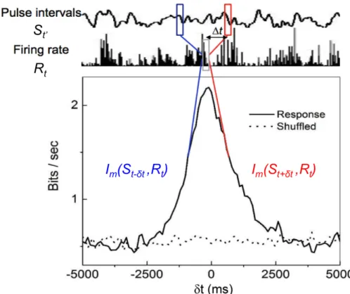
2.5 Measuring Im(S, R, t). Pulse intervals St⁰ and response firing rate Rt are used to calculate mutual information, where t⁰ is t shifted from t. The curve shows measurement under diﬀerent t shifts between two series. Blue parts on the left shows Im between response and stimuli in the past and red part on the right shows Im between response and stimuli in the future. Dot line is calculated from shuﬄed data, showing a biased baseline due to finite sampling that would be described in the following section. . . 25

(15)

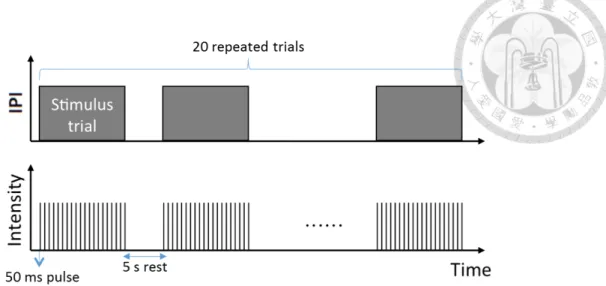
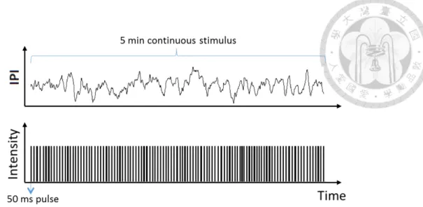
2.6 Protocol for periodic stimuli. Inter-pulse-intervals (IPI) are fixed in each trial. . . 27 2.7 Protocol for stimuli with stochastic intervals. Inter-pulse-intervals

(IPI) is generated by a correlated stochastic process. . . 28 2.8 3D phase portrait of AFHN model. The cyan volume is where the

system is in an oscillatory state, red trajectory is driven by external stimuli, and the deep blue trajectory is when the stimuli is terminated. Note that the deep blue trajectory continues oscillating before dropping to the fixed point. Figure reprinted from [98]. . . 32 2.9 Constructing LN model and STA . . . 34 2.10 PID model: An error signal e is feedback by comparing the input

signal r and output y. Operations sum up the proportion of error term, its integral throught time, and the derivative to adjust the output (https://www.wikiwand.com/en/PID_controller). . . 36

3.1 Firing patterns under periodic stimuli and OSR . . . 38 3.2 Four response types from diﬀerent units under the same periodic stim-

uli. (a) facilitation, (b) sustain, (c) period double, (d) silent types are recorded. The stimuli are 20 periodic pulses with period=170 ms shown at the bottom. . . 39 3.3 Dynamics of firing pattern under diﬀerent stimuli with diﬀerent pe-

riod. (a) period=140, (b) period=180, (c) period=220 ms. The upper figures are heat map for 19 sorted units and the bottom ones are average PSTH. . . 39 3.4 The latency of OSR depends on the period of stimuli. Response

(16)

3.5 3-pulse dose not produce well-timed OSR. (a) Three pulses in the upper plot and a sustain light in the lower plot are used as control experiments and the average PSTH for 20 channels are plotted. It is shown that the post-stimulus firing are diﬀused and less synchronized.

(b) The response delay has little dependency on period of the 3-pulse stimuli and the standard deviation across 20 channels are plotted. . . 41 3.6 OSR under long pulse intervals. (a) Raster plot with 17 trials showing

average firing rate from 20 sorted units under periodic stimuli with period=220 ms. (b) Average PSTH plotted for the same data set in (a). . . 42 3.7 OSR under dark pulses. (a) PSTH showing the average firing rate

from 21 units under periodic dark pulses with period=250 ms shown at the bottom. (b) The response latency of OSR under dark pulses with different periods. (c) Effect of duty cycle of the same periodic input with period=200 ms (12.5% duty cycle means that the pulse width is 25 ms and inter-pulse-interval is 175 ms) calculated with 11 units. . . 43 3.8 Effects of jitter temporal patterns. (a) to (c) are the average PSTH of

11 units under periodic stimuli with 20, 30, 40% of jittered percentage in pulse intervals, with mean of period=200 ms. (d) Response laten- cies of OSR under stimuli with diﬀerent jittered percentages. Mean of periods are fixed as 200 ms in each experiment. . . 44 3.9 Eﬀects of the last interval. (a) The period of stimuli in the first 18

intervals are 170 ms and the last interval (19^th) is 200 ms. (b) The period of stimuli in the first 18 intervals are 200 ms and the last interval (19^th) is 170 ms. The mean of response latency of OSR is 280 ms in (a) and 330 ms in (b). 59 units are used in the PSTH. . . 45

(17)

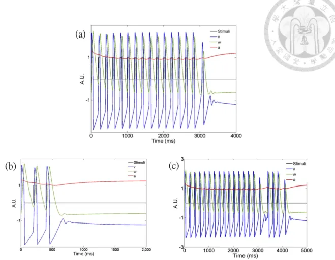
3.10 Eﬀects of the last pulse intensity. (a) PSTH under bright pulses, (b) dim pulses, (c) normal pulses with the last bright pulse, (d) normal pulses with the last dim pulse, (e-f) mismatched dim and bright pulses with diﬀerent orders. The averages firing rates are calculated from 20 units and the period=220 ms for all experiments. The mean response latency of OSR in (a)=310, (b)=290, (c)=370, (d)=295, (e)=345, (f)=305 ms. Note that those ending with brighter pulses in (c) and (e) have longer latency than those ending with dimmer pulses in (d) and (f). . . 46 3.11 AFHN model and the probed OSR. (a) AFHN model driven by pe-

riodic square waves. Note that an OSR-like activity in parameter v occurs after the last pulse. (b) Three pulses is not suﬃcient to produce an OSR under certain parameters. (c) When the same probe shown in (b) is placed after a longer entrainment with a delay time, the probe induces another OSR activity. . . 47 3.12 Probing OSR: (a) The designed stimuli to probe OSR after a de-

lay to the periodic entrainment. (b) The 3-pulse probe that dose not produce well-timed OSR, as mentioned in Fig. 3.5. (c) The same probe placed after a longer periodic entrainment induces another OSR. PSTH are plotted with the same 11 recorded units and the period=180 ms for both the probe and the entrainment. . . 49 3.13 Dependency of the probed OSR. (a) Response latency of the probed

OSR under diﬀerent period of probe (3-pulse stimuli that provides two intervals) with the same entrainment period=180 ms. (b) Re-

(18)

3.14 Control experiments for probed OSR. (a) Little probed activity after a short sustain light stimuli. (b) Larger synchronized firing after a long sustain light stimuli. The PSTH show average firing activities from 59 units. . . 51 3.15 Eﬀects of calcium concentration on OSR. (a) The response latency of

OSR probed by diﬀerent periodic stimuli after treated by EGTA. (b) PSTH under stimulation with period=300 ms after treated by EGTA, as shown in (a). 21 recorded units are considered in these two plots.

(c) The response latency of OSR under the same periodic stimuli with period=200 ms with diﬀerent concentrations of calcium in buﬀer. 30 units used for calculation. (d) PSTH under stimuli with period=200 ms after treated with EGTA-AM. Activity averaged from 10 recorded units. . . 52 3.16 PSTH for complex temporal patterns. (a) Periodic pulses with pe-

riod=180 ms. (b) “ABC” repetitive temporal pattern, where A=220 ms, B=180, C=140 ms. (c) Periodic stimuli with “A+B+C” period=540 ms. (d) Randomized “ABC” pattern with the same number of pulses and intervals shown in (b). Averaged activities are calculated from 59 recorded units. . . 54 3.17 Heterogeneous response to complex temporal patterns. (a) Heat map

for firing rates averaged over 20 trials from 60 channels. Horizontal axis starts from the timing of the last pulse. The upper plot is for ABC stimuli (A=220, B=180, C=140 ms) and lower plot is for periodic stimuli with period=180 ms (could be seen as “BBB”). Inset in each plot is the cross-correlogram for 60 channels calculated from the post-stimuli spike trains, with reddish color codes showing higher correlation coeﬃcients. (b) Average PSTH for the same sample shown in (a) that focuses on timing after the last pulse. Post-stimuli firing patterns for four stimulations plotted in Fig. 3.16 are shown. . . 55

(19)

3.18 Periodic stimuli with spatial patterns. (a) Whole field periodic stimuli. (b) Periodic stimuli that flashes a checkerboard pattern. (c) Periodic stimuli with each consecutive pattern showing an anti-phase checkerboard pattern. (d) Periodic stimuli that flashes random patterns with 50% white pixels randomly distributed. All the stimuli have period=100 ms and the average firing rate PSTH are calculated from 59 recorded units. . . 57 3.19 Stochastic pulse intervals and the induced retinal firing patterns. (a)

Time series of pulse intervals generated by the iteration formula; <

⌧ >= 200msand ⌧cor = 2s. (b) Raster plot showing firing timestamps from 60 channels under the input shown in (a). (c) Average firing rate of the population recorded in (b). To calculate mutual information, the stimuli shown in (a) with varying pulse intervals are defined as equally distributed 25 states shown in red. . . 59 3.20 An example of measured Im( t) with stimulation shown in Fig. 3.19.

Im( t) computed from shuffled data I_m^s( t) is also shown to serve as a base line. Three different measurements obtained from three sorted signals in the same experiment are shown in the inset to demonstrate the variability of the data. The bias due to limited sampling has been corrected for the all measured and shuffled data shown here. . . 60 3.21 Comparison of the three Im( t) as described in the text and the def-

inition of predictive power (Pp). Note that both Im(S, S, t) and Im(R, R, t)are symmetric about their respective peaks but Im(S, R, t) is not symmetric (inset). The oscillation observed in Im(R, R, t) is

(20)

3.23 Eﬀects of ⌧cor. (a) ⌧cor = 0.2s, (b) ⌧cor = 2s, (c) ⌧cor = 4s. The upper row are plots for average PSTH and the corresponding states of stimuli as shown in Fig. 3.19. The lower row shows Im( t) calculated for 5 sorted units selected from the upper plots. . . 64 3.24 Predictive power (Pp) depends on the statistical properties of the

simulation light pulses. (a) Measured Pp as a function of < ⌧ >

with ⌧cor = 10 < ⌧ > for each < ⌧ >. t-test indicates significant diﬀerence between values at < ⌧ >= 200ms and < ⌧ >= 300ms.

(b) Measured Pp as a function of 1/⌧cor with < ⌧ > fixed at 200 ms.

Note that Pp is computed from the mutual information measurements after bias correction. By applying t-test, Pp under < ⌧ >= 200 ms is significantly higher than those under < ⌧ >= 275 ms and < ⌧ >= 300 ms. For the eﬀects of ⌧cor, Pp under 1/⌧cor = 0.05 is significantly higher than under 1/⌧cor = 5. The results are obtained from the same retina, and the error bars indicate the deviation between 17 sorted signals. Specifically, 2 out of 19 channels are excluded after the validity check mentioned in the main text. The deviating performance might signify diﬀerent response types under stimulation with large

⌧cor. Note that the conclusions of our statistical tests are not aﬀected by this validity check. . . 65 3.25 Latency to peak tp of Im( t) as a function of ⌧cor obtained from 19

sorted units in the same retina. The left inset shows the definition of tp and the measured Im( t) with ⌧cor = 0.2 (blue), 2 (red), and 4 s (black). Right inset shows the relation between tp and Pp (bias corrected for limited sampling) calculated from the same data. By applying t-test, we find that tp is significantly diﬀerent for 1/⌧cor = 0.24 and 1/⌧cor = 5 . . . 66

(21)

3.26 Discriminating OU process and the HMM by a retina. Measured Im( t) with stimulations generated from an OU process (red) and an HMM (black), each with two diﬀerent correlation times. Comparison of tp under the two diﬀerent types of stimulations with varying ⌧cor

is shown in the inset. All measured mutual informations are bias corrected for limited sampling. . . 67 3.27 Performance under AR model stimuli. Measured Im( t) with stim-

ulations generated from AR model with longer (⌧cor = 8s, red) and shorter correlation time (⌧cor = 2s, black). Note that there are two peaks near t = 0. . . 68 3.28 Linking predictive information and OSR. (a) Average PSTH for OSR

type firing pattern under stimuli with period=200ms. 16 recorded units are calculated. (b) Average PSTH for sustain type firing patterns under the same stimuli as (a). 10 recorded units are calculated. (c) Im( t) calculated from 5 units selected from the OSR type shown in (a). For the stochastic stimuli used, < ⌧ >= 200ms and

⌧cor = 2s. (d) Im( t)calculated from 5 units selected from the sustain type shown in (b). The same stochastic in (c) is applied. (e) Peak of Im curve in two firing types analyzed from 16 units in (a). t-test indicates significant diﬀerence between two distributions (p<0.0001).

(f) Peak position tp in two firing types analyzed from 10 units shown in (b). . . 70 3.29 LN model for bullfrog retina. (a) The biphasic STA obtained by

reverse correlation. (b) Nonlinearity that controls the firing rate. (c)

(22)

3.30 LN model under stochastic pulse intervals. (a) Im( t)calculated from predicted response and the input stimuli. Mean of intervals is fixed as 200 ms and ⌧cor is 2s (black) and 8s (red). (b) Pp measured under diﬀerent mean of intervals with ⌧cor = 2s. (c) Pp measured under diﬀerent ⌧cor with mean of intervals fixed as 200 ms. . . 72 3.31 AFHN model under stochastic stimuli. (a) Im( t) calculated for

AFHN model that receives stochastic pulse intervals with < ⌧ >=

200ms. Two ⌧cor are used, 2s shown in red and 8s shown in black.

Note that tp dose not shift to a positive value even when the correlation time long. (b) Pp for variable v and a under stimuli with diﬀerent correlation time with mean fixed at 200 ms. (c) Pp for variable v and a under stimuli with diﬀerent mean of intervals with correlation time fixed at 200 ms. . . 73 3.32 Comparison of Im( t) with modeled response. The experimental re-

sult (with parameters the same as those in Fig. 3.19) is shown in black. The red curve is obtained from the LN model. The blue curve is obtained from linear extrapolating the input time series. These Im( t) curves are normalized by their peak values for the ease of comparison. . . 74 3.33 Gedanken retina for time series prediction. (a) Response generated

from the gedanken retina to predict the input time series. (b) Asym- metry and shift of peak of Im(S, R, t) where R is numerically produced by the gedanken retina aiming to estimate a future stimulus.

In producing the response R⌧ n, the gadenkan retina targets the future that is N steps ahead of the current stimulus. The input signal is produced from the same HMM process used in experiments. Note that the peak of Im(S, R, t) moves to the positive time shifts and decreases as the retina attempts to predict further into the future. . 76

(23)

3.34 Performance of PID controller. The Im(S, R, t)measured with HMM stimuli as S and PID operated signal as R can produce a positive time shift. . . 76

4.1 An oscillatory circuit that models OSR. The ON bipolar pathway is modeled by an adaptive oscillator that tunes its frequency according to the periodic input. The OFF bipolar pathway is a desensi- tized and rectified input signal. After passing through a threshold that is eﬀectively the firing threshold of the retinal ganglion cell, this model produces similar OSR patterns observed in the experiments.

The vertical green line indicates the omitted stimulus timing. Figure reprinted from [33]. . . 80 4.2 Retinal firing pattern encodes information for escape behavior in bull-

frogs. (a) A stereotypic escape behavior is observed in bullfrogs when an expanding visual stimulus is presented. The escape rate in behavior is significantly deprived when the antagonist of GABA receptors (Bicuculline, Bic) is injected in both eyes. (b) MEA recording for firing patterns from the dimming detectors in bullfrog retina under the same expansion stimulus. While the total firing rate is not af- fected in the PSTH, regularity of inter-spike-intervals are disrupted when treated with Bicuculline. These results show the importance of retinal synchronized oscillatory firing pattern in escape behavior and reveal the essential role of inhibitory neurons in the retina. Figure reprinted from [40]. . . 82

(24)

4.3 Optimality of predictive information in the retina. (a) Information about the future stimuli (distinguished at t = 0) from t time lag behind, calculated from firing pattern of 5 retinal ganglion cells. The solid line shows the statistical limit to predict this stimuli estimated by the IB method. (b) Shows the optimality of groups with diﬀerent number of cells N, plotting information captured for the past Ipast

against the predictive information If uture at a fixed t timing. The solid line is calculated from the IB method, showing a bound on predictive information (If uture^⇤ ) given an encoded past. Note that the If uture/I_{f uture}^⇤ is close to 1 in the results, indicating the optimal performance for prediction. Figure reprinted from [65]. . . 88 4.4 Population firing rate as a coding strategy. (a) The OSR response

types are identified and stimulated by stochastic stimuli same as Fig.

3.28. The peak values of Im curves are plotted against the number of units considered in the population firing rate code from OSR type.

This neural code constructed by simply adding up the firing rates from the sampled units. Each error bar is plotted for 15 subgroups resampled from 10 recorded units. (b) The same calculation for 10 units of sustain response type. . . 91

A.1 Eﬀects of AP5. (a) OSR is recorded in the population average firing pattern from 59 units. The period of stimuli is 140ms. (b) The same units recorded under the same periodic stimuli after treated with AP5.106 A.2 Eﬀects of Bicuculline. (a) Average firing rate pattern from 59 recorded

units under the “ABC” repeating stimuli, where A=220ms, B=180ms, C=140ms. (b) The same units responding to the same input after treated with Bicuculline. Note that the firing rate is lower and it increases and saturates faster than the pattern shown in (a). . . 106

(25)

B.1 Other coding strategies. (a) Im curve calculated from three diﬀerent neural coding strategies. Rate coding is the method used in this study, binary method is ignores the firing rate and reduces it into binary reposes, and WTA method selects the unit that fires first in the subgroup. Here we use 5 units in the WTA method. The stimulus has the same statistics as described in Fig. 3.19. (b) The peak value in Im curves calculated from WTA method depends on the number of units sampled. Each error bars reflects the deviation in the 15 resampled subgroups from 11 recorded units. . . 108 B.2 Statistics for stochastic processes. (a) A schematic diagram for itera-

tion processes in OU and HMM, shown in equations 2.5, 2.6, and 2.7.

It is shown that each step in the OU process solely depends on the last consecutive iteration. In contrast, there is a hidden “velocity” term that connects the last two steps and determines the next iteration, shown in the purple region. (b) The autocorrelation of two stochastic processes with similar half-time, approximately 2s. (c) Im(R, R, t) calculated from two stochastic processes, with the same statistics as shown in (b). . . 109 B.3 Calibrations for information measurements. (a) The peak value of

I_m curve plotted against the bin size for spike trains. The stochastic stimuli has < ⌧ >= 200ms and ⌧cor = 2s. (b) The same unit recorded from the same stimuli in (a), with peak value of Im curve plotted against the number of states defined for the stochastic process. (c) Peak values of Im curves are plotted against subsampling fraction

(26)

C.1 The black box that provides light stimulation and perfusion. (a) The stimulation box covered on the MEA system. (b) Bottom view of the box. Note that the box is turned up-right and covered on the MEA during experiment. (c) Two iron needles are inserted into the box, forming a holder for the perfusion system. . . 118 C.2 Steps for the retina dissection. 1. The bullfrog eyeball is isolated.

2. Two forceps are used for dissection. 3. One can use scissors to cut the cornea oﬀ. 4. The iris, vitreous gel, and lens are pulled out.

The retinal tissue could be gently pealed oﬀ from the sclera as well.

5. The pigment epithelium is separated from the retina. 6. The un-bleached retinal tissue should be pinkish. We further remove the remaining vitreous gel from this tissue before recording with MEA. . 119

(27)

Chapter 1 Introduction

1.1 Computation and Coding in the Retina

How the nervous system computes and represents dynamical stimulus are fundamental questions in neuroscience. Benefit from development in neural technologies, it is possible to record activities from neural population in real-time and manipulate specific subsets of cells in the network[82, 17]. However, complex recurrent structures and diverse response types may hinder the understanding towards neural dynamics in the brain[41]. Early sensory systems, on the other hand, provide a relatively simple and accessible platform that enables the study of generic phenomena and biophysical mechanisms across nervous systems. For instance, neural responses in the visual, auditory, olfactory, and somatosensory systems could be recorded under controllable stimuli, allowing us to explore the neural code that represent the corresponding input signals[70]. Specifically, the retina has been an ideal model for these studies, since the cell composition and circuits are relatively well-studied[48, 51].

Recording methods for a population of retinal activity and computational description of the retinal circuits facilitate our understanding for computation and coding

(28)

cells (⇠ 2 types), bipolar cells (⇠ 12 types), amacrine cells (⇠ 30 types), and the ganglion cells (⇠ 20 types)[51]. Note that these five main types are preserved across vertebrates and the number of subtypes in parenthesis is an approximation for mam- malian retina. Light signals are transformed into change in membrane potential, namely phototransduction, starting in the photoreceptor cells through biochemical signal pathways. These signals are sent to horizontal cells and bipolar cells. The horizontal cells forms the inner nuclear layer and provide negative feedback to the surrounding photoreceptors. Bipolar cells transmit signals to the ganglion cells, but can invert the response phase, forming ON and OFF pathways. Bipolar inputs are innervated to the inner plexiform layer, where they connect to the amacrine cells and retinal ganglion cells. Amacrine cells receive signals from multiple parallel units mediated by bipolar cells across the horizontal axis, inhibiting lateral bipolar termi- nals and ganglion cells. In the last stage, retinal ganglion cells integrate inputs from bipolar cells and amacrine cells, then produce action potential that projects to the next stage in the visual system (Fig. 1.1). Note that this is a general description for signal processing in the retina that discards a number of physiological details, such as electrical coupling between cells and long-range modulatory signals[12, 97].

The cell types and connections are critically related to its functional properties. For instance, parallel processes of diverse bipolar cells are sampled by diﬀerent types of ganglion cells, forming feature selection in diﬀerent channels[28]. Lateral and feedback inhibition from the amacrince cells regulate ganglion activities in space, developing array structure and direction selectivity[46]. Many studies attempt to describe these circuits with functional units. “Receptive fields ” are defined by the area in space where the neuron receives input from[42]. Classical receptive fields of a retinal ganglion cell forms a “center-surround” structure. Light signals that fall in the center and surround regions may evoke opposite response in the ganglion cell, possibly forming a “Mexican hat” spatial kernel that enhances spatial contrast through lateral inhibition[2]. These operation on spatiotemporal signals could be approximated as a linear filter that weights the stimuli across space-time before

(29)

Figure 1.1: Structure of the retina. Five layers of cells are shown in the retinal tissue on the left. Light is projected from the bottom in the physiological condition.

Examples of the evoked activity in membrane potential of diﬀerent cells are shown on the right. Note that G1 and G2 ganglion cells firing in a diﬀerent phase due to the inverted signal in their upstream bipolar cells. Also, only amacrine cells and retinal ganglion cells produce action potentials. Figure reprinted from [26].

summation (summing across the dynamics range of multiple bipolar channels). To convert these analog signals to spiking activities generated in the retinal ganglion cells, the linear-nonlinear model adds a nonlinear function or threshold that approxi- mates the eﬀective spiking threshold to the filtered signal[23]. This simplified model can characterize certain retinal activities and parameters could be fitted through experimental data. However, the static parameters and reduced functional units fails to capture a number of retinal function.

A set of generic neural computations has been observed in the retina, including adaptation, detection, and prediction[36, 44]. These phenomena could not be

(30)

cise timing between spikes from ganglion cells are shown to be crucial in encoding spatial patterns[35]. For prediction, it is shown that the retina could anticipate the motion of a moving bar, periodic light flashes, and adjusts its receptive field structure dynamically according to the stimuli in a predictive manner[4, 78, 77, 38].

Furthermore, one of the main goals in computational neuroscience is to eventually understand these neural codes in a population level as well. Pair-wised interactions, synergy and redundancy, thesaurus for population code, thermodynamic signatures, and robust “modes” of population firing patterns have also been discovered in the retina[74, 75, 32, 89, 67].

In this study, we focus on prediction and coding for temporal patterns in the retina. Following up the studies on sophisticate temporal patterns observed in retinal activities, we sought to compare these phenomena with an adaptive model, quantify the performance of temporal prediction, and generalize the measurement under more complex temrpoal patterns. Linking to the aforementioned aspiration in neuroscience research, we expect that these observed phenomena and analytic methods could be realized in other nervous systems.

1.2 Omitted Stimulus Response

Neural responses change dynamically under repetitive temporal stimulations. Be- sides habituation that decreases in response amplitude over time, facilitation and complex patterns known in chaotic dynamics could also be observed from the nonlinear responses to periodic stimuli[77, 30]. It has been shown that the transient response to change in these input pattens reflects the ability in detection and prediction. Event-related potential evoked by termination of periodic entrainments or presentation of “oddball” signals has been recorded in diverse brain regions under diﬀerent sensory inputs. For instance, a mismatch negativity (MMN) signal has been recorded from the local field potential of cortex when a diﬀerent frequency suddenly appears in a series of same tones[59, 71]. The robust response signature similar to MMN is conserved across species, reflecting the crucial function for nervous systems

(31)

to detect temporal patterns. It could also be used as a marker for diagnosis in cognitive function. In fact, such phenomenon is closely related to predictive coding strategy that focuses on the coding for unpredicted “surprise” in the input[92, 71].

In other words, the reaction is significant when the input diﬀers from the expected pattern, forming a representation that predicts the ongoing stimuli.

Surprisingly, similar phenomena were observed in primary visual systems such as the tectum and retina in early studies, showing omitted stimulus potentials after periodic stimuli[20]. Further investigations provide evidence that pattern detection and prediction already exist in the retinal firing patterns, where the visual information is first operated in the nervous system[78, 77] (Fig. 1.2). This implies that a relatively simple neural circuit would be suﬃcient to encode and predict temporal patterns. Under the same periodic light stimuli, firing patterns of retinal ganglion cells exhibit various adaptive patterns. The omitted stimulus response (OSR) is recorded from the firing of retinal ganglion cells after a periodic light flash. OSR usually increases in firing rate comparing to the activity during periodic entrainment. Importantly, this significant firing pattern is not an arbitrary oﬀ response to the terminated stimuli, but is precise in time and reflects the entrained periodicity.

The latency of OSR to the last pulse increases linearly as the interval of periodic flashes lengthens in certain range. In fact, the update of OSR latency can be sen- sitive to change in pulse intervals as short as 5 ms. In other words, OSR seems to precisely predict when the upcoming pulse should have occurred in time.

OSR is a robust signature for temporal prediction in the retinal circuit across species[20, 78, 53]. The behaviors of OSR cannot be described by classical retinal models such as the linear-nonlinear model mentioned in the last section. Models to

(32)

Figure 1.2: OSR phenomenon. (a) The visual-evoked potential (VEP) and omitted- evoked potential (OSP) recorded from the optic tectum in fish under periodic light stimuli. Note that VEPs adapt to high frequency and strong oscillatory OSPs occur after the periodic stimuli. Figure reprinted from [20]. (b) Firing rate increases when the periodicity of the light flashes is disrupt, and this phenomenon is conserved across species. OSR is defined by the increase in firing rate after the periodic stimuli. The relative latency from the last pulse to the timing of OSR is linearly related to the stimulus period. Figure reprinted from [78].

from repeating the classic OSR measures in the bullfrog retina and further explore the ability in temporal coding and prediction.

1.3 Anticipatory Response with Adaptive Dynamics

Entraining neural activities with external stimuli is similar to the generic phase synchronization phenomenon in dynamic systems[86]. A similar period to the periodic input signal can be observed in entrained system under certain coupling to the stimuli. For instance, physiological responses that follow the daily period in cir- cadian rhythm would be a significant example in biological systems[19]. However, diﬀerent from physical systems, rather than moving back to its initial period when external drive removed, biological systems are not only able to retain memory of the un-driven system but also generate additional activity after the termination of signal. MMN described in the last section is an typical example. In other cases such as working memory and sensory memory, it has been shown that dynamics of external stimuli can temporally pertained in the system. Previous research performed

(33)

either in vivo or in vitro experiments on auditory and visual systems to demonstrate similar abilities[88, 34, 5].

One of the noteworthy examples is the entrained rhythmic activities in zebra fish larvae [88]. It is shown that the periodic light entrainment could be maintained in certain neural ensembles in the tectum even after the stimuli stops. Similar to the well-timed behavior in OSR, the intervals depends on the entrained periodicity.

Furthermore, the induces ocular motion in zebra fish larvae can also maintain the periodicity. This indicates how biological system can perceive time intervals across diﬀerent nervous systems and actively maintain the entrained temporal patterns.

On the other hand, another example could even be found in non-nervous systems such as slime molds[72]. The velocity of slime mold motions could be periodically tuned by temperature in the environment. It is shown that these slime molds can not only maintain the periodicity in motion velocity but also recall the previously entrained period after a certain delay time (Fig. 1.3). These phenomenon are generic in biological systems across diﬀerent scales and species. In fact, besides viewing the activity as preserved “short-term memory” of temporal information, another interpretation is that it anticipates the upcoming periodic input.

Many have attempted to model these anticipatory responses for temporal patterns. Reservoir computation methods such as populations of oscillators and scale free network with multiple recurrent loops could simulate behaviors observed in the experiments[56]. However, as for behaviors such as OSR recorded in the retina, these assumptions for large number of computational units might not be valid. An- other possible strategy might be adaptation. There are a number of candidates for adaptive dynamics to occur in the retinal circuits, such as synaptic strengths

(34)

Figure 1.3: Anticipative responses. (a) Neural activities in the zebra fish larvae tectum maintain the periodicity after entrained by periodic moving bar stimuli (green vertical time stamps on the grey region). Fluorescence from calcium imaging and the detected spikes are plotted for a population of cells. Purple lines indicate the same periodic pattern as the green lines but without visual inputs. The three arrows after entrainment indicate the OSR events. Figure reprinted from [88]. (b) Moving speed of a population of slime molds under periodic change in temperature (TM) or humidity (HU). The three arrows indicate OSR events after the periodic entrainment shown in grey regions. Note that similar patterns could be “recalled” after providing another input after a delay, indicated by white arrows. Figure reprinted from [72].

parameters of STSP could be generalized by facilitation and depletion factors in the synapse, which may majorly correspond to the calcium influx and release of neural transmitter due to neuronal firing activities. Coupling with recurrent firing event of the neurons, this synaptic model generates spontaneous activity that can be implemented as working memory. In fact, following an proposed model, the adaptive FitzHugh-Nagumo model, the synaptic model can be an analogy of an adaptive excitable system[98]. This conceptual model describes the “time perception” and

“anticipation” of OSR. Rather than utilizing any biological “clock ” to record timings or including a large population of cells, the facilitation of synapse can already adapt to the temporal patterns of input and maintain its dynamics after removal of stimuli. These descriptions will be included in the discussion and comparison for OSR observed in retina experiments.

(35)

1.4 Prediction and Predictive Coding

The ability to predict or anticipate future events is crucial for the survival of animals. Predicting dynamical inputs can compensate the latency during neural signal transfer and provide predictive information for learning and guidance for behavior[9, 4, 14]. In behavioral studies, it is shown that predators could predict the moving prey in order to capture it efficiently[14]. In the visual cortex, entrainment by spatiotemporal patterns have long-term effects on how the neurons react to different sequence of inputs, reflecting the ability to recognize and predict sequen- tial events[34]. In fact, a number of abilities to make prediction could be found in the early stage of sensory systems such as the retina[3]. For instance, the retina anticipates moving stimuli by firing near the leading edge of the moving bar. Such anticipative response in front of the moving object has been modeled by known retinal circuits and also implemented in continuous neural networks[57, 4]. In the population level, retinal populations provide prediction about the position of a moving object in the future. This target-tracking circuit enables the brain to extrapolate moving objects through linear decoding methods and guides the eye or head move- ments efficiently[47]. These discoveries emphasize the ability to make prediction in the retina and also reveal crucial functions that are physiologically (to compensate the main latency due to neural transmission) and ethologically (for prey tracking) relevant.

While making prediction eﬃciently has been thought as a main principle in neural coding, a specific strategy called predictive coding building upon this principle has been proposed[68, 84]. Such strategy operates by predicting the future states, fo-

(36)

shown in diﬀerent cortical areas[31]. This hierarchical connection allows prediction from higher levels to feedback and inhibit activities in the lower levels, only sending signals with predictive error to the consecutive stage in the network. This cen- tral scheme of predictive coding forms an eﬃcient representation for unpredictable signals in each stages.

Dynamic predictive coding starts from the retina. The receptive field adaptively changes its weightings in the spatiotemporal filter according to statistics of the stimuli (Fig. 1.4). For instance, after adapted to images with horizontal straight lines, the receptive field habituates in the horizontal axis and sensitizes in the vertical axis. In other words, if the retina is exposed to the unexpected vertical line stimuli, the response will be more significant that those continued under horizontal lines.

This behavior could be explained by an anti-Hebbian circuit that inhibits the input signal when it is adapted, similar to the concepts for predictive coding in the cortical circuits[38]. While the properties for receptive field have been studied, how similar dynamic predictive coding under temporal patterns happen in the retina is less known, and methods to quantify this phenomenon is required.

1.5 Predictive Information

Spiking patterns are universal codes in the nervous systems. Input signals are rep- resented and transmitted by this discrete digital-like neural activity. Fundamental issues in computational neuroscience are to understand how these spike trains encode information, measure the reliability, and develop methods to quantify it by applying information theory[70]. Information contained in the spike train turns out to be important to understand the functions from single neuron, networks, to behavioral scales[70, 6, 7]. Particularly, many have attempt to understand the neural codes in the retina for visual inputs. Encoding through combinatorial codes in the cell population, information rate transmitted by firing patterns, and the maximal informative encoding in diﬀerent cell types have been studied in the retina[6, 76, 45]. More re- cently, a measure called predictive information has been applied to characterize the

(37)

Figure 1.4: Predictive coding in the retina. (a) A shamanic diagram for predictive coding. The input is compared or canceled with a feedback inhibitory signal, forming an error signal. The error signal is then feed to the predictive estimator, which generates the predictive negative feedback. Only the error signals are sent to the next stage in this hierarchical network structure. Figure reprinted from [68]. (b) An anti-Hebbian network that implements the dynamic predictive coding in the retina.

The receptive field integrates the contribution from amacrine cell network. The inhibitory strengths, indicated by green circles, from the amacrine networks adapt to the input spatial pattern. Figure reprinted from [38]. The adapted network forms a receptive field that is desensitizes to the original input but sensitizes to the orthogonal one, similar to the predictive coding scheme in (a).

(38)

predictive behaviors[65].

Information is a quantitative measure for uncertainty. Similar to entropy in thermodynamical systems, Shannon entropy of a variable is calculated from the probability distribution of its configurations[24]. For instance, a fair coin would have a maximal entropy since the possibility for heads and tails are equal likely, while a biased one would have be less uncertain due to a biased weighting in the probability. In another perspective, one needs more information to make a proper guess for a fair coin, while information about the biased distribution would significantly narrow down the uncertainty for the biased coin. Built upon this idea, one can also measure the mutual information between two random variable. Mutual information quantifies how much information could be conveyed about one variable given the other variable. Similar to correlation measurements for linear systems, mutual information is therefore commutable, but can well characterize nonlinear relations. It is therefore an ideal method to quantify neural encoding in terms of bits, by measuring the mutual information between the given stimuli and the evoked neural activities.

Predictive information is the mutual information between the past and the future events[10]. It measures how much one can predict the feature states by knowing a certain range in the past. Predictive information has been applied to physical systems and it relates to the measure of complexity and models for Baysien learning[9].

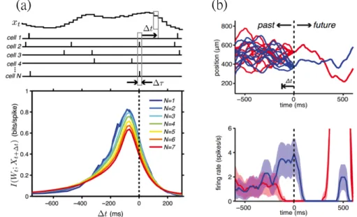
This measure was applied to activities recorded from H1 neurons in the fruit fly and retina of the salamander[11, 65] (Fig. 1.5). Combined with the information bottleneck method that quantifies the physical bound for a system to make prediction under the given correlated stochastic stimuli, these works demonstrate the optimality for the sensory systems to make prediction. This quantity, however, dose not reveal the underlying mechanisms for the sensory system to do so. It would also be interesting to see how the performance changes as the input statistics vary.

(39)

Figure 1.5: Predictive information in the sensory population. (a) Mutual information I(Wt; Xt+ t) is measured from the stochastic moving bar position xt at time t and retinal firing pattern Wt+ tat time t + t formed by spikes in N neurons. Note that the values at positive t time shifts are the predictive information measured from the current spiking pattern in time window ⌧ and the future stimuli, and the values are non-zero in this case. Figures reprinted from [65]. (b) Multiple stochastic moving bar trajectories that converge onto two certain paths are drawn in red and blue. Note how the corresponding firing patterns diverge when the trajectories are exactly separated at t = 0. These responses are further compared to the statistical limit to predict and separate these two future trajectories, as discussed in the discussion section.

(40)

1.6 Organization of the Thesis

This work focuses on the predictive response to temporal patterns in the retina. The experiments can mainly be divided into two parts, which investigate the transient and continuous responses. For transient response, we repeat experiments to record OSR and explore the underlying mechanisms by designing stimulation with diﬀerent temporal patterns. The results are compared to a previously proposed models to verify some of the predicted behavior in OSR. While OSR is probed by periodic stimuli, we provide complex patterns with multiple periods and also generate intervals through stochastic processes with controllable statistical properties. This leads to the analysis in stationary responses. Information theory is introduced to analyze the response under stationary stochastic pulse stimuli and characterize predictive behavior in the retina. Predictive information under stochastic temporal patterns were quantified and the dependency to statistics of the stimuli were demonstrated.

We attend to bridge the observation in transient response and measurement under stationary process. Also, schematic models to predict stochastic temporal patterns were proposed. Finally, possible biological mechanisms for predictive coding in the retina are discussed and compared with other models and observations in the nervous system. A schematic diagram in Figure 1.6 shows the aforementioned logic flow that links each experiment. The blue charts correspond to diﬀerent sections in the results. Each consecutive chart is connected by a related new question and should be answered with another method. Red charts on the right show the designed stimuli or method in each section, and the orange charts are topics investigated in the section.

(41)

Figure 1.6: Division and relation chart of the thesis.

(42)

Chapter 2 Materials and Methods

Systems and computational approaches were applied in this work. We performed electrophysiological recordings, designed stimulation, analyzed the recorded data, and implemented some of the experimental results through modeling. The experiments were performed by projecting light onto the bullfrog retina and recording activity with multi-electrode array (MEA). Extracellular activities of the retina were measured by the electrodes and action potential from the retinal ganglion cells were extracted. We compared these spiking patterns by calculating the spikes in a certain time window, namely the firing rate, under diﬀerent light stimulation. Timings of the spikes were identified and mutual information between the firing patterns and stimuli were quantified. The flow chart for these experiments are shown in Figure 2.1. For numerical modeling, both the classical methods to predict retinal responses from the experiment and an “gedanken” retina were simulated.

2.1 Sample Preparations

Retina samples were obtained from adult bullfrog. These frogs were kept in the lab with water circulation system. Before each experiment, the bullfrog would be dark-adapted for over 1 hour then sacrificed though double-pith operation. The eye ball was dissected and the retina was obtained under dim red light in oxygenated buﬀer. The sample was immersed in Ringer’s solution (NaCl 100.0, KCl 2.5, MgCl2

1.6, CaCl2 1.0, NaHCO3 18.0, Glucose 10.0 mM)[40] throughout the experiment.

The eye dissection procedure started with removing the cornea hemisphere with a

(43)

Figure 2.1: Block diagram for experimental methods.

sharp blade. After pulling out the lens, the vitreous humor and surrounding iris were gently detached from the sclera. A small patch of retina (approximately 2 mm x 2 mm) was cut and isolated. After removing the remaining vitreous gel and pigment epithelium, the tissue was transferred and placed on the MEA with the ganglion cell layer facing the electrodes. A piece of permeable membrane and anchor were then pressed on top to fix the retina sample. The retina was then kept in the MEA well and perfused with oxygenated Ringer solution with 1 ml/min flow rate at room temperature. The retina was recovered for another 30 minutes after these operation before providing stimulation. On average, the sample maintains its activities for 6-8 hours with such protocol[82].

2.2 Experimental Setup

(44)

fied (MEA1060-Inv-BC, Gain: 1100, Bandwidth: 1 Hz-3 kHz) then recorded by MC_Rack software with 20 kHz sampling rate in the computer[49].

For stimulation, except the inputs with spatial pattern, all experiments were conducted by providing light from a light emitting diode (LED) with 560 nm wave- length. LED illuminates the whole retina diﬀusively after hitting a beam splitter.

Across the 50%reflect-50%transmission beam splitter, half of the illumination would be recorded by a photodiode (HAMAMATSU S1223-01) to monitor the stimulation.

The final intensity of the light flash on the retina sample would be approximately 5 cd/m². In order to read in current from the photodiode and control the voltage across the LED, a data acquisition (DAQ, NI USB-6221 BNC) card is connected to the computer and programmed by MATLAB. The DAQ is connected to the LED, receives signal from the photodiode, and sends timestamps back to the computer during experiments. The photodiode is connected in parallel with a 10M⌦ resister to amplify and convert the current signal to voltage. Before every experiment, the voltage-intensity function was measured to calibrate the correct LED intensity for stimulation. The LED, beam splitter on a filter holder, and photodiode is mounted into a plastic black box. This box is then placed on the MEA recording system during experiments to prevent other indirect light (Fig. 2.2).

In one experiment with spatial patterns, the light source is a liquid crystal dis- play (LCD, 60 Hz) monitor focused onto the retina. The setup was fixed on the same optical table. After reflected by a mirror, the LCD image was focused by a 4X objective from the bottom of the MEA chip, which is transparent. The checkerboard pattern is achromatic and with the similar intensity as LED, calibrated by a pho- tometer (Fig. 2.3). Width of each pixel in the checkerboard is around 60 mm after focusing onto the retina, checked by taking a picture through a CCD camera from top. The visual input was programmed by Psychtoolbox-3 written in MATLAB[55].

(45)

(a) Stimulating and recording the retina. Left: The retina is stimulated by LED and recorded by MEA. Signals are received by and sent from the same computer. Right: The retina is fixed on the MEA with red plastic web.

(b) LED control: The LED is connected to the DAQ, which receives signal from the photodiode that measures the LED intensity. The LED, diode, together with the beam splitter in between, are fixed in a box that covers the MEA system.

Figure 2.2: Experimental setups

(46)

Figure 2.3: Setup for spatial stimuli: The image on LCD is focused on the the MEA through lens and imaged by a camera. The instruments are fixed on the optic table.

2.3 Signal Analysis

2.3.1 Data processing and validity check

Raw data recorded from MC_Rack software (.mcd file) was imported to MATLAB and analyzed by custom written programs. For preliminary data analysis, channel data were passed through a second-order high-pass Butterworth filter with a cutoﬀ frequency at 200Hz. This smooths out the low frequency fluctuation due to perfusion and from other layers in the retina. The spikes were then detected by using 5X standard deviation of the signal as a threshold. The crossing points are identified as spurious spikes. Each channel data are smoothed and detected separately.

To confirm the waveforms of these spikes, threshold crossing time were identified and a 0.5 ms pre-threshold period was extracted. We used a 1.6 ms window to perform spike sorting with these spurious spikes in the commercial Oﬄine Sorter software[82, 99]. By applying T-Dist E-M Sorting (T-Distribution Expectation Max-

(47)

(a) Filtered signals. Left: the raw filtered data from MEA recording shown in the MC_Rack software in real-time. Right: One filtered channel shown in the Oﬄine Sorter software. Two colors of spikes correspond to the sorted waveforms.

(b) Spike sorting. Left: Two clusters separated in the PCA projected feature space. Right: The corresponding waveforms sorted. The green wavelet is an action potential.

Figure 2.4: MEA recording and Spike detection

imization algorithm), diﬀerent waveforms were clustered automatically in the feature space (Fig. 2.4). This algorithm is agglomerative, proceeding through diﬀerent number of clusters and minimizes a penalized likelihood function. After sorting, the clusters were presented in the principle component space and multivariate ANOVA were applied to verify the statistic significance. On average, 10-20 clear waveforms can be sorted from a retinal sample for further analysis. Channel data with ambigu-

(48)

senting spiking events within a binning time and 0 for silence. The binning time used in this work is 5 ms for plotting the PSTH and measuring the timing of OSR.

Normally only one spike would be observed in this time bin, while we also scan over other bin sizes to compare the information contents. In the retina recordings, we can observe sparse spontaneous spiking patterns after the 30-minute dark adaptation.

Also, a series of pretest stimulation would be presented on each sample to confirm retinal functions, such as 1 second of sustain light stimuli and the flickering light for spike-triggered-average mentioned in the following sections.

In the experiments reported below, error bars in all the figures reflect the standard deviation between the recorded channels or sorted units. Therefore, the deviation must not be taken as the uncertainties of response from a single unit, which can be quite precise in time for OSR (within 5 ms). Since there are different cell types in the retina, there are strong variations in firing responses. A validity check was applied in the results under stochastic stimuli. As the mutual information between the response recorded by the MEA and the stimulation will be used in this work to quantify the predictive power of the retina, a channel was included for analysis only when its corresponding measurement was significantly (two times) higher than that obtained from its shuffled (time-randomized) version after the bias correction described below. In other words, we excluded channels which record firing patterns that share little information with the stimulation. Less than 25% of the selected units were removed after this validity check. We note that while the deviating per- formances of the removed channels might signify some different response types, the removal does not affect the conclusion of our statistical tests.

Besides the comparison between channels, the same experiment was tested with diﬀerent bullfrog retina as well, to confirm the reliability across individuals. Al- though results from one sample are shown in the following contents, for experiments on OSR, probe stimuli, complex temporal patterns, and the stochastic stimuli, each experiment was performed with more then 3 samples and the conclusions were the same. Those with diﬀerent responses in the pretest trials (for instance, high firing

(49)

rate in spontaneous activity or spontaneous oscillation that might reflect the injured retinal tissue) were discarded. On the other hand, experiments with dark pulses, pharmacological tests, and spatial patterns are preliminary results, repeated for less then 3 times and could be included in the future works.

2.3.2 Information theory

Information theory is applied to quantify the encoding performance of the retina or models. Similar to entropy in thermodynamics that quantifies the configuration in a system, Shannon entropy (H) conveys the information content in terms of bits, which quantifies the uncertainty of variables in binary states[24, 83, 87]:

H(X) = X

p(x)log2p(x) (2.1)

where p(x) denotes the marginal probability density drawn from the distribution of X. Given two random variables X and Y , we can also ask how much information they share with each other, namely the mutual information Im(X, Y )[16, 6]. This is calculated by the sum of their entropy minus the joint entropy. Derived from the definition of entropy in Eqn. (2.1), it can be written as:

Im(X, Y ) = H(X) + H(Y ) H(X, Y ) = X

X

Y

p(x, y)log2

p(x, y)

p(x)p(y) (2.2)

where p(y) is the marginal probability density of Y and p(x, y) is the joint probability density function of Xand Y. This operation in Eqn. (2.2) is commutable:

I_m(X, Y ) = I_m(Y, X), reflecting the mutually shared information content in bits.