應用卷積神經網絡於支氣管超音波影像診斷

(1)

國立臺灣大學電機資訊學院生醫電子與資訊學研究所碩士論文

Graduate Institute of Biomedical Electronics and Bioinformatics College of Electrical Engineering and Computer Science

National Taiwan University Master Thesis

應用卷積神經網絡於支氣管超音波影像診斷 Endobronchial Ultrasound Images Diagnosis Using

Convolutional Neural Network

藍偉任 Wei-Ren Lan

指導教授：張瑞峰博士 Advisor: Ruey-Feng Chang, Ph.D.

中華民國 106 年 8 月

August, 2017

(2)

口試委員會審定書

(3)

致謝

碩士生涯在我的任性下從兩年變成四年，原本還想離開工程轉向人文領域，

但最後還是選擇完成，才真的像是個研究生。首先，很感謝張瑞峰老師給予電子所逃兵的我機會，讓我能深入醫學影像領域。有別電路設計與人的距離遙遠，醫學影像處理與人的貼近有更多意義感。除了在意義感上做研究是個幸運，同時也有老師總是不嫌棄的指導研究方向，使得在研究上才能一步步跨過瓶頸並完成。

真的很謝謝老師。

還有個幸運是有很棒的實驗室，學長姐與同學們不吝於給予研究上的建議。

在一開始拿到影像資料時，感謝猴子、鴻豪學長們分享怎麼起步。由於是第一次撰寫論文，使用的描述跟語法很多不到位，小賢學長花了許多時間協助修正。假如沒有學長的耐心指導，我想自己是無法完成像樣的論文的。小賢很清晰分享論文每段落該有的重點，還有一些細節上的注意事項，這讓害怕無法畢業的自己覺得有希望。小賢學長，真的很謝謝你。很感謝柯南 Candy 小江謝恆立徐宏毅彭馨儀的接納讓我有個歸屬感，你們的有趣、善良使得我才能在最後失去好朋友的幾個月能支撐下去完成研究。最後很感謝我的父母這 20 幾年來打拼只為栽培孩子們，因為有你們當靠山我才有辦法到台大就學且能沒有壓力的做研究。還有感謝蕙慈在我轉所後這兩年很深入的陪伴，因為有你使我每次遇到瓶頸時能更有勇氣渡過。阿翔、焦品貴、丞嘉、邱媽、楊勳，也謝謝你們在我困頓時願意花時間跟我聊天，讓我能跟心中的憂鬱對抗而期待更好的自己。最後還有德濬、麋鹿、

小錡、大維、阿肥、林奕廷、puipui、庭碩、柏任、John、妮妮、Amy、嗯唉的大家們，與你們一起做過的事與對話，讓我這四年的碩班生涯真的很精彩與充實。

(4)

摘要

肺癌在美國是死亡人數最高的癌症，及早的治療，可有效提升肺癌的存活率。

支氣管超音波影像由於他的即時性、低輻射、較好的偵測能力，並且可與穿刺搭配常用來做肺部疾病檢查以及肺部病灶的良惡性診斷，近年來成為一個肺癌重要的診斷工具之一。不過目前病灶的支氣管超音波圖像判斷以醫生主觀統整特徵做判斷參考為主。電腦輔助診斷有運用灰階影像特徵做分類，但仍先需有醫生專業從影像上取樣進行分析，屬於半自動化輔助。因此，此篇研究主要的目的是希望

藉由卷積神經網路來達成全自動化輔助。首先，調整每張EBUS 影像成神經網絡

所需的影像輸入尺寸，接著藉由旋轉、翻轉影像做訓練資料數的擴充。欲作為使

用的卷積神經網絡 CaffeNet 遷移了預先已在 ImageNet 訓練過的模型參數，而

後再藉由訓練資料訓練來做網絡的參數優化。接著從第七層的全連階層取出 4096 維度的特徵，利用 SVM 分類器進行病灶的良惡性分類。在此次研究中採用 164 個病例，包含 56 個良性病灶以及 108 個惡性病灶，研究結果顯示，使用遷

移學習的卷積神經網絡特徵作為分類使用，比特徵上使用GLCM (gray-level co-

occurrence matrix)更較具有分辨率，可達到準確率 85.4% (140/164)、靈敏性 87.0%

(94/108)、特異性 82.1% (46/56)，以及 ROC 曲線面積 0.8705。從結果上來看，使用卷積神經網絡作為支氣管超音波良惡性分類很具有潛力。

關鍵詞: 肺癌，支氣管超音波，卷積神經網絡，遷移學習

(5)

Abstract

In the United States, lung cancer is the leading cause of cancer death. The survival rate could increase by early detection. In recent years, the endobronchial ultrasonography (EBUS) images have been utilized to differentiate between benign and

malignant lesions and guide transbronchial needle aspiration because it is real-time, radiation-free and has better performance. However, the diagnosis depends on the subjective judgement from doctors. There was a study which using the greyscale image textures of the EBUS images to classify the lung lesions but it belonged to semi- automated system which still need the experts to select a part of the lesion first.

Therefore, the main purpose of the study was to achieve full automation assistance by using convolution neural network. First of all, the EBUS images resized to the input size of convolution neural network (CNN). And then, the training data were rotated and flipped. The parameters of the model trained with ImageNet previously were transferred to the CaffeNet used to classify the lung lesions. And then, the parameter of the CaffeNet was optimized by the EBUS training data. The features with 4096 dimension were extracted from the 7th fully connected layer and the support vector machine (SVM) was utilized to differentiate benign and malignant. This study was validated with 164 cases including 56 benign and 108 malignant. According to the

(6)

transfer learning had better performance than the conventional method with Gray Level Co-Occurrence Matrix (GLCM) features. The accuracy, sensitivity, specificity, and the area under ROC achieved 85.4% (140/164), 87.0% (94/108), 82.1% (46/56), and 0.8705, respectively. From the experiment results, it has potential to diagnose EBUS images with CNN.

Keywords: lung cancer, EBUS, convolutional neural network, transfer learning

(7)

List of Figures

Fig. 3-1. The architecture of the diagnosis system. ... 7

Fig. 3-2. Data augmentation... 8

Fig. 3-3. The operation of convolution. ... 10

Fig. 3-4. The operation of max pooling. ... 11

Fig. 3-5. The structure of the CaffeNet. ... 12

Fig. 4-1. The ROC curve of the comparison of whether using pre-trained model. ... 18

Fig. 4-2. The ROC curve of the comparison of whether classifying by SVM with the features from Fine-tuned CaffeNet. ... 20

Fig. 4-3. The ROC curve of the comparison between the handcrafted method and the CNN methods... 22

Fig. 4-4. The ROC curve of the comparison between CaffeNet and other CNN models. ... 24

(9)

List of Tables

Table 3-1. The configuration of the CaffeNet. ... 12

Table 4-1. The comparison between CaffeNet trained with scratch and fine-tuned CaffeNet. ... 18

Table 4-2. The comparison of whether classifying by SVM with the features from the fine-tuned CaffeNet. ... 19 Table 4-3. The comparison between the handcrafted method and the CNN methods. 21

Table 4-4. The performance of the fusion of the fine-tuned CaffeNet and other deeper CNN models... 23 Table 4-5. The training time of the fusion of the fine-tuned CNN models and SVM. 24

(10)

Chapter 1 Introduction

Lung cancer is a major health problem in the world. In 2016, the report proposed by Siegel noted that the estimated number of new cases and deaths would be 224,390 and 158,080 respectively in the United States [1]. Lung cancer has a poor prognosis without early detection and it has an average 5-year survival rate of less than 20% [2].

Thus, early detection of a lung lesion is very important to improve the survival rate of lung cancer [3].

Computed Tomography (CT) scan is conventionally implemented to diagnose and stage lung lesions [4]. Nevertheless, it is not successful to evaluate the lymph node involvement and it has a not few pneumothorax rate after guiding fine needle aspiration [5]. Therefore, it is necessary to overcome these problems by other medical techniques, such as endobronchial ultrasonography (EBUS) [6]. The EBUS is a well-established technique which uses ultrasound to scan beyond the airway and the structures adjacent

to it. Moreover, it has a better performance than CT to identify lesions around the

central air way and peripheral lung nodules [7]. The EBUS-guided transbronchial

needle aspiration is useful to evaluate the lymph node involvement [8].

(11)

In order to differentiate benign and malignant lesions through the EBUS images, there are several works about subjective criteria summarized from the physician. The images including homogeneous internal echoes or concentric circles are suggested for benign lesions [9]. In contrast to the characteristic of benign lesion, the images with anechoic areas, luminant areas and heterogeneity internal echoes are regarded as malignant lesions [10]. However, it is still a challenge for physician to diagnose a lesion

as benign or malignant through the subjective criteria because it is dependent on the physician experiences on EBUS. Therefore, there is an interest in developing computer-

aided diagnosis (CAD) system to assist physician in diagnosis on EBUS images. There was only a CAD system for EBUS images diagnosis which used greyscale texture analysis for diagnosis [11]. However, it still required the experts to identify the region of interest (ROI) manually and spend time for designing the feature extraction. The experts-defined ROI did not include the border part of the EBUS images which also contained important features. Therefore, there is an interest in developing a CAD system which could input the whole EBUS images and did not need the experts to identify the ROI. Moreover, it could do the feature extraction automatically.

Recently, a kind of deep learning, the convolutional neural network (CNN), which extracts features automatically had been used in the field of computer vision in the past decades [12-14]. The deep learning techniques also had been applied on the medical

(12)

image analysis, such as the Otitis media diagnosis [15] and the breast lesion diagnosis [16].

However, the deep learning method is most effective when applied on large training sets. There is a challenge to develop a good disease-diagnosis classifier with limited amount of labeled training data like our study only with hundred cases. To overcome this problem, some ways are commonly used in practical situation, such as the data augmentation and the transfer learning. To begin with, the data augmentation is often used to increase the training data by flipping, rotating, and random cropping and color jittering [17]. And then, the transfer learning is the way pre-training the CNN on a very large dataset (e.g. ImageNet, which contains 1.2 million images with 1000 categories [18]) and uses the pre-trained model to initialize the parameters of the network which we want to train. The transfer learning also has been used in medical image analysis, such as the chest pathology identification [19], the interstitial lung disease classification and the thoraco-abdominal lymph node detection [20]. After transferring parameters, the model continued to fine-tune by training with the EBUS images for achieving better performance [21].

The CNN models such as AlexNet [17], OverFeat [22] can be used as the powerful generic feature extractors by extracting values from the fully connected layer as features.

Moreover, it was successfully utilized in some computer vision works such as the

(13)

classification and the object detection [23]. The features from the CNN model combined with the support vector machine (SVM) [24] can yield better performance compared to the original CNN [25]. However, there were no study using the CNN to diagnose the EBUS images. Therefore, in this paper, a CAD system using the convolutional neural network was proposed to automatically differentiate benign and malignant lesions for early detecting lung cancer. The proposed CAD system consists of the data augmentation, the feature extraction based on fine-tuned CNN and the classification.

The organization of this paper is stated as follows. In chapter 2, the material data acquisition and the information of lesions are presented. The proposed data augmentation, the feature extraction based on fine-tuned CNN and the classification model used in this paper are introduced in chapter 3. Chapter 4 shows the experimental results and the results of comparison. Finally, chapter 5 specifies the conclusion and future work.

(14)

Chapter 2 Material

The EBUS images used in this research were acquired from China Medical University Hospital between January 2008 until May 2016. An endoscopic ultrasound system (EU-M30; Olympus) and a 20 MHz miniature radial probe (UM-S20-20R;

Olympus) were utilized to acquire the EBUS images. The EBUS images are 8-bit greyscale images which have numerical pixel values ranging from 0 (black) to 255 (white).

In this study, 164 EBUS images were acquired from 164 patients (mean:

63.41±14.66 years; range: 22-90 years). There are 56 benign lesions, including 6 aspergillius, 4 cryptococcus, 2 fungal pneumonia, 2 mucormycosis, 1 organizing pneumonia, 3 Pneumocystis jiroveci pneumonia, 13 pneumonia, 25 tuberculosis. The 108 malignant lesions, including 50 adenocarcinoma, 4 large-cell carcinoma, 23 small cell lung cancer, 31 squamous cell carcinoma.

(15)

Chapter 3 EBUS Images Diagnosis System Using Convolutional Neural Network

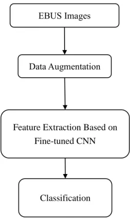
In this study, the EBUS diagnosis system based on the hybrid convolution neural network-support vector machine (CNN-SVM) classifier was proposed to differentiate between benign and malignant peripheral lung lesions. The proposed diagnosis system was composed of the sequential procedures including the data augmentation, the feature extraction based on the fine-tuned CNN and the lesion classification. To begin with, the data augmentation was performed to prevent the overfitting problem. Then, a convolutional neural network based on the fine-tuned CNN, CaffeNet, was utilized to extract features. After the feature extraction, the SVM classifier was trained based on the extracted features for distinguishing the benign lesions from malignant. The architecture of the proposed system was shown in Fig. 3-1.

(16)

Fig. 3-1. The architecture of the diagnosis system.

3.1. Data Augmentation

Because the deep neural networks were especially dependent on the availability of enormous quantities of training data for learning a non-linear function from input to output which yielded high classification accuracy on unseen data [26]. Therefore, for the smaller data, the data augmentation was utilized to enlarge the training data and

reduce the overfitting problem simultaneously [17]. In our study, the rotation and flipping image processes were applied on the EBUS images. However, because the difference of quantity between benign and malignant lesions might affect the

EBUS Images

Data Augmentation

Feature Extraction Based on Fine-tuned CNN

Classification

(17)

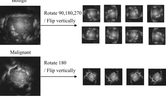
malignant cases were distinct. In malignant cases, the flipping with vertical axis and the rotation with 180 degrees image processes were performed. In benign cases, besides the vertical, and 180 degrees applied on the malignant cases, there were additional degrees, 90 and 270, used to rotate the images for shorten the difference of quantity between benign and malignant lesions. The results after flipping and rotation were shown in Fig. 3-2. This data augmentation produced eight modes of one benign case and four modes of one malignant case, respectively.

Fig. 3-2. Data augmentation.

3.2. Feature Extraction based on Fine-tuned CNN

Conventionally, a classification system is a time-consuming process when designing a feature extractor that transformed the raw data into feature vector as the input of a classifier. Recently, the deep learning model, CNN, allows feeding with raw

Benign

Malignant

Rotate 90,180,270 / Flip vertically

Rotate 180 / Flip vertically

(18)

data and automatically generating discriminative features for classification [13], it simplifies the process and reduces much time used to design a good feature extractor.

Therefore, the CNN was utilized in our proposed system. Because it was time- consuming to directly train a CNN from scratch, it could reduce the training time by fine-tuning a CNN that had been trained with a large dataset from a different application [27]. And the features extracted from the fine-tuned model were powerful for

classification [23]. Therefore, fine-tuning the model that transferred parameters from pre-trained model and extracting features from fine-tuned model were used in this study.

In following sections, the details of feature extraction including the layer functionality, the configuration in used CNN mode, the transfer learning, and the manner of feature extraction were described.

3.2.1. Convolutional Neural Network

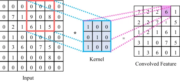
The convolutional neural network is a deep supervised learning structure and can be regarded as the architecture that constituted of an automatic feature extractor and a learnable classifier. The automatic feature extractor which retrieved features from the raw images was performed by two steps: the convolutional filtering and the down sampling. The convolutional filtering implemented with the weight sets regarded as kernels at convolutional layers was utilized to extract certain local features in the input images as shown in Fig. 3-3. In the convolutional layer, the value in each neuron

(19)

computed after the convolutional filtering was only relative to a small subset of the input images or the outputs of the layer. Furthermore, the neurons in the convolutional layers shared the same connection weights for controlling the number of weight throughout the input. After the convolutional filtering, the result of each filter was passed through a nonlinear activation function for approaching any function to improve the ability of CNN.

Fig. 3-3. The operation of convolution.

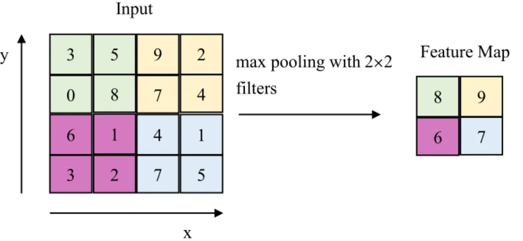
After performing the convolutional filtering, the down sampling operation was implemented in the pooling layer after each convolutional layer for reducing the computation complexity in the network. The most common down sampling operation was max pooling which applied a max filter to take the maximum feature value of the overlapping or non-overlapping sub-regions from the feature maps as shown in Fig. 3- 4. The convolutional and the pooling layers were the important characteristic of a CNN

0 0 7 2 0 0 1

3 0

0 0

1 9

6 1 0 0

0 6

0 0 0 8

5 1 0 0

5 7 0 1 0 0 0 8 0 0 0 0 0 0

0 0 0 0 0 0 0

0 1 0 1

0 1

0 0 0

2 7

2 2

2 1

6 2

7 ¹

6 1 3 1 0 7

1 3 6 0

1 5 1 5 1

*

=

Kernel

Input

Convolved Feature 0

(20)

which reduced the computation complexity than neural networks (NNs) [28]. Besides, another important characteristic was the automatic optimization of the weights in CNN performed by the backpropagation algorithm [13].

Fig. 3-4. The operation of max pooling.

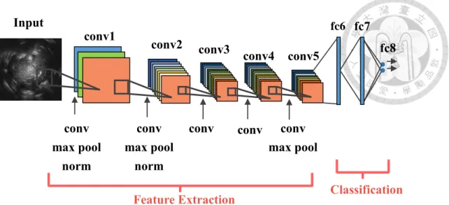
In this study, a higher performance CNN modified from AlexNet, the CaffeNet [29], was utilized for extracting the features. The CaffeNet contained five convolution and three fully-connected layers as shown in Fig. 3-5 and Table 3-1. The nonlinear activation function in the network was the Rectified Linear Unit (ReLU) which made the network train faster than using tanh or sigmoid function. The ReLU activation function is defined as following

f(x)= {x, x>0

0, x≤0 (1)

Then, because the purpose of this method was to deal with the classification of EBUS the number of outputs for the last fully-connected (FC) layer was replaced 1000 with 2.

5 3 0 8 6 1 3 2

2 9 7 4

1 4 7 5

x

y max pooling with2×2

filters

and stride 2

9 8 6 7 Input

Feature Map

(21)

Table 3-1. The configuration of the CaffeNet.

Layer Type Output size

data input 3×227×227

conv1 convolution 96×55×55 conv2 convolution 256×27×27 conv3 convolution 384×13×13 conv4 convolution 384×13×13 conv5 convolution 256×13×13 fc6 fully connected 4096×1×1 fc7 fully connected 4096×1×1 fc8 fully connected 2×1×1

conv5

fc6 fc7 conv3 conv4 fc8

conv2 conv1

Input

Feature Extraction Classification conv

max pool norm conv

max pool norm

conv conv conv

max pool

Fig. 3-5. The structure of the CaffeNet.

(22)

3.2.2. Fine-tuning the CNN

If the network were directly trained with scratch, the large number of weights in the layers would be randomly initialized. Therefore, the iterative updating of weights without a sufficient dataset might cause an unacceptable local minimum for the cost function. To overcome the problem, the fine-tuning based on the concept of transfer learning was performed in the proposed system. To begin with, the pre-trained model of CaffeNet which was previously trained on ImageNet [18]. Then, the weights of the pre-trained model were copied to the network which we want to train. Although the ImageNet and the EBUS images differ greatly, it was demonstrated that fine-tuning on the target data had potential for improving the performance [21]. After fine-tuning, the image features became more data-specific.

3.2.3. Feature Extraction

To achieve better performance than directly classifying with CNN, a method which was extracting features from the CNN model was utilized in this study. Moreover, the features were taken as training input for the SVM classifier. After fine-tuning the CaffeNet, the model could be seen as a feature extractor by taking the activations of one layer in CaffeNet. The higher layers generally produced discriminative features [30]

(23)

Therefore, the output of the fully connected layer 7 (fc7) was used as the features representation of EBUS images in this study. The features extracted from fc7 were a 4096-dimensional vector and the feature values were scaled by its maximum absolute value to the [-1, 1].

3.3. Classification

To differentiate benign and malignant lesions with better performance than directly classifying by the CNN, a supervised learning models, support vector machine (SVM), were utilized to classify the images with the training input from the features extracted from the layer of the model [25].

3.3.1. SVM

Support vector machine (SVM) [31] which was a supervised learning classifier was utilized to differentiate between benign and malignant images with the extracted features. The features from CaffeNet were included in the SVM model. Supposing a training set S={x_i,y_i}, where feature vector xi ∈ Rⁿ, and an indicator vector y ∈ R^l such that yi ∈{1,0} . The soft margin SVM tries to find a hyperplane that satisfies the following constrained optimization:

(24)

minω,b,ξ

1

2ω^Tω+C ∑ ξ_i

l

i=1

subject to y_i(ω^Tϕ(x_i)+b) ≥ 1 - ξ_i, ξ_i ≥ 0, i=1, . . . ,l,

where ω is a n-dimensional vector, b is a scalar, and C > 0 is the regularization parameter. There was a possibility that classification the EBUS images was a non-linear problem. To achieve better performance for the non-linear problem, the kernel function ϕ(x_i) was utilized to mapping feature vector xi into a higher dimensional space. In this study, the kernel function was the radial basis function kernel, also called the Radial Basis Function kernel. The SVM classifier produced the results which represented the probabilities of lesion tendency with range 0 to 1. And the threshold was set to 0.5. If the prediction probability exceeds 0.5, the sample is predicted to be malignant;

otherwise, benign.

(25)

Chapter 4 Experiment Results and Discussion

4.1. Experiment Environment

The experiments of the proposed computer-aided diagnosis (CAD) system included data augmentation, feature extraction based on fine-tuned CNN, classification.

All the methods were implemented by python programming language and python modules, such as numpy, opencv, scikit-learn and scikit-image which are always utilized in computer vision and machine learning. And the convolutional neural network used in the transfer learning was based on Caffe framework [32] which is developed by Berkeley AI Research (BAIR)/The Berkeley Vision and Learning Center (BVLC). The pre-trained models were from the Caffe Model Zoo [24]. The system was operated under the Microsoft Windows 10 operating system (Microsoft, Redmond, WA, USA) and ran on an Intel® Core™ i7-4790 3.6 GHz processor with 16GB RAM. And the transfer learning was ran on a Geforce GTX 1070 8GB GPU.

(26)

4.2. Results

The dataset containing 56 benign cases and 108 malignant cases was used to measure the performance of the experiments. To evaluate the performance of the CAD system, the five-fold cross validation method [33] was utilized. Six indicators included accuracy, sensitivity, specificity, positive predictive value (PPV), negative predictive value (NPV) and area under the curve (AUC) of receiver operating characteristic curve (ROC) were calculated. The ROC was obtained by using ROCKIT software (C. Metz;

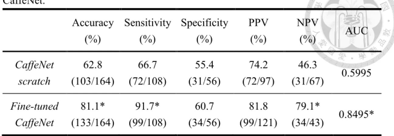
University of Chicago, Chicago, IL, USA). To examine whether using the pre-trained model was useful to improve the performance, the fine-tuned CaffeNet and the CaffeNet trained from scratch had a comparison and the results were shown in Table 4- 1. With the advantage of pre-trained model, the accuracy was improved from 62.8% to 81.1% and the sensitivity was increased from 66.7% to 91.7%. Moreover, their ROC curves were illustrated in Fig. 4-1. The diagnosis performance of the fine-tuned CaffeNet was statistically significant better than the CaffeNet directly trained from scratch with a p-value less than 0.05.

(27)

Table 4-1. The comparison between CaffeNet trained with scratch and fine-tuned CaffeNet.

Accuracy (%)

Sensitivity (%)

Specificity (%)

PPV (%)

NPV

(%) AUC

CaffeNet scratch

62.8 (103/164)

66.7 (72/108)

55.4 (31/56)

74.2 (72/97)

46.3

(31/67) 0.5995 Fine-tuned

CaffeNet

81.1*

(133/164)

91.7*

(99/108)

60.7 (34/56)

81.8 (99/121)

79.1*

(34/43) 0.8495*

The value with “*” means the p-value of the comparison between it and the first row< 0.05

Fig. 4-1. The ROC curve of the comparison of whether using pre-trained model.

0 0.1 0.2 0.3 0.4 0.5 0.6 0.7 0.8 0.9 1

0 0.2 0.4 0.6 0.8 1

True Position Fraction

False Position Fraction

ROC Curves

AUC=0.5995 CaffeNet scratch AUC=0.8495 Fine-tuned CaffeNet

(28)

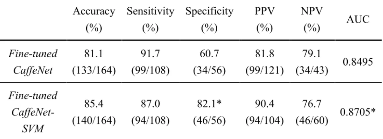
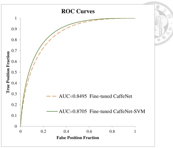
To determine whether the fusion of the fine-tuned CaffeNet and SVM have better performance, the fusion of the fine-tuned CaffeNet and SVM compared with the fine- tuned CaffeNet. Their results were listed in Table 4-2. The fusion of the fine-tuned CaffeNet and SVM boosted the specificity from 60.7% to 82.1% and the accuracy from 81.4% to 85.4%. The p-value of the AUC less than 0.05 indicated there was statistically

significant about the improvement. Their ROC curves were shown in Fig. 4-2.

Table 4-2. The comparison of whether classifying by SVM with the features from the fine-tuned CaffeNet.

Accuracy (%)

Sensitivity (%)

Specificity (%)

PPV (%)

NPV

(%) AUC

Fine-tuned CaffeNet

81.1 (133/164)

91.7 (99/108)

60.7 (34/56)

81.8 (99/121)

79.1

(34/43) 0.8495 Fine-tuned

CaffeNet- SVM

85.4 (140/164)

87.0 (94/108)

82.1*

(46/56)

90.4 (94/104)

76.7

(46/60) 0.8705*

(29)

Fig. 4-2. The ROC curve of the comparison of whether classifying by SVM with the features from Fine-tuned CaffeNet.

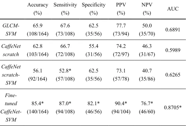
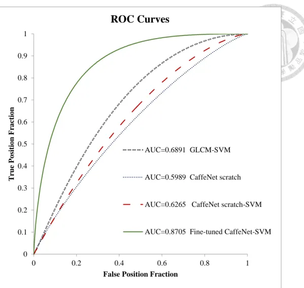
To evaluate whether the proposed CNN method was better than the conventional handcrafted approach, the gray-level co-occurrence matrix (GLCM) [34] method was performed in this experiment to extract second-order statistical texture features from EBUS images. Six GLCM features including contrast, correlation, homogeneity, energy, dissimilarity, ASM were utilized to classify with SVM. In Table 4-3, the results showed that the CaffeNet trained from scratch and the fusion of the CaffeNet trained from scratch and SVM was not superior to the handcrafted approach. Nevertheless, the

0 0.1 0.2 0.3 0.4 0.5 0.6 0.7 0.8 0.9 1

0 0.2 0.4 0.6 0.8 1

True Position Fraction

ROC Curves

AUC=0.8495 Fine-tuned CaffeNet AUC=0.8705 Fine-tuned CaffeNet-SVM

(30)

fusion of the fine-tuned CaffeNet and SVM outperformed the handcrafted method with statistical significance. Their ROC curves were illustrated in Fig. 4-3.

Table 4-3. The comparison between the handcrafted method and the CNN methods.

Accuracy (%)

Sensitivity (%)

Specificity (%)

PPV (%)

NPV

(%) AUC

GLCM- SVM

65.9 (108/164)

67.6 (73/108)

62.5 (35/56)

77.7 (73/94)

50.0

(35/70) 0.6891 CaffeNet

scratch

62.8 (103/164)

66.7 (72/108)

55.4 (31/56)

74.2 (72/97)

46.3

(31/67) 0.5989 CaffeNet

scratch- SVM

56.1 (92/164)

52.8*

(57/108)

62.5 (35/56)

73.1 (57/78)

40.7

(35/86) 0.6265 Fine-

tuned CaffeNet-

SVM

85.4*

(140/164)

87.0*

(94/108)

82.1*

(46/56)

90.4*

(94/104)

76.7*

(46/60) 0.8705*

(31)

Fig. 4-3. The ROC curve of the comparison between the handcrafted method and the CNN methods.

The other deeper neural networks including the VGGNet with 16 layers [35], the GoogleNet with 22 layers [36], the ResNet with 50 layers [37] were also utilized the transfer learning and the fine-tuning to examine whether the features from deeper neural networks with limited training data had better performance. In Table 4-4 the results showed the fusion of the fine-tuned CaffeNet with SVM was better than the fusion of the VGGNet with 16 layers, the GoogleNet, and the ResNet with 50 layers. And their ROC curves and training time were illustrated in Fig. 4-4 and listed in Table 4-5.

0 0.1 0.2 0.3 0.4 0.5 0.6 0.7 0.8 0.9 1

0 0.2 0.4 0.6 0.8 1

ROC Curves

AUC=0.6891 GLCM-SVM

AUC=0.5989 CaffeNet scratch

AUC=0.6265 CaffeNet scratch-SVM

AUC=0.8705 Fine-tuned CaffeNet-SVM

(32)

Table 4-4. The performance of the fusion of the fine-tuned CaffeNet and other deeper CNN models.

Accuracy (%)

Sensitivity (%)

Specificity (%)

PPV (%)

NPV

(%) AUC

Fine-tuned CaffeNet-

SVM

85.4 (140/164)

87.0 (94/108)

82.1 (46/56)

90.4 (94/104)

76.7

(46/60) 0.8705 Fine-tuned

VGG16- SVM

73.8*

(121/164)

81.5 (88/108)

58.9*

(33/56)

79.3*

(88/111)

62.3

(33/53) 0.7683*

Fine-tuned GoogleNet-

SVM

77.4 (127/164)

81.5 (88/108)

69.6 (39/56)

83.8 (88/105)

66.1

(39/59) 0.8337 Fine-tuned

ResNet50- SVM

73.8*

(121/164)

73.1*

(68/108)

75.0 (42/56)

84.9 (79/93)

59.2*

(42/71) 0.8394

(33)

Fig. 4-4. The ROC curve of the comparison between CaffeNet and other CNN models.

Table 4-5. The training time of the fusion of the fine-tuned CNN models and SVM.

Training Time (5 fold) Fine-tuned CaffeNet-SVM 3 minutes 40 seconds

Fine-tuned VGG16-SVM 50 minutes

Fine-tuned GoogleNet-SVM 15 minutes

Fine-tuned ResNet50-SVM 1 hour 27 minutes

0 0.1 0.2 0.3 0.4 0.5 0.6 0.7 0.8 0.9 1

0 0.2 0.4 0.6 0.8 1

ROC Curves

AUC=0.8705 Fine-tuned CaffeNet-SVM

AUC=0.8337 Fine-tuned GoogleNet-SVM

AUC=0.8394 Fine-tuned ResNet50-SVM

AUC=0.7683 Fine-tuned VGG16-SVM

(34)

4.3. Discussion

In this study, the fine-tuning based on the concept of the transfer learning was performed to overcome the problem of insufficient training data. The Table 4-1 showed that the fine-tuned CaffeNet initialized weights by the model trained with nature images successfully boosts the performance on classifying EBUS images which is not similar to nature images. Directly training with limited scratch was not sufficient to optimize the parameters of the CaffeNet; hence the performance was not good. As with the previous study [38], it was helpful to perform the transfer leaning from the large scale annotated nature image datasets (ImageNet). To achieve better performance, the fusion of the fine-tuned CaffeNet and SVM was performed in this study. In Table 4-2, the fusion of the fine-tuned CaffeNet and SVM improved the specificity and the performance. It represented that the features extracting from the fine-tuned CaffeNet was discriminative and the classification ability of SVM outperformed the direct classification with the CaffeNet using the softmax layer. The reason might be that the generalization ability of the SVM was better than that of the softmax layer [39].

Moreover, according to the experimental results shown in Table 4-3, the performance of the handcrafted method (GLCM+SVM) was higher than that of the CaffeNet directly trained with scratch but lower than the fine-tuned CaffeNet and the fusion of the

(35)

limited training data was not plenty to optimize the parameters of the CaffeNet; hence, the automatic feature extractor of the CaffeNet could not produce powerful features than the handcrafted method. Besides the CaffeNet, there have recently been many deeper networks proposed with better performance in the ImageNet Large Scale Visual Recognition Competition [40], like the VGGNet, the GoogleNet and the ResNet. In our experiments, the performance and the training time of the fusion of the fine-tuned CaffeNet and SVM which only contains 8 layers was better than the fusion with other fine-tuned deeper CNNs. The reason might be that the deeper neural networks with more parameters, hence they need more training data and training time to optimize.

Although the proposed system achieved higher performance, there were two limitations. First, the quantity of the original dataset was not sufficient for fine-tuning the model to achieve the performance as the expert diagnosis. Although the data augmentation was performed to expand the dataset, the distribution of the dataset was not enlarged too much. To overcome the limitation, it was necessary to acquire more labeled data for fine-tuning. Besides, the images of the dataset came from only the same type of machine. Therefore, it was unconfirmed whether the proposed system was robust to the images from different types of machines. There was a need to acquire the images from different types of machines for fine-tuning the model to confirm the

(36)

Chapter 5 Conclusion and Future Work

In this study, a CAD system classifying lung lesions into benign or malignant was proposed. The system utilized data augmentation to expand the size of training data.

Then feature extraction based on fine-tuned CNN was performed. It was achieved by initializing the CaffeNet with the weight pre-trained on ImageNet and then the layers were fine-tuned with scratch. Moreover, the features were extracted from the fully connected layer 7 of CaffeNet. Furthermore, the SVM model was applied with the features to differentiate between benign and malignant lesions. According to the experiment results, the accuracy, sensitivity, specificity, PPV, NPV and the AUC of this system achieved 85.4% (140/164), 87.0% (94/108), 82.1% (46/56), 90.4% (94/104), 76.6% (46/60) and 0.8705, respectively. The results showed that the fusion of the fine- tuned CaffeNet and SVM system had potential to assist detecting lung cancer. In addition, the proposed method outperformed than the conventional handcrafted method and was the first to utilize deep learning for diagnosing EBUS images automatically. It decreased the manual operation and the time for diagnosis. In the future, it was required to expand the data set with the same quantity of benign and malignant lesions to enhance the optimization of the model. In addition, there was a need to evaluate the

(37)

References

[1] R. L. Siegel, K. D. Miller, and A. Jemal, "Cancer statistics, 2016," CA: a cancer journal for clinicians, vol. 66, pp. 7-30, 2016.

[2] R. S. Fontana, D. R. Sanderson, W. F. Taylor, L. B. Woolner, W. E. Miller, J. R.

Muhm, et al., "Early Lung Cancer Detection: Results of the Initial (Prevalence) Radiologic and Cytologic Screening in the Mayo Clinic Study 1, 2," American Review of Respiratory Disease, vol. 130, pp. 561-565, 1984.

[3] T. N. L. S. T. R. Team, "Reduced Lung-Cancer Mortality with Low-Dose Computed Tomographic Screening," New England Journal of Medicine, vol.

365, pp. 395-409, 2011.

[4] M. Kaneko, K. Eguchi, H. Ohmatsu, R. Kakinuma, T. Naruke, K. Suemasu, et al., "Peripheral lung cancer: screening and detection with low-dose spiral CT versus radiography," Radiology, vol. 201, pp. 798-802, 1996.

[5] E. A. Kazerooni, F. T. Lim, A. Mikhail, and F. J. Martinez, "Risk of pneumothorax in CT-guided transthoracic needle aspiration biopsy of the lung,"

Radiology, vol. 198, pp. 371-375, 1996.

[6] T. Balamugesh and F. Herth, "Endobronchial ultrasound: A new innovation in bronchoscopy," Lung India: Official Organ of Indian Chest Society, vol. 26, p.

17, 2009.

[7] K. Yasufuku, T. Nakajima, M. Chiyo, Y. Sekine, K. Shibuya, and T. Fujisawa,

"Endobronchial ultrasonography: current status and future directions," Journal of Thoracic Oncology, vol. 2, pp. 970-979, 2007.

[8] H. Wada, T. Nakajima, K. Yasufuku, T. Fujiwara, S. Yoshida, M. Suzuki, et al.,

"Lymph node staging by endobronchial ultrasound-guided transbronchial needle aspiration in patients with small cell lung cancer," The Annals of thoracic surgery, vol. 90, pp. 229-234, 2010.

[9] T.-Y. Chao, C.-H. Lie, Y.-H. Chung, J.-L. Wang, Y.-H. Wang, and M.-C. Lin,

"Differentiating peripheral pulmonary lesions based on images of endobronchial ultrasonography," CHEST Journal, vol. 130, pp. 1191-1197, 2006.

[10] C.-H. Lie, T.-Y. Chao, Y.-H. Chung, J.-L. Wang, Y.-H. Wang, and M.-C. Lin,

"New image characteristics in endobronchial ultrasonography for differentiating peripheral pulmonary lesions," Ultrasound in medicine &

biology, vol. 35, pp. 376-381, 2009.

[11] P. Nguyen, F. Bashirzadeh, J. Hundloe, O. Salvado, N. Dowson, R. Ware, et al.,

"Grey scale texture analysis of endobronchial ultrasound mini probe images for

(38)

2015.

[12] K. Fukushima and S. Miyake, "Neocognitron: A self-organizing neural network model for a mechanism of visual pattern recognition," in Competition and cooperation in neural nets, ed: Springer, 1982, pp. 267-285.

[13] Y. LeCun, Y. Bengio, and G. Hinton, "Deep learning," Nature, vol. 521, pp. 436- 444, 2015.

[14] Y. LeCun, L. Bottou, Y. Bengio, and P. Haffner, "Gradient-based learning applied to document recognition," Proceedings of the IEEE, vol. 86, pp. 2278- 2324, 1998.

[15] C.-K. Shie, C.-H. Chuang, C.-N. Chou, M.-H. Wu, and E. Y. Chang, "Transfer representation learning for medical image analysis," in Engineering in Medicine and Biology Society (EMBC), 2015 37th Annual International Conference of the IEEE, 2015, pp. 711-714.

[16] J.-Z. Cheng, D. Ni, Y.-H. Chou, J. Qin, C.-M. Tiu, Y.-C. Chang, et al.,

"Computer-aided diagnosis with deep learning architecture: applications to breast lesions in US images and pulmonary nodules in CT scans," Scientific reports, vol. 6, p. 24454, 2016.

[17] A. Krizhevsky, I. Sutskever, and G. E. Hinton, "Imagenet classification with deep convolutional neural networks," in Advances in neural information processing systems, 2012, pp. 1097-1105.

[18] J. Deng, W. Dong, R. Socher, L.-J. Li, K. Li, and L. Fei-Fei, "Imagenet: A large- scale hierarchical image database," in Computer Vision and Pattern Recognition, 2009. CVPR 2009. IEEE Conference on, 2009, pp. 248-255.

[19] Y. Bar, I. Diamant, L. Wolf, and H. Greenspan, "Deep learning with non-medical training used for chest pathology identification," in Proc. SPIE, 2015, p. 94140V.

[20] H.-C. Shin, H. R. Roth, M. Gao, L. Lu, Z. Xu, I. Nogues, et al., "Deep convolutional neural networks for computer-aided detection: CNN architectures, dataset characteristics and transfer learning," IEEE transactions on medical imaging, vol. 35, pp. 1285-1298, 2016.

[21] R. Girshick, J. Donahue, T. Darrell, and J. Malik, "Rich feature hierarchies for accurate object detection and semantic segmentation," in Proceedings of the IEEE conference on computer vision and pattern recognition, 2014, pp. 580- 587.

[22] P. Sermanet, D. Eigen, X. Zhang, M. Mathieu, R. Fergus, and Y. LeCun,

"Overfeat: Integrated recognition, localization and detection using convolutional networks," arXiv preprint arXiv:1312.6229, 2013.

[23] A. Sharif Razavian, H. Azizpour, J. Sullivan, and S. Carlsson, "CNN features

(39)

IEEE conference on computer vision and pattern recognition workshops, 2014, pp. 806-813.

[24] C. Cortes and V. Vapnik, "Support-vector networks," Machine learning, vol. 20, pp. 273-297, 1995.

[25] B. Athiwaratkun and K. Kang, "Feature representation in convolutional neural networks," arXiv preprint arXiv:1507.02313, 2015.

[26] J. Salamon and J. P. Bello, "Deep convolutional neural networks and data augmentation for environmental sound classification," IEEE Signal Processing Letters, vol. 24, pp. 279-283, 2017.

[27] N. Tajbakhsh, J. Y. Shin, S. R. Gurudu, R. T. Hurst, C. B. Kendall, M. B. Gotway, et al., "Convolutional neural networks for medical image analysis: Full training or fine tuning?," IEEE transactions on medical imaging, vol. 35, pp. 1299-1312, 2016.

[28] J. Schmidhuber, "Deep learning in neural networks: An overview," Neural networks, vol. 61, pp. 85-117, 2015.

[29] J. Donahue, "Caffenet," ed, 2016.

[30] M. D. Zeiler and R. Fergus, "Visualizing and understanding convolutional networks," in European conference on computer vision, 2014, pp. 818-833.

[31] V. Vapnik, The nature of statistical learning theory: Springer science & business media, 2013.

[32] Y. Jia, E. Shelhamer, J. Donahue, S. Karayev, J. Long, R. Girshick, et al., "Caffe:

Convolutional architecture for fast feature embedding," in Proceedings of the 22nd ACM international conference on Multimedia, 2014, pp. 675-678.

[33] R. Kohavi, "A study of cross-validation and bootstrap for accuracy estimation and model selection," in Ijcai, 1995, pp. 1137-1145.

[34] R. M. Haralick and K. Shanmugam, "Textural features for image classification,"

IEEE Transactions on systems, man, and cybernetics, pp. 610-621, 1973.

[35] K. Simonyan and A. Zisserman, "Very deep convolutional networks for large- scale image recognition," arXiv preprint arXiv:1409.1556, 2014.

[36] C. Szegedy, W. Liu, Y. Jia, P. Sermanet, S. Reed, D. Anguelov, et al., "Going deeper with convolutions," in Proceedings of the IEEE conference on computer vision and pattern recognition, 2015, pp. 1-9.

[37] K. He, X. Zhang, S. Ren, and J. Sun, "Deep residual learning for image recognition," in Proceedings of the IEEE conference on computer vision and pattern recognition, 2016, pp. 770-778.

[38] H. C. Shin, H. R. Roth, M. Gao, L. Lu, Z. Xu, I. Nogues, et al., "Deep Convolutional Neural Networks for Computer-Aided Detection: CNN

(40)

Transactions on Medical Imaging, vol. 35, pp. 1285-1298, 2016.

[39] D.-X. Xue, R. Zhang, H. Feng, and Y.-L. Wang, "CNN-SVM for microvascular morphological type recognition with data augmentation," Journal of Medical and Biological Engineering, vol. 36, pp. 755-764, 2016.

[40] O. Russakovsky, J. Deng, H. Su, J. Krause, S. Satheesh, S. Ma, et al., "Imagenet large scale visual recognition challenge," International Journal of Computer Vision, vol. 115, pp. 211-252, 2015.