美國西南部地區上部地幔震波層析成像

(1)

國立臺灣大學理學院地質科學研究所碩士論文

Department of Geosciences College of Science

National Taiwan University Master Thesis

美國西南部地區上部地幔震波層析成像

Multi-Scale Finite-Frequency Travel-time Tomography Applied to Imaging 3-D Velocity Structure of the Upper Mantle beneath the Southwest United States

尹一帆 Yin, Yi-Fan

指導教授﹕洪淑蕙博士中華民國九十八年一月

January 2009

(2)

(3)

Abstract

Seismic tomography has played a key component in unraveling the deep processes that caused the surface morphology and rift magmatism in the southwest United States.

Earlier study used teleseismic body-wave arrivals recorded by the La Ristra experiment, a dense broadband array of 950-km in length deployed during 1999-2001 and run through the Great Plains, the Rio Grande Rift (RGR), and the Colorado Plateau, to construct a 2-D tomographic image of the upper mantle structure beneath this linear array. However, because of the inevitable smoothing and damping imposed in the inversion, the resulting velocity contrast is too weak to explain distinct P and S waveform changes across the array. In this study, all the available data from the La Ristra, nearby arrays, and newly deployed USArray are utilized for the determination of frequency-dependent travel-time shifts by inter-station cross correlation of waveforms at both high- (0.3-2 Hz for P and 0.1-0.5 Hz for S) and low-frequencies (0.03-0.125 Hz for P and 0.03-0.1 Hz for S).

Different from the previous models that rely on classical ray theory and regular grid parameterization, the new tomographic images are built based on state-of-the-art 3-D, finite-frequency sensitivity kernels that relate observed travel-time data to velocity heterogeneity and a wavelet-based, multi-scale parameterization that enables to yield robust structures with spatially-varying resolutions subject to data sampling. The resulting P and S models reveal a prominent smile-shaped region of low wave speed anomalies encircling the Colorado Plateau and confined in the uppermost 250 km depth.

The lowest velocity anomalies are highly correlated with the late Cenozoic volcanic fields but do not underlie the rift center. At depths greater than 250 km, the variations of P and S velocity structures appear less coherent with the surface geological features. A very slow-velocity core inside the Colorado Plateau extending from ~300 km to greater depths may provide a plausible explanation for its elevated topography.

Key Words: tomography, United States, finite frequency, multi-scale, wavelet

(4)

摘要

震波層析成像是瞭解地球深部之動力機制的重要工具，在研究美國西南部地質及構造的研究中為其深部的動力解釋提供重要證據。其中，從 1999 至 2001 年，

長 950 公里、橫跨 Colorado Plateau、Rio Grande Rift 及 Great Plains 的 La Ristra 線性陣列在此設立，希望能觀測穿過此三個不同地質區的地幔剖面。利用前述資料所建構的二維模型由於在逆推速度構造時無法避免的正則化與平滑化問題，其所解出之速度異常幅度太小，無法解釋 P 波及 S 波沿著陣列觀測到的波形變化。

本研究利用 La Ristra 陣列和附近所有能取得的資料，結合新近設立的 USArray 地震觀測網得到更完整的資料覆蓋。P 波及 S 波走時資料經濾波成高低兩個頻帶(高頻：P 波 0.3-2 Hz，S 波 0.1-0.5；低頻：P 波 0.03-0.125 Hz，S 波 0.03-0.1 Hz)，

並利用波形間互相比對求得最佳化的走時異常。不同於傳統的震波層析成像採用波線理論與格點參數化，本研究使用有線頻寬理論以及以小波理論為基礎的多尺度參數化來建構其速度模型。有線頻寬理論能更真實的反應三圍速度構造與走時異常的對應，多尺度參數化則使模型能隨資料密度自行調整解析度。

反演結果顯示由 50 公里深度直到 250 公里處，速度異常分佈大致與地表地質構造相關。最明顯的為環繞 Colorado Plateau 南部，並隨晚新生代火山帶延伸向東的慢速構造。250 公里以下，速度構造與地表地質構造的關聯漸消失。在 Colorado Plateau 下方，300 公里以下有明顯慢速構造存在，此一慢速異常可能為高原的海拔高度提供浮力來源。

關鍵字：美國、層析成像、多尺度、有限頻寬、小波

(5)

List of Figures

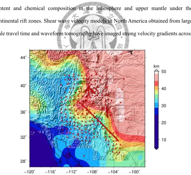
Fig. 1-1. (a) is the topographic map of the southwestern United States. Stations used in this study are denoted by triangles with various colors that stand for different networks labeled on the bottom of (b) ... 2 Fig. 1-2. Variations of the crustal thickness under the southwestern United States. .... 3 Fig. 1-3. 2-D P- and S-wave velocity models of the upper mantle under the La Ristra

array derived from body-wave travel time tomography [[Gao et al., 2004] ... 5 Fig. 1-4. 2-D shear velocity structurel of the crust (top panel) and upper mantle down

to ~400 km depth (bottom panel) under the La Ristra array derived from surface wave inversion [West et al., 2004]. ... 5 Fig. 1-5. Topographic variations of upper mantle seismic discontinuities from P-to-S

conversions revealed from receiver function migration images. ... 6 Fig. 1-6. Finite-difference synthetic waveform modeling using the S-wave model of

Gao et al. [2004].. ... 6 Fig. 2-1. Geographical distribution of all the events used in the study.. ... 14 Fig. 2-2. Illustration of frequency-depdent travel-time residuals and waveforms.. ... 20 Fig. 2-3. Lateral variations of relative travel time shifts determined from

high-frequency P waves ... 21 Fig. 3-1. The ray plane cross-sectional views of the Born-Fréchet kernels of P, PcP,

PKPdf, S, and ScS phases, respectively, used in this study. ... 29 Fig. 3-2 Topographic map of the study area and grid discretization denoted by gray

lines used for model parameterization. ... 38 Fig.3-3. Comparison between (a) ray-theoretical sensitivity and (b) finite-frequency

kernel sensitivity from high frequency P, PcP, and PKPdf travel-time data.. ... 39 Fig. 3-3 (Continued) Comparison between (c) ray-theoretical sensitivity and (d)

finite-frequency kernel sensitivity from low frequency S and ScS travel-time data..

... 40 Fig. 3-3 (Continued) Finite-frequency sensitivity for P+PcP+PKPdf and S+ScS data

including all the data measured at both high- and low-frequency bands. ... 41 Fig. 3-4. Tradeoff curves of variance reduction versus model variance (left) and

variance reduction versus model norm (right) ... 42 Fig. 3-5. Tradeoff curves of variance reduction versus model variance (left) and

variance reduction versus model norm (right) for S and ScS dataset.t. ... 43 Fig. 4-1. Tomographic images of P-wave velocity perturbation for the (a) ray

(7)

viewed on three vertical cross sections (middle column) and six constant-depth maps (two right columns) from 94 km to 531 km depth... 49 Fig. 4-2. Tomographic images of S-wave velocity perturbation for the (a)

ray-theoretical and (b) finite frequency models. ... 50 Fig. 4-3. Resolution tests for the P-wave models using available path coverage of the

observed travel-time data. The input model shown in (c) has an alternating checkerboard pattern of positive and negative velocity perturbations, ±2% with eight grid sizes, ~248 km wide in each side. ... 51 Fig. 4-4. Resolution tests for the S-wave models using available path coverage of the

observed travel-time data. The input checkerboard model is the same as in Fig.

4-3. ... 52 Fig. 4-5. Resolution tests for the P-wave models using available path coverage of the

observed travel-time data. Each checkerboard occupies six grid sizes, ~186 km wide on each side.. ... 53 Fig. 4-6. Resolution tests for the S-wave models using available path coverage of the

observed travel-time data. Each checkerboard occupies six grid sizes, ~186 km wide on each side.. ... 55 Fig. 4-7. Resolution tests for the P-wave models using available path coverage of the

observed travel-time data. Each checkerboard occupies four grid sizes, ~124 km wide on each side.. ... 56 Fig. 4-8. Resolution tests for the S-wave models using available path coverage of the

observed travel-time data. Each checkerboard occupies four grid sizes, ~124 km wide on each side.. ... 57 Fig 5-1. Tomographic images of P- and S-wave velocity anomaly beneath CD-ROM

transect.. ... 60 Fig 5-2. Finite-frequency P-wave tomography of southwestern U. S.. ... 60

List of Tables

Table.1. List of seismic networks and numbers of available broadband stations used in the study……….………...12 Table. 2. Frequency bands used for P- and S-wave travel-time measurements…...…15 Table. 3. Ranges of epicentral distances of the events used for measurements of

various types of phase arrivals………...…………..15 Table. 4. Numbers of relative travel-time shifts of various phases measured at high-

and low-frequency bands…………..………18

(8)

1 Introduction

The vast and complicated landscape of western North America has been attributed to the long history of the ancient Farallon plate that began subducting underneath it about 70 Ma ago. Orogenies, volcano activities, and accompanying uplift and extension shaped the continent into different units of distinct tectonic features as seen today.

The Rio Grande Rift (RGR), one of the largest-scale topographic manifestations in the southwestern United States, extends approximately north-southwardly from the south tip of Rocky Mountains in Colorado, runs through New Mexico, gradually merges with Basin and Range Province in Chihuahua, Mexico and terminates in the westernmost part of Texas [Keller and Baldridge, 1999]. It is surrounded by the Rocky Mountains to the north, the Great Plains to the east, the Colorado Plateau to the west and the Basin and Range Province to the south and southeast (Fig. 1-1).

The opening of the RGR system started about 35 Ma ago when the crust and mantle lithosphere were pulled apart by the regional extension, inducing the upwelling of asthenospheric mantle to replace the thinning lithosphere and generate melts by pressure release melting. The upper crust have undergone brittle failure and formed a series of asymmetrical half grabens [Wilson et al., 2005]. Though being relatively dormant today, intensive igneous extrusion and volcanic activities have taken place during the rift-initiation period [Humphreys, 1995]. Heat flow measurements in the RGR show higher values than the surrounding Great Plains and Colorado Plateau [Slack et al., 1996].

In addition, the crustal thickness across the rift varies dramatically from on average 44.1 km under the Great Plain to about 35 km under the rift axis [Olsen et al., 1987; Wilson et al., 2005] (Fig. 1-2). The most recent volcanic activities occurred to the west of the main

(9)

(a)

(b)

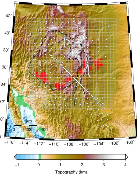
Fig. 1-1. (a) is the topographic map of the southwestern United States. GP: Great Plains; RM: Rocky Mountains; CP: Colorado Plateau; BR: Basin and Range Province. Black lines outlined the Rio Grande Rift. Dashed line circles the Colorado Plateau. Red-shaded regions mark the late Cenozoic volcanic fields with the average ages less than 4.5 million years old. Stations used in this study are denoted by triangles with various colors that stand for different networks labeled on the bottom of (b). Geological features shown on the map are modified from [Spence and Gross, 1990].

(10)

fields, spanning about 800 km long and running from the Rayton Clayton volcanic field, northeastern New Mexico to the San Carlos volcanic field, Arizona, mark the transition zone between Colorado Plateau and Rio Grande Rift and obliquely intersect the rift axis [Spence and Gross, 1990] (Fig. 1-1).

Numerous geological and geophysical investigations have been conducted in this region, aiming at understanding the tectonic mechanism that influences the evolution and structure of continental rifts [Perry et al., 1988; Spence and Gross, 1990; Baldridge et al., 1991; Slack et al., 1996; Gao et al., 2004; Song and Helmberger, 2007]. Seismic tomographic imaging has been a useful tool to reveal underlying seismic velocity and attenuation structures, which provide important clues on the temperature, melt/fluid content and chemical composition in the lithosphere and upper mantle under the continental rift zones. Shear wave velocity models in North America obtained from large scale travel time and waveform tomography have imaged strong velocity gradients across

Fig. 1-2. Variations of the crustal thickness under the southwestern United States based on the

(11)

the margin of the stable cratonic keel and high wave speed anomalies in the upper mantle beneath the western United States associated with the remnants of the subducted Farallon plate [Grand, 1994; Lee and Nolet, 1997]. In the past two decades, the increasing temporary deployment of dense seismic arrays across continents has improved the tomographic images with unprecedented resolutions [Spence and Gross, 1990;

Humphreys and Dueker, 1994; Slack et al., 1996].

Different rifting mechanisms, either pure-shear or simple-shear deformation, result in distinguishable symmetric or asymmetric configuration of the crust and mantle lithospheric structure [Olsen et al., 1987; Wilson et al., 2005]. In order to construct the high-resolution seismic images of upper mantle velocity structure and topographic variation on the crust-mantle interface under the RGR, a NW-SE trending linear array of about 950 km long that consists of 54 broadband instruments spaced, on average, 18 km apart was deployed across the rift from July 1999 to May 2001. The Colorado PLAteau/Rio Grande Rift Seismic TRAnsect Experiment (hereafter referred as La Ristra and coded as XM in Fig. 1-1), with its two ends running through the Colorado Plateau and the Great Plains, was designed to record teleseismic wave arrivals from abundant earthquakes in the Aleutian and South American subduction zones which directly probe the crust and upper mantle beneath these three tectonic regions [Wilson et al., 2003].

The data collected by the La Ristra array have been thoroughly explored in various seismological studies including body-wave and surface-wave travel time tomography [Gao et al., 2004; West et al., 2004; Wilson et al., 2005], shear wave splitting analysis [Gök et al., 2003], and receiver function imaging [Wilson et al., 2003; Wilson et al., 2005].

[Gao et al., 2004] present the 2-D, ray-based P- and S-wave models which yield the largest amplitude variations within the upper 200 km depth (Fig. 1-3). The slow

(12)

anomalies lie beneath the rift axis and become more deeply rooted under the closely-linked Jemez Lineament. Between the volcanic lineament and the Colorado Plateau exists a sharp velocity boundary. Under the eastern plateau shows a high velocity region, whereas beneath the central part resolves a significant low velocity zone extending from the surface to ~300 km depth which might contribute to the once active Navajo volcanic field at around 20-30 Ma ago. Further west to the verge, the fast anomaly,

Fig. 1-3. 2-D P- and S-wave velocity models of the upper mantle under the La Ristra array derived from body-wave travel time tomography [[Gao et al., 2004]

Fig. 1-4. 2-D shear velocity structurel of the crust (top panel) and upper mantle down to

~400 km depth (bottom panel) under the La Ristra array derived from surface wave inversion [West et al., 2004].

(13)

eastern end of the array the fast anomalies are imaged under the Great Plains at the depths above 200 km and between 300 km and 600 km in S-wave model. This sheet-like feature is interpreted as the downwelling limb associated with the small-scale convection. (Fig.

1-3)

Shear velocity structure imaged from surface wave dispersion reveals a broader low velocity zone in the uppermost mantle above 150 km depth beneath the rift axis [West et al., 2004]. It extends laterally about 150-200 km on both sides of the rift axis, ends abruptly under the Great Plains to the east, and gradually merges with deeper slow regions at depths greater than 150 km under the Colorado Plateau to the west. The rather

Fig. 1-5. Topographic variations of upper mantle seismic discontinuities from P-to-S conversions revealed from receiver function migration images [Wilson et al., 2003].

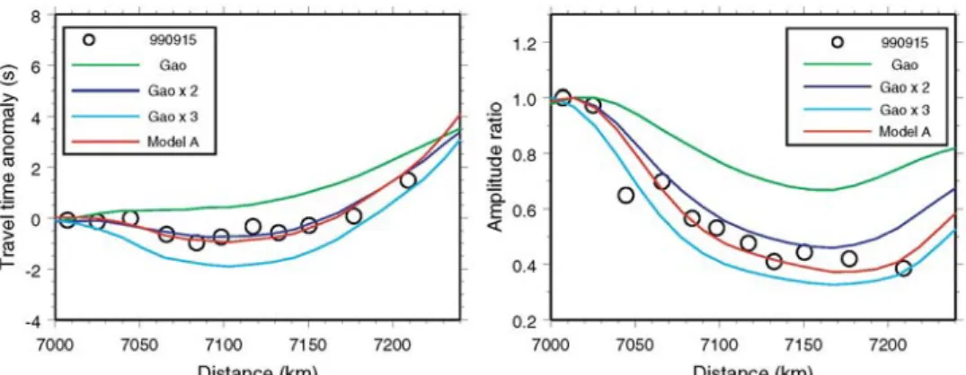
Fig. 1-6. Finite-difference synthetic waveform modeling using the S-wave model of Gao et al. [2004]. The model is amplified by one, two and three times to meet the actual observation of travel time anomalies and amplitude ratio. Model A is constructed by amplifying the fast anomaly by 2 and slow anomaly by 4 in order to get better fit. [Song and Helmberger, 2007]

(14)

warm mantle under the plateau from ~150 to 275 km depth has been interpreted as the asthenosphere which replaced the falling Farallon slab and was capable of providing the buoyancy needed to support the average 1.8 km elevation of the Colorado Plateau. The low velocity anomaly under the Rio Grande Rift does not appear to be fed by a deeper source, suggesting that the rift might be passively driven by the lithospheric extension [West et al., 2004]. The receiver function imaging from [Wilson et al., 2003] also shows negligible topographic variations on the 410 km and 670 km seismic discontinuity, indicating there is no localized thermal anomaly in the transition zone under the region. It thus concludes that the major thermal signature is predominantly confined to the uppermost mantle above 400 km depth (Fig. 1-5). Besides, the topography of the Moho discontinuity shows a 10 km rift-symmetric crustal thinning beneath the rift, suggesting a pure shear thinning mechanism which is also supported by surface wave results.

Because of the lack of low velocity anomaly extending down to the deeper transition zone and lower mantle [Gao et al., 2004; Wilson et al., 2005], the integrated seismic evidences support the scenario in which small-scale convection occurred in response to the lithospheric extension and thinning. Moreover, an elongated, relatively high wave speed feature was detected at the margin of well-resolved regions, which has been attributed to the fragment of the subducted Farallon slab [Gao et al., 2004].

[Song and Helmberger, 2007] employed 2-D finite-difference waveform modeling to calculate synthetic P and S waveforms in 2-D heterogeneous velocity structures beneath the La Ristra array resolved from previous tomographic studies. The predicted travel time and amplitude variations of P and S waves across the array were too weak to match the observed results, suggesting that either the regularization invoked to suppress the noisy short-wavelength fluctuations has sacrificed the power spectra of the tomographic models or finite-frequency effects on observed travel time delays was not properly taken

(15)

into account in classical ray-based tomography. Stronger velocity heterogeneity by increasing a factor of 2 for fast anomaly and 4 for slow anomaly yields significantly improved fits of observed travel time and amplitude anomalies (Fig. 1-6).

To account for intrinsic wavefront healing effects on finite-frequency seismic waves, the tenet of seismic tomography has moved on from ray theory in the infinite frequency limit to physically-realistic finite-frequency theory [Dahlen et al., 2000]. Considering the destructive interference of scattered waves from velocity heterogeneities at different frequencies, the travel time shift of a finite frequency phase arrival is no longer sensitive to seismic wave speed perturbations along its infinitesimally narrow ray path; rather, it is mostly influenced by 3-D volumetric structure surrounding the path. Whenever the scale length of heterogeneity is on the order of the cross path width of the sensitivity zone that depends on the dominant wavelength and propagation distance of the wave, finite-frequency wavefront healing becomes significant and ray theory will overestimate observed travel time anomalies and thus underestimate the strength of velocity heterogeneity. Benefiting from the great leap in computing power and the availability of high-quality data from dense broadband seismic networks, finite-frequency theory has been extensively employed to better resolve the images of upwelling mantle plumes [Hung et al., 2004; Montelli et al., 2004] and fine scale structures in the lowermost mantle [Hung et al., 2005].

Alternatively, due to uneven data coverage, data uncertainty and approximation of forward theory, different model parameterization and regularization schemes imposed on the tomographic inversion can lead to the non-uniqueness of the resolved velocity model.

Multiscale model construction through the wavelet decomposition and synthesis was then introduced to better achieve the spatial resolution in densely-sampled regions while securing the long-wavelength spectral resolution [Chiao and Kuo, 2001; Chiao and Liang,

(16)

2003]. The merit of the multiscale tomography lies on the automatic determination of the tomographic images with spatially varying, data-adaptive resolvable scales.

In this study, all the important elements in seismic travel time tomography, including frequency-dependent travel-time observations, finite-frequency theory, and multi-resolution parameterization are essentially combined to reconstruct 3-D high-resolution images of P and S velocity perturbations beneath the southwestern United States. The region of interest spans from 28° to 42° in latitude and -114° to -100° in longitude. All the accessible teleseismic data recorded from the permanent and temporary broadband stations distributed in the area are collected through Data Management Center (DMC) of Incorporated Research Institutions for Seismology (IRIS). In addition to data from the linear La Ristra array and a few stations nearby to the east deployed in early 90s, 170 available USArray stations covering the west of the study region are also incorporated in this study. As a part of the ambitious NSF-funded EarthScope Project, the USArray has been underway since the fiscal year of 2005 and planned to sweep the entire United States starting from the west coast with 400 neatly pinned transportable seismometers of 50-70 km spacing over a 10-year period. Using seismic waves as probes, the experiment is aimed at investigating the structure and dynamics of the continental lithosphere under North America and the earth’s deep interior. The IRIS DMC provides the timely and open data access, which substantially augments the dataset used in this study.

I reexamine finite-frequency travel time shifts measured by inter-station cross correlation of waveforms band-pass filtered at high- (0.3-2 Hz for P and 0.1-0.5 Hz for S waves) and low-frequency bands (0.03-0.125 Hz for P and 0.03-0.1 Hz for S waves).

Employing more accurate finite-frequency sensitivity kernels for relative travel-time measurements and the wavelet-based multi-scale parameterization in the inversion, I

(17)

anticipate to yield more robust 3-D lithospheric and upper mantle structures under the RRGR and adjacent regions and gain more insights into the regional tectonics and mantle dynamics that characterize the surface geology and underlying velocity structure.

(18)

2 Data

2.1 Data processing

Regional travel-time tomography relies on the observations of travel-time variations of P and S waves from distant earthquakes across an array of seismograph stations densely deployed in the area of interest. Therefore, I searched all the available broadband stations located in the study region, which is centered at the RGR and ranges from 28°N to 42°N in latitude and 100°W to 114°W in longitude. The waveform data recorded globally at teleseismic distances, i.e., epicentral distance greater than 30^o, with magnitudes >= 5.5 were then retrieved from Data Management Center (DMC) of the Incorporated Research Institutions for Seismology (IRIS) by means of a handy JAVA-based SOD (Standard Order for Data) program. The SOD program is a very useful tool in seismology developed by the University of South Carolina and designed to automatically select, download, and routinely process massive seismic data which match the user-defined criteria specified by earthquake parameter, station distribution or a combination of both [Owens et al., 2004]. For the events that occurred prior to the year of 2001, the origin times and hypocenter locations were based on the relocated ISC (International Seismological Centre) catalog by [Engdahl et al., 1998]. For those recent events occurring in 2007 and 2008, the earthquake information was obtained from the Monthly Hypocenter Data File (MHDF) and Weekly Hypocenter Data File (WHDF) distributed by National Earthquake Information Center (NEIC) at the US Geological Survey (USGS).

Table 1 compiles a number of permanent and temporary seismic networks spanning over the last three decades which provide broadband stations and data used for the

(19)

tomographic study. It is noted that the station coverage is much denser on the western half of the study region due to the timely schedule of the USArray transporting to the Colorado Plateau during the years of 2007 and 2008 (figure 1-1).

Network Description Time span #station

TA USArray 2007-2008 170

XM La Ristra 1999-2001 58

XK CDROM 1999-2000 34

XL Deep Probe 1997 32

XG Rocky Mountain Front 1992 26

US United States National Seismic Network 1991 ~ 9

IW Intermountain West 2004 ~ 3

IM TXAR Array 1970~ 2

NR NARS Array 1983 ~ 2

IU Global Seismograph Network 1988 ~ 2

UU University of Utah Regional Network 1981 ~ 1

Table.1 List of seismic networks and numbers of available broadband stations used in the study.

Because the instruments of earlier seismic experiments before 2001 were equipped with various types of broadband sensors (STS-2, CMG-3T, CMG-3ESP, and CMG-40T), they would yield considerably different responses for a velocity impulse input, particularly in the pulse tails that accordingly had influences on estimated travel time residuals by waveform cross correlation. Therefore, prior to cross-correlation travel time measurements, the instrument responses of the raw seismograms were equalized by removing their individual instrument responses and convolving the resulting waveforms with the CMG-40T sensor response.

In order to measure relative travel-time anomalies of various body-wave phases between stations, including P, PcP, PKPdf, S and ScS waves used to constrain the variations of P and S wave speeds in the upper mantle beneath the RGR, I first subtracted the arrival times of individual phases predicted from a radially-symmetric Earth model,

(20)

AK135 for the continental velocity structure [Kennett et al., 1995]. The seismograms were then windowed 80 s before to 200 s after the expected phase arrivals and applied with a fourth-order, zero-phase Butterworth band-pass filter.

The travel time of an actually band-limited seismic wave measured by a waveform cross correlation method is explicitly frequency dependent, because the lower frequency wave ‘feels’ the structure farther off the ray path and experiences larger degree of wavefront healing while the higher frequency wave is more sensitive to small-scale structures close to the ray [Hung et al., 2001; Yang and Hung, 2005]. Such frequency-dependent characteristics are well represented by 3-D finite-frequency sensitivity kernels which make it tenable to jointly invert travel-time data measured at multiple frequency bands, each of which contributes complementary knowledge to the heterogeneous velocity structure of the earth’s interior. I thus chose to measure the travel-time anomalies of P- and S-wave phase arrivals in both high- and low-frequency ranges using the first complete cycles of the band-pass filtered waveforms on the vertical and transverse component, respectively. As the P- and S-wave signals usually comprise different frequency contents, the bandwidths selected for P and S waves are not the same in order to suppress the noise level and highlight the signals suitable for cross correlation travel-time measurements. The cutoff frequencies of the high- and low-frequency band-pass filters applied to P and S phase arrivals are listed in Table 2.

Moreover, to avoid the potential contamination of multiple phases arriving closely within the cross correlation time windows, the events used for measuring various types of phase arrivals are limited to certain ranges of epicentral distances within which only the desired single phase is expected to emerge according to the travel-time curves predicted by the 1-D reference Earth model (see Table 3).

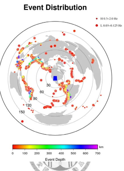
Fig. 2-1 displays the distributions of azimuths and epicentral distances of 1196

(21)

earthquakes in high-frequency data and 1045 earthquakes in low-frequency data that provide the travel-time data for the tomographic imaging of P and S velocity structures.

The majority of the useful events occurring along the circum-Pacific seismogenic belt are concentrated in the azimuth range counterclockwise from northwest to southeast, while the events in the Eurasian and African continents toward the opposite azimuths are rather scarce. The uneven geographical distribution of data is commonly a natural defect for the passive tomographic imaging such that the regularization will come into play in the inversion to solve for the physically-reliable velocity models intrinsically with spatially-varying resolutions.

Fig. 2-1. Geographical distribution of all the events used in the study. Large circles denote the events for the measurement of low-frequency travel time data; small circles denote those for high-frequency data.

(22)

Phase High frequency (Hz) Low frequency (Hz)

P 0.3 – 2.0 0.03 – 0.125

S 0.1 – 0.5 0.02 – 0.2

Table. 2 Frequency bands used for P- and S-wave travel-time measurements.

P wave S wave

P 30 – 99.3 S 30 – 80

PKPdf 120 - 180 ScS 50 - 75

PcP 30 - 70

Table. 3 Ranges of epicentral distances of the events used for measurements of various types of phase arrivals.

2.2 Cross correlation travel-time measurements

[VanDecar and Crosson, 1990] pointed out that the waveforms from teleseismic events recorded by the regional arrays or networks with closely-spaced stations (about 10-20 km apart) remain coherent suitable for the determination of relative travel-time shifts (residuals) between stations by a waveform cross correlation method. The travel-time residual between a pair of stations is objectively determined by finding a time shift to make their waveforms most similar and yield a maximum cross correlation.

For the arrays with larger station spacings and wide apertures, the phase arrivals affected by the multipathing and scattering through 3-D velocity heterogeneity appear to be nearly random and the resulting waveforms may not be coherently similar across the stations. The distorted waveforms are thus considered as random errors added to the phase pulses used for cross correlation travel-time measurements. They introduced a multi-channel cross-correlation (MCCC) method to simultaneously determine the optimal relative travel-time shifts of individual stations and estimate the uncertainties of the resulting travel-time residuals. Rather than choosing the waveform of a master

(23)

station as a reference pulse to be cross-correlated with those from the rest of stations, the MCCC technique first determines the cross-correlation time shifts between all the station pairs. It then uses these measured time shifts as data to set up an over-determined system of linear equations. The unknowns corresponding to the optimal relative travel-time residual for each station are therefore calculated from a least squares solution with their uncertainties estimated from the root-mean-square (RMS) errors between the cross-correlation measured residuals and predicted results of all the station pairs.

For all the recorded traces from one single event, the discrete form of cross-correlation function, ^Φ^ij

( )

^τ , as a function of time shift, τ, between the ith and jth trace is given by [VanDecar and Crosson, 1990],

( )

^/ ⁰ ⁰

1

( ) ( )

T t

p p

ij i i j j

k

t s t t k t s t t k t

T δ δ

τ δ τ δ

=

= + + + ⋅ + +

Φ

∑

^, ⁽¹⁾

where si and sj are the waveform traces in the cross-correlation time windows of length T recorded at the ith and jth station, respectively; tip and tjp represent the theoretical arrival times predicted by the spherically-symmetric AK135 model, t0 is the time difference between the starting time of the correlation window and predicted arrival times, and δt the sampling interval of traces. The window length T is approximately scaled to the dominant periods of the cross-correlation waveforms. The relative travel-time shift, Δt_ij, between the ith and jth station derived from waveform cross correlation is thus expressed as

Δt_ij = − −t_i^p t^p_j τ_ij^max^, ⁽²⁾

where τ_ij^max corresponds to the time lag at which the ^Φ^ij

( )

^τ^ij^max reaches the maximum value.

With all the measured relative travel-time shifts between any pair in a total of N

(24)

stations, an over-determined system of N(N-1)/2 linear equations is formed by t_i _{− = Δ}t_j t_ij, where i=1,…, N-1, and j=i+1,…, N. (3)

While solving the N unknowns of ti, i=1,…,N, corresponding to the optimized relative travel-time residual of each station, an extra constraint that forces the mean of relative travel time shifts for each event to be zero is usually applied in the inversion by adding the equation,

1 N

0

i i

t

=

∑

^. ⁽⁴⁾

The least squares solution for ti‘s is obtained from minimizing the root-mean-square misfits between the cross-correlation derived residuals, Δt_ij, and the residual difference,

(t_i −t_j), calculated from the solutions,

²

, 1,

min ^N _ij, where _ij _ij ( _i _j)

i j i j

res res t t t

= ≠

= Δ − −

∑ ^. ⁽⁵⁾

The error for the resulting ti of each station can be assessed from the standard deviation σⁱ of the misfits, res_ij,

2 , 1,

1 ^N

i ij

i j i j

σ res

γ = ≠

= ∑

, (6)

where γ is the degree of freedom used to estimate the travel-time measurement error.

As each individual misfit res_ijis considered not be completely independent from the others, γ is chosen to be N-2 as suggested by [VanDecar and Crosson, 1990].

The travel-time measurements were conducted through a semi-automatic procedure which provides an interactive window to carefully inspect and eliminate the seismograms with inaccurate clocks or uncorrelated pulse shapes prior to the waveform cross correlation. Besides, the cycle-skipping problems encountered while finding the

(25)

cross-correlation maximum were fixed by adjusting the cross-correlation time windows or removing the traces with unreasonably large time shifts.

2.3 Variations of relative travel-time shifts

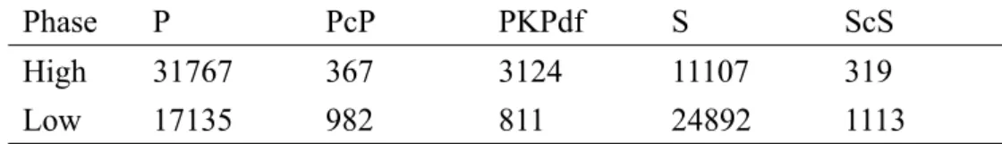
Table 4 summarizes the total numbers of relative travel-time residuals measured in two frequency bands for various kinds of the P and S phases.

Phase P PcP PKPdf S ScS

High 31767 367 3124 11107 319

Low 17135 982 811 24892 1113

Table. 4 Numbers of relative travel-time shifts of various phases measured at high- and low-frequency bands.

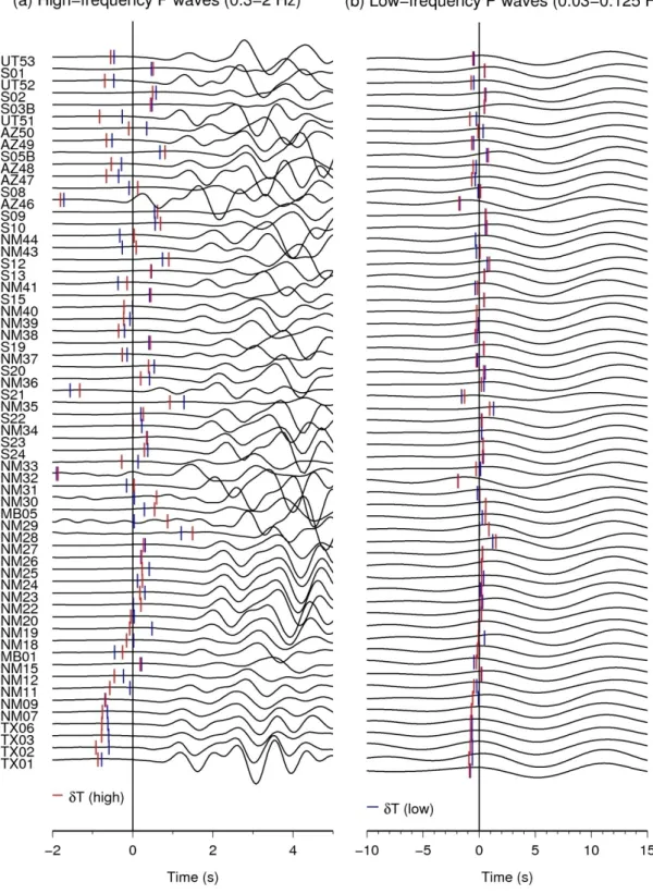
Provided that the travel-time anomaly of a finite-frequency seismic wave was accrued solely from the velocity perturbations along its geometrical ray path, the cross-correlation travel-time residuals measured in different frequency bands would be invariant. Comparing the variations of the relative travel-time residuals obtained from high- and low-frequency waveforms across the stations as shown in Fig. 2-2, the magnitudes of the high-frequency residuals are in general larger than the low-frequency ones. This suggests that the seismic wave of different frequencies actually samples different volumetric velocity structures and travels with different wave speeds which results in the frequency-varying time residuals. The most sensitivity volume of a phase arrival is approximately confined within the first Fresnel zone surrounding the ray path associated with the region where the constructive interference of different frequency seismic waves takes place [Wielandt, 1981]. The lateral extent of the first Fresnel zone grows proportionally to the square root of the dominant wavelength of a seismic wave times the propagation distance to the station. Whenever the scale length

(26)

of 3-D velocity heterogeneity is on the order of the lateral width of the sensitivity zone of the traveling wave, the wavefront healing phenomenon caused by wave diffraction around a slow or fast velocity anomaly becomes prominent and the accrued travel-time delay or advance is gradually diminished as time progresses. As a consequence the lower-frequency waves will undergo more significant wavefront healing and lead to smaller travel-time shifts than the higher-frequency waves.

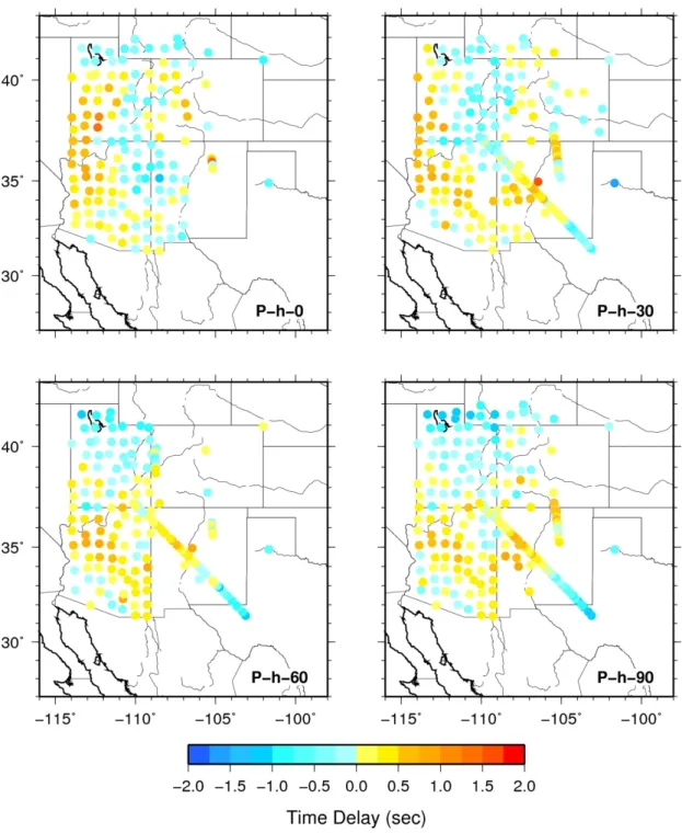
In Fig. 2-3, the variations of the relative travel-time shifts measured from high-frequency P phase arrivals are displayed to shed some light on the lateral variation of the underlying P-wave velocity structure. The events are binned into groups over a series of backazimuth swaths with every 30-degree increments. For each group, the average travel-time shift of each station plotted on the map is calculated by the mean of all the measured travel-time shifts weighted inversely proportional to their respective measurement errors. Most maps delineate the distinctly separate regions of positive and negative travel-time residuals. Overall, the stations with positive residuals corresponding to relatively slow P arrivals form a smile-shaped area encircling the core of the Colorado Plateau. The stations situated in the center of the Colorado Plateau, the Great Plains and the Basin and Range Province yield negative residuals associated with relatively fast P arrivals. The events from the north (-30°~30°) generally give negative time residuals in the areas coincident with the Colorado Plateau and the Rocky Mountains. Whereas the events from the rest of azimuths show a large area of positive residuals spreading throughout the entire plateau, leaving the area of negative residuals confined within the Rocky Mountains and the Great Plains. As such, the azimuthal dependence of relative travel-time residuals suggests that there exists the 3-D heterogeneous structure with distinct velocity contrasts under the study area which needs further verification in the tomographic inversion.

(27)

Fig. 2-2. Illustration of frequency-depdent travel-time residuals and waveforms. As a result of diffractive wavefront healing, the residuals measured from waveforms in the high frequencies, marked with red ticks, in general have larger amplitudes than those measured in the low frequencies as denoted by blue ticks.

(28)

Fig. 2-3. Lateral variations of relative travel time shifts determined from high-frequency P waves.

The value for each station is obtained from the weighted average of the travel time shifts from the events with their back azimuths within ±¹⁵^o ranges from the back azimuths indicated on the lowerleft corner of each map.

(29)

Fig. 2-3 (Continued)

(30)

Fig. 2-3 (Continued)

(31)

3 Method

3.1 Forward Theory and Data Rule

3.1.1 Linearized Ray Theory

According to the high-frequency asymptotic approximation of the elastodynamic wave equation, propagation of seismic wave fields through the heterogeneous Earth can be constructed from the sum of a bundle of rays, each of which travels along its infinitely-thin ray path between a source and receiver for which the travel time remains stationary, akin to Fermat’s principle in optics. The information carried by the arrival times (and amplitudes) of various body-wave phases directly reflects the local elastic properties along their individual ray paths and is readily applicable to tomographic imaging of seismic velocity structure where these rays pass through.

In a smoothly-varying and slightly-perturbed heterogeneous medium, Fermat’

principle dictates that the travel-time shift due to the deviation of the ray path is of second order and negligible, compared to that owing to the velocity perturbation itself [Dahlen et al., 2000]. Such approximation leads to linearized ray theory most commonly used in conventional travel-time tomography. Therefore, the travel-time shift, δt, of a seismic phase relative to the predicted arrival in a 1-D reference Earth model is simply calculated by the integral of the slowness (reciprocal of velocity) perturbation along the unperturbed ray path [Dahlen et al., 2000],

^δ

^t ⁼∫_ray^δ

(

^{1 ( )}^{c x dl}

)

^, ⁽¹⁾

where dl is the incremental arc length, c(x) the wave speed at point x along the unperturbed ray in the 1-D model, and ^δ

( )

^{1 c} the slowness perturbation to be imaged.

(32)

3.1.2 Banana-Doughnut Theory

Ray theory is strictly valid only in the limit of the infinite frequency. In reality, the spectra of seismic waves and responses of recorded seismograph instruments are both finite. The inherent limitation of high-frequency rays fails to account for the contributions of wavefront healing, scattering and other finite-frequency diffraction effects around the structural heterogeneity off the ray paths to observed seismic wave arrivals. In other words, the travel-time shift measured from a broadband seismic phase actually detects the 3-D velocity structure surrounding its geometrical great-circle path. As the resolvable scale length of the tomographic images has been steadily improved by more available high-quality, broadband seismic data and approaches close to the characteristic width of the Fresnel zone for the observed phase arrival, differences between the actual finite-frequency travel-time shifts and corresponding ray-theoretical predictions become essentially important [Hung et al., 2001; Baig et al., 2003]. As a result, they need to be taken into account in the forward formulation of the Fréchet kernels that relate measured finite-frequency travel-time data to 3-D velocity structure to be imaged in tomography.

Recent development in finite-frequency kernel theory, or referred as to banana-doughnut theory, based on Born single-scattering approximation has founded the theoretical underpinnings of finite-frequency travel-time tomography [Marquering et al., 1999; Dahlen et al., 2000; Zhao et al., 2000]. Considering the destructive interference between waves of different frequencies through a heterogeneity point, the sensitivity of the derived Fréchet kernel lies farther off the ray path, depending on the power spectrum of the cross-correlation waveforms that gives rise to frequency-dependent travel-time shifts. The 1-D line integral in equation (1) is then replaced by the 3-D volumetric

(33)

integration of the derived kernel over the earth’s interior with nonzero lateral velocity perturbations [Dahlen et al., 2000],

δ

t =∫∫∫_⊕K x c x c x d x( ) ( ) / ( )δ ³ ^. ⁽²⁾

The quantity K(x) is the 3-D Born-Fréchet kernel for a travel-time shift measured by cross correlation of an observed phase arrival and the corresponding 1-D synthetics.

Since only the waves forward-scattered off the velocity heterogeneity inside the first Fresnel zone and taking the same type of detoured routes as the unscattered direct wave will arrive closely together within the time window of a half period of the wave and have a significant contribution to the measured travel-time shift, [Dahlen et al., 2000]

employed a paraxial forward-scattering approximation to efficiently reduce the computational cost of calculating a 3-D kernel. The paraxial kernel K(x) is then expressed as [Dahlen et al., 2000],

3 2 0

2 2 0

( ) sin( ) 1

2 ' " ( )

( )

r

s T d

c c s d

K x ω ω ω ω

π ω ω ω

∞

⎛ ℜ ⎞ Δ

⎜ ⎟

⎝ ℜ ℜ ⎠

= − ∫

∫ _{, (3)}

where ΔT is the additional travel time required by the wave taking a detoured path through a point scatterer at x, i.e., the integration point x with fractional velocity perturbation, δc c/ , in equation (2). The scaling constants c and cr respectively correspond to the wave speed at the scatterer x and receiver r in the 1-D reference model, and R, R’ and R” stand for the geometrical spreading factors for the unperturbed ray, the forward source-to-scatterer ray, and the backward receiver-to-scatterer ray, respectively.

The additional travel times and geometrical spreading of the detoured scattered waves as required for the kernel computation is determined by dynamic ray tracing assuming a parabolic wavefront curvature in the vicinity of the paraxial (unperturbed) ray. s( )ω is ² the power spectrum of the finite-bandwidth waveform of a seismic phase used in cross

(34)

correlation travel-time measurement which explicitly specifies the frequency-dependent nature of the obtained travel-time shift.

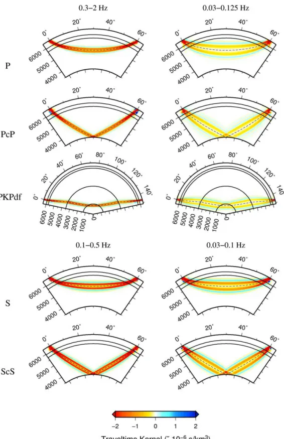
Figure 3-1 displays the 3-D Fréchet sensitivity kernels of high- and low-frequency measured travel-time shifts relative to the arrival times predicted by the AK135 model for a variety of phases including P, S, PcP, ScS, and PKPdf, plotted on the great-circle ray-plane cross sections. Except for the PKPdf travel-time kernel shown at an epicentral distance of 147°, all the other kernels are computed at a distance of 60°. All the kernels more or less retain the banana-doughnut shapes that exhibit the maximum sensitivity in the banana skin surrounding the doughnut hole with very weak sensitivity [Hung et al., 2000; 2001]. A finite-frequency travel-time shift yields zero sensitivity to a point scatterer of velocity perturbation right on the ray path, as seen in equation (3) where the additional detour time ΔT readily drops to zero. This is essentially contradictory to the interpretation of ray theory which attributes the observed travel-time shift to the velocity heterogeneity along the ray. The banana skin with the negative value of sensitivity that gives rise to a positive travel-time shift owing to a slow velocity anomaly is usually referred as to the Fresnel zone with the cross-path width proportional to (λL)^1/2, where λ is the characteristic wavelength of a seismic phase arrival and L is the propagation distance to the receiver [Hung et al., 2001]. The higher the frequency content of the wave is, the narrower the finite-frequency kernel for the measured travel-time shift is. As the frequency of a seismic wave goes to infinity, the 3-D kernel simply reduces to the 1-D linearized ray.

While long-period waves traveling through relatively small-scale heterogeneity, linearized ray theory is no longer a valid approximation and the use of the 3-D kernels becomes indispensable for accurately imaging the geometry and amplitude of the target structure. For the differential travel-time data such as the relative travel-time shifts between stations used in regional teleseismic tomography, the differential kernel is

(35)

obtained simply by the difference of the individual Fréchet kernels between two stations, i.e.,

K_{δ δ}t1₋ t2 ₌K_δt1 ₋K_δt2. (4)

(36)

Fig. 3-1. From top to bottom rows shows the ray plane cross-sectional views of the Born-Fréchet kernels of P, PcP, PKPdf, S, and ScS phases, respectively, used in this study. Two different frequency bands are chosen for cross-correlation measurements of P- and S-waves arrivals: 0.3-2 Hz and 0.03-0.125 Hz for P and 0.1-0.5 Hz and 0.03-0.1 Hz for S. The maximum sensitivity of each phase arrival shown in red colors appears in the first side lobe akin to the banana skin surrounding the ray as denoted by dashed lines. The cross-sectional diameter of the banana-shaped kernel is proportional to the square root of the propagation distance times the dominant wavelength of the wave. As a result, the lower-frequency travel-time kernels on the right column have broader sensitivity zones, whereas the higher-frequency kernels on the left shrink tightly to the ray. Overall, the sensitivity of a finite-frequency travel-time shift is exactly zero right on the

(37)

3.2 Model Parameterization and Regularization

3.2.1 Grid Parameterization

Various fields of scientific inverse problems, including seismic tomographic imaging, invoke the use of a finite amount of discrete data to solve for an unknown continuous model. The general data rule for the inverse problem can be expressed as [Chiao and Kuo, 2001; Chiao and Liang, 2003],

( ) ( ) 3

i Dgi m d ei

d ₌∫ ^x ^x ^x₊ ^, ⁽⁵⁾

where di is the ith travel-time data with its error ei, for i=1,…, N, x the position vector in a 3-D vector model space, D, and _i( ) ( ) ³ ( ( ), ( ))_i

Dg m d = g m

∫ ^x ^x ^x ^x x represents the inner product within the Hilbert space [Parker, 1977]. The data kernel, gi(x), is the Fréchet derivative of a functional that maps the continuous model function m(x) into the discrete data di. For my tomographic study, the pursued model is the variation of fractional velocity perturbations of the crust and upper mantle beneath stations constrained with observed relative travel-time shifts between pairs of the stations. Compared with the 1-D ray-theoretical integral as described in equation (1), the model to be solved for is just the slowness (inverse of velocity, c) perturbation, δ(1/c), and the data kernel gi(x) simply corresponds to the differential ray-path length, dl, of two phase arrivals for a measured relative travel-time shift. If banana-doughnut theory in equation (2) is instead adopted to assess the relationship between data and model, then gi(x) is related to the difference of the 3-D integration of the finite-frequency kernels between two phase arrivals within an infinitesimal volume, i.e. Kd³x.

For regional seismic tomography, the model function of the continuous variation of seismic velocity perturbations is conventionally expanded in term of a set of local basis functions, ( )φ_l x , orthonormal to each other with the truncation level L, where

(38)

( ( ), ( ))φ_i x φ_j x =δ_ij, and i, j=1,…,L [Chiao and Liang, 2003],

1

( ) ^L _{l l}( )

l

m β φ

=

∑

x x . (6)

Presumably that the grid discretization of the model space is fine enough, the errors in (6) from the truncated expansion up to the level L can be neglected. With the model of velocity perturbations specified at grid nodes and the spatial delta functions as basis functions, the discrete data rule used to invert for the expansion coefficient β_l equivalently to the velocity perturbations m at the lth node is thus written as [Chiao and _l Liang, 2003],

1 1

( ( ), ( ))

L L

i i l l il l

l l

g x A m

d _φ _β

= =

=

∑

^x =

∑

^, ⁽⁷⁾

where di is the ith relative travel-time shift data, and ml the mode parameter of fractional velocity perturbation at the lth node. If the tomography is based on ray theory, Ail is the difference of the summed ray path lengths between two phase arrivals through a specific volume or voxel that contributes to the lth node from the ith-paired relative travel time measurement. While finite frequency theory is instead invoked, Ail becomes the differential value of the integrated volumetric kernels, Kd³x , contributing to the lth node.

Numerical integration of the kernel value of a single voxel is obtained by the weighted sum of 27 sampling points according to the Gaussian quadrature formula [Zienkiewicz and Taylor, 1989]. Equation (7) can be further recast into a concise matrix form,

d=Am, (8)

where d is the data vector comprising a total of N measured relative travel-time shifts, [δt1, δt2,…,δtN]^T, equal to the inner product of the N × L Gram matrix A of Fréchet derivatives and the model vector of dimension L, m=[m1, m2,…,mL]^T.

(39)

3.2.2 Regularization

The tomographic inverse problems always encounters the defective conditions that arise from the uneven data sampling owing to geographical distribution of earthquakes and stations, finite amount of error-embedded data, finite parameterization of the continuous model, and implicit approximation of forward theory. As a result, some model parameters are well-determined but others poorly-constrained, particularly for those unsampled models that cause the null space problem and nonuniqueness of the model solutions. Besides, the small singular values of the Gram matrix that would produce large model variances and unstable solutions have to be exclusively removed or damped to effectively reduce their influence on the inverted model. Therefore, regularization is inevitably invoked in the inversion to select one preferred model among many possible solutions.

In the following, I will briefly summarize the regularization methods applied to assess the optimal model in the study. The most commonly-used regularization for the underdetermined inverse problem is the weighted, damped least squares (DLS) method which attempts to constrain a minimum-norm model [Menke, 1989],

mˆ =(A C A^T ⁻¹ +θ²I)⁻¹A C d , ^T ⁻¹ (9)

where I is an L×L identity matrix, and C the N×N data covariance matrix defined as

2

σi

=

C I, where σ_iis the estimated error for the ith data assuming each measure is independent. θ² is a nonnegative damping factor specified prior to the inversion to provide the intended harshness of the minimum norm criterion. The approximate inverse of the massive, sparse matrix is usually solved by the iterative LSQR algorithm [Paige and Saunders, 1982].

The under-parameterization of the continuous model with finite and coarse grid

(40)

discretization would lead to spectral leakage and aliasing [Trampert and Snieder, 1996;

Chiao and Kuo, 2001]. The over-parameterization is thereby suggested in travel-time tomography, though the nature of unevenly-distributed rays often leaves a large portion of the unsampled model parameters and the others redundantly sampled by similar ray paths.

The minimum-norm damping suppresses overall the amplitudes of the resolved velocity model; meanwhile, it sacrifices the spectral resolution of the better-constrained long-wavelength feature in the model. The alternative regularization scheme is combined with the convolution quelling which ad hoc broadens the cross-path width of rays and penalizes the model roughness by imposing an a priori correlation length of the model [Chiao and Liang, 2003],

mˆ =W W( ^T^{A C AW}^T ⁻¹ +θ²^I)⁻¹^{W A C d}^T ^T ⁻¹ , (10) where W is the convolution operator that prescribes a stationary correlation length on the resolved model [Meyerholtz et al., 1989]. If W is an identity matrix, equation (10) reduces to the weighted DLS solution in (9). The convolutional quelling solution acts similar as the “fat ray” approach which accounts for the finite-frequency sensitivity of broadband travel-time data but not for the wavefront healing effect.

Both the above two approaches regularize the degrees of model smoothness and length isotropically throughout the model space. Since the data sampling is not uniform, the spatial and spectral resolutions essentially vary from region to region. The stationary smoothing is thus inappropriate, especially for the densely-sampled region potentially with higher resolutions. A number of multiscale parameterizations have been introduced to cope with the heterogeneous data sampling and multi-resolution model. One of them is the use of nonuniform grids [Bijwaard et al., 1998]; the other is based on the natural hierarchical structure of the wavelet transform [Chiao and Kuo, 2001; Chiao and Liang, 2003].

(41)

signal processing, function approximation and image compression. By means of the discrete wavelet transform (DWT) using the discretely sampled wavelets, a digital signal can be level-by-level decomposed into one globally-averaged part and the other locally-detailed part on successive scale levels. The process is easily reversed by performing the level-wise synthesis of the detailed and the averaged parts.

Rewrite the data rule in equation (6) as a vector form,

d_i ₌ A m_il _l _{= ⋅m}a_i , (11)

where m corresponds to the model vector consisting of the L fractional velocity perturbations at grid nodes, and ai represents the ith row of the Gram matrix A. Let W(m) be the multi-dimensional wavelet transform of m. Introducing the biorthogonal wavelet bases, the dual and inverse wavelet transform functions, W^* and W^-1, respectively, associated with W, the biorthogonality relation between W^* and W^-1 renders equation (11) to be recast in a form,

d_i = ⋅a W_i ⁻¹W(m)=W a W^*( )_i ⋅ ( )m =W a^*( )_i ⋅m_MR, (12) where W^*(ai) denotes the wavelet transform of a particular row of the matrix A using the dual wavelet basis functions, and mMR the multiscale-parameterized model. Without the need to recalculate the matrix of Fréchet derivatives for mMR, equation (2) simply performs the wavelet transform of the original matrix A built on simple grid parameterization. The multiscale inversion imposes the minimum-norm damping regularization on the transformed Gram matrix, W^*(ai), and solves for the wavelet representation of the model. Finally, the model m parameterized at grid nodes is reconstructed from the inverse wavelet transform of mMR,

mˆ =W⁻¹(^m_MR). (13)

The inverse wavelet transform can be executed on the models summed up to any level, allowing us to inspect the spatial changes of the models and the associated improvements

(42)

in the model resolution and data fit on different scale levels.

3.3 Model Setting and Data Sampling

The study area is parameterized into 33×33×33 nodes with the horizontal spacing of about 36.26 km and vertical spacing of 31.25 km. The model space centered at the Rio Grande Rift laterally expands the area enclosing all the stations used, and vertically extends from the surface down to the depth of 1000 km (Fig. 3-2).

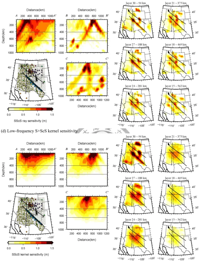
To assess the spatial distribution of the data sampling from the different perspectives of ray theory and finite-frequency theory, the diagonal values of the product of the transpose of the Gram matrix A^T and A, i.e., diag(A^TA), are calculated as a measure of sampling density. Each element of diag(A^TA) represents the total sum of the squares of the path lengths of 1-D rays or of the square values of 3-D volumetric kernels that contribute to a certain node. The velocity variations at the nodes with dense crossing rays or large amplitudes of sensitivity kernels implicitly have the potential to be better resolved.

Fig. 3-3 presents the three vertical cross sections and six constant-depth maps of the diag(A^TA) values in a logarithm scale. The area of the highest sensitivity is under the La Ristra array along which the stations were densely deployed and served for the longest period. For the ray-theoretical sensitivity plot, the ray-path trajectories are clearly seen, especially for those received by the La Ristra array. The very narrow sensitivity primarily confined along the ray path results in heavily fragmented images as observed in Fig. 3-3(a) and (c). Other than the La Ristra array, the USArray with the deployment of evenly-spaced stations provides fairly uniform sensitivity above 400 km depth. Below 400 km remains only intense ray beams received by the La Ristra array.

On the other hand, the sampling of finite-frequency kernels is relatively more

(43)

homogeneous because of their banana-doughnut shapes and broad cross-path widths.

For the sensitivity plot including only the high-frequency travel-time data, the sampling distribution is more or less similar to that depicted by ray theory as shown in Fig. 3-3(b).

Whereas combined with the sensitivity from the low frequency data, the differences immediately come into sight in Fig. 3-3(d). The regions where no rays even travel through can be yet “felted” by the off-path sensitivity of the finite-frequency waves passing nearby.

There is no standard criterion to compare the models based on different data rules.

Moreover, for a family of the resolved models evoked with different regularization parameters, there always exists a tradeoff between data fitness and model complexity.

Therefore, the typical tradeoff analysis between data fit and model norm or variance is conducted to choose the optimal model. The model goodness of fit to observed data is evaluated by variance reduction, VR, calculated from

2

1 2 1

( ˆ)

1 100%

N

i i

i N

i i

d d

VR

d

=

⎡ ⎤

⎢ − ⎥

= −⎢ ⎥×

⎢ ⎥

⎣ ⎦

∑

∑ ^, ⁽¹⁴⁾

where di is the ith travel-time shift, and ˆd the corresponding prediction from the _i chosen model. Figs 3-4 and 3-5 show the tradeoff relations for the resolved P and S models, respectively. The tradeoff curves between variance reduction and model variance associated with different forward theory and parameterization invoked in the inversion are shown on the left, while those between variance reduction and model norm are shown on the right. The comparisons of three parameterization methods including the damped least square (simple), multi-scale, and horizontal multi-scale and vertical convoluting quelling hybrid parameterization are made in (a) and (b) of these two figures. Regardless of the invoked data rule or forward theory, multi-scale parameterization always achieves the highest degree of variance reduction whereas the