K.-T. Lee et al. (Eds.): MMM 2011, Part I, LNCS 6523, pp. 193–205, 2011.
© Springer-Verlag Berlin Heidelberg 2011
for Versatile 3D Vision Applications and Its Automatic Adaptation to Imprecise Camera Setups
Shen-En Shih1 and Wen-Hsiang Tsai1,2
1 Institute of Computer Science and Engineering, National Chiao Tung University, Taiwan [email protected]
2 Department of Information Communication, Asia University, Taiwan [email protected]
Abstract. A new two-omni-camera system for 3D vision applications and a method for adaptation of the system to imprecise camera setups are proposed in this study. First, an efficient scheme for calibration of several omni-camera pa- rameters using a set of analytic formulas is proposed. Also proposed is a tech- nique to adapt the system to imprecise camera configuration setups for in-field 3D feature point data computation. The adaptation is accomplished by the use of a line feature of the console table boundary. Finally, analytic formulas for computing 3D feature point data after adaptation are derived. Good experimen- tal results are shown to prove the feasibility and correctness of the proposed method.
Keywords: omni-directional camera, camera calibration, adaptation to impre- cise camera setups, 3D data computation, computer vision applications.
1 Introduction
With the advance of technologies, various types of omni-directional cameras have been used for many applications, like virtual and augmented reality, TV games, video surveillance, 3D environment modeling, etc. In order to interact with human beings, most applications require acquisition of 3D data of feature points. This usually means in turn the need of a precise camera setup to yield accurate 3D data computation re- sults. However, from the viewpoint of a non-technical user, it is not reasonable to ask him/her to set up the cameras at right places and orient them to right directions with- out errors. Therefore, the system should be designed to have a capability to adapt to camera setup errors automatically.
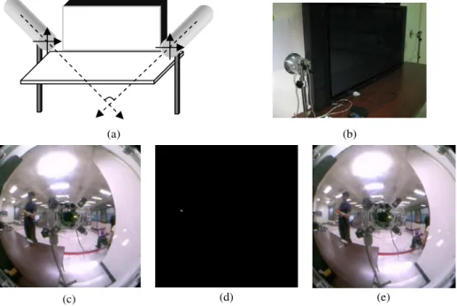
In this study, we first propose a novel method to calibrate omni-cameras, which is more efficient than traditional methods. Next, we propose a new 3D vision platform for various applications, as shown in Fig. 1, which consists of two omni-cameras, a console table, and a display (see Fig. 1(a) for an illustration). Each camera is affixed to the top of a rod, forming an “omni-camera stand.” The two stands are placed beside the console table, which is located in front of the display (see Fig. 1(b)). The display may be a TV, a large monitor, a projection screen, etc. The height of the rod of each
omni-camera stand is adjustable to fit the height of the console table and/or that of the user of the system. While placing the omni-camera stands beside the table, the cam- eras are supposed to be oriented exactly forward to face the user and used to take omni-images of the user’s activity in front of the table (see Fig. 1(c)). The two cam- eras are assumed to be well calibrated in the factory by the proposed calibration method, and the optical axes of the two omni-cameras are supposed to be mutually parallel and both horizontal with respect to the floor. If the omni-camera stands are set up precisely in this way in the field, then the 3D data computation can be conducted precisely as well. As an example of applications of the proposed system for 3D data computation, Fig. 1(c) shows the case of a user using a finger tip of his, covered with a yellow cot, as a 3D cursor point, which is useful for 3D space exploration in video games, virtual or augmented reality, 3D graphic designs, and so on. Fig. 1(d) shows the extracted finger tip region and Fig. 1(e) shows the centroid point of the region whose 3D location is to be computed in this study.
However, it is assumed in this study that the system, after being manufactured in factory, is made available to a common in-field user who does not have the knowl- edge of camera calibration. He/she is allowed to put the camera stands beside the console table freely. So the optical axes of the two cameras may not be mutually par- allel. It is desired in this study that the system can be designed to be adaptable to such a situation automatically by using a line feature of the console table boundary as a landmark to compute the angle between the two optical axes. In this way, the system can still conduct 3D data computation in terms of the computed angle for various applications. This is a new topic which has not been studied so far according to our survey of the literature.
Many 3D vision applications using multiple omni-directional cameras have been exploited, such as human tracking [1], 3D reconstruction [2], moving object localiza- tion [3], etc. In addition, traditional calibration methods use planar calibration patterns and extract point features from them to calculate the focal length of the camera [7]. In the proposed method, we calculate the focal length in terms of some parameters of the omni-camera structure which may be measured conveniently. There are also some works of calibrating an omni-camera using features on the omni-camera itself [4-6].
And a method to detect a space line in an omni-image, which is adopted for use in this study, was proposed in [8].
In summary, the proposed method has the following merits: (1) being able to cali- brate the parameters of the omni-camera efficiently; (2) having the capability to detect automatically relevant parameters under imprecise system setups and adapt the sys- tem function accordingly; and (3) being capable of conducting 3D data computation after system adaptation.
In the following, we first describe the idea of the proposed method in Section 2, and present the details of the method in Sections 3 through 5. Some experimental results are shown in Section 6, followed by conclusions in Section 7.
2 Idea of Proposed Method
The proposed method includes three main stages: (1) in-factory camera calibration; (2) in-field system adaptation; and (3) 3D data computation. The first stage is conducted in an in-factory environment with the goal of calibrating the camera parameters
efficiently. For this, a novel method is to be proposed using some conveniently meas- urable system features. The second stage is conducted in an in-field environment where the optical axes of the two omni-cameras are not adjusted to be mutually parallel. In this stage, an in-field calibration process will be done automatically by using a line feature of the console table boundary. With that line feature, the proposed method can calculate the angle between the two optical axes. The computed angle is then used in computation of the 3D data of a feature point on the user’s hand in the third stage, achieving the adaptation of the system function for 3D data computation under an imprecise camera setup.
(a) (b)
(c) (d) (e)
Fig. 1. Configuration of proposed system. (a) An illustration. (b) Real system used in this study. (c) An omni-image taken by right camera of a user wearing a yellow finger cot. (d) Detected finger cot region in (c). (e) Centroid of detected region of (d) marked as a red point.
More specifically, in the third stage a user is asked to measure the distance be- tween the two camera stands first. The result, together with the angle between the two optical axes calculated in the second stage, is used to derive an analytic formula for calculating the 3D data of a feature point on the user’s hand. Note that the two cam- eras connected in a line are assumed to be parallel to the console table surface. This requirement can be achieved by an in-field user by adjusting the two length-adjustable rods to an identical height. Additionally, it is assumed that each camera’s optical axis is perpendicular to the vertical rod of the camera stand so that the axis is always paral- lel to the floor.
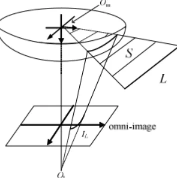
Before introducing the details of the three stages, we give a brief review of the struc- ture of the omni-camera and the associated coordinate systems used in this study. As shown in Fig. 2, the type of omni-camera is catadioptric with the mirror being of a hy- perboloidal shape, which may be described in the camera coordinate system (CCS) as:
2 2
2 2
( )
R Z c 1
a b
− − = − , R= X2+Y2 ,
where a2 + b2 = c2. Specifically, the focal point Om of the mirror is taken to be the origin (0, 0, 0) of the CCS and the camera lens center Oc is located at (0, 0, 2c) in the CCS.
As shown in Fig. 2(b), by triangulation, the camera focal length f may be computed as:
f Dr
= R, (1)
where D, R, and r respectively are the distance from the camera lens center to the mirror base center, the radius of the mirror base in the real-world space, and the radius of the mirror base in the image. Note that the mirror base is of a circular shape. Sub- sequently we will call the left and right cameras as Cameras 1 and 2, and their CCSs as CCS 1 and 2, respectively. A sketch of the proposed method is described in the following.
(a) (b) Fig. 2. Illustration of used omni-directional camera. (a) Camera and hyperboloidal-shaped mirror structure and coordinate systems. (b) Relationship between mirror and image plane.
Algorithm 1. Sketch of the proposed method.
Stage 1. Calibration of camera and mirror parameters.
Step 1. Select a landmark point P in the real-world space.
Step 2. Perform the following steps to calibrate two parameters of Camera 1.
2.1 Measure manually the mirror base radius R1 and the distance D1 between the lens center and the mirror base center in the real-world space.
2.2 Measure manually the location of landmark point P in CCS 1.
2.3 Take an image I1 of P with Camera 1 and extract the image coordinates (u1, v1) of the corresponding pixel p1 from I1.
2.4 Detect the boundary of the mirror base in I1 and compute accordingly the mirror base radius r1.
2.5 Use Eq. (1) to compute the focal length f1 of Camera 1.
2.6 With the location measured in Step 2.2, use a set of analytic formulas (derived later in Sec. 3) to compute the parameter g1 = c1/b1, called mirror distance ratio, where b1 and c1 are the shape parameters of the mirror of Camera 1.
Step 3. Take an image I2 of P with Camera 2 and perform similarly steps to obtain the focal length f2 and the mirror distance ratio g2 of Camera 2.
Stage 2. Computing the optical axis angle by using a line feature on the console table.
Step 4. Place the two camera stands at the left and right sides of the console table with the camera mirror facing forward to the user in front of the table.
Step 5. Take an image of the line feature L of the front boundary of the console table by Camera 1 and extract its pixels.
Step 6. Calculate two parameters (A1, B1) related to the direction of L from the viewpoint of Camera 1 by a Hough transform technique proposed in Sec. 4 with A1 and B1 to be derived in Sec. 4.
Step 7. Take an image of the same line feature L by Camera 2, extract its pixels, and calculate two parameters (A2, B2) related to L from the viewpoint of Camera 2 by the same operations as Steps 5 and 6.
Step 8. Calculate the angle θ between the optical axes of the two cameras in terms of A1, B1, A2, and B2 by an equation derived in Sec. 4 (Eq. (12)).
Stage 3. Acquisition of 3D data of a feature points in the application activity.
Step 9. Measure manually the distance d between the two cameras.
Step 10. Take the images of a feature point P on the user hand by both cameras, and extract the pixels p1 and p2 corresponding to P in the images with coordinates (u1, v1) and (u2, v2), respectively.
Step 11. Calculate the 3D position of P with respect to CCS 1, using the image coordinates (u1, v1) and (u2, v2) as well as the angle θ calculated in Stage 2.
3 Proposed Techniques for Camera Parameter Calibration
The relation between the camera coordinates (X, Y, Z) of a space point P and the im- age coordinates (u, v) of its corresponding projection pixel p in an omni-image I as depicted in Fig. 2(a) may be described [9-12] by:
2 2
2 2
( ) sin 2
tan ( ) cos
b c bc
b c
α β
β
+ −
= − , (2)
2
cos 2
f r
r
= +
β , sin 2 2
f r
f
= +
β , (3)
2 2
tan Z
X Y
α = + , (4)
where r = u2+v2 . The angle α will be called the elevation angle of P. Also, ac- cording to the rotational invariance property of the omni-camera [12], we have the following equalities for describing the azimuth angle θ of p with respect to the u-axis in I and also of P with respect to the X-axis in the CCS:
2 2 2 2
cos X u
X Y u v
θ= =
+ + ,
2 2 2 2
sin Y v
X Y u v
θ= =
+ + . (5)
Traditionally, it is required to calibrate the three camera parameters b, c, and f for gen- eral applications. In this study, alternatively we adopt a more efficient way to compute first the focal length f by Eq. (1), which utilizes the easily-measurable mirror size and the distance between the camera and the mirror base, as described previously. And we then, by using the facts described by Eqs. (2) and (3) above, rewrite Eq. (4) to be
2 2
( 1) sin 2
tan ( 1) cos
g g
g α β
β
+ −
= − (6)
where g is defined as g = c/b. Eq. (6) may be solved to be
2 2 2
1 1 (tan ) (cos ) (sin ) tan cos sin
g α β β
α β β
− ± + −
= − . (7)
If we have a landmark point with known image coordinates (u, v) and known camera coordinates (X, Y, Z), then we can calculate the parameter g by Eqs. (3), (4), and (7).
In real situations, measurement errors and noise might occur, which result in inaccu- racy of the computed value of g. To overcome this difficulty, one can use more than one landmark point to obtain a more accurate result by using non-linear regression or any other curve-fitting technique to get a better value of g fitting to Eq. (6).
4 Proposed Technique to Calculate the Angle between Optical Axes
In this section, we first propose a new technique in Sec. 4.1 to detect a space line in an omni-image and derive the two previously-mentioned parameters A and B to describe the line. The technique is then applied to the line feature of the front console table boundary. Finally, we propose a technique in Sec. 4.2 to calculate the angle between the optical axes of the two omni-cameras, which can be used for 3D feature point data computation.
4.1 Proposed Technique to Detect a Space Line in an Omni-Image
Given a space line L with a point P0 = (X0, Y0, Z0) on the line and with the direction vector vL = (vx, vy, vz), the equation of L may be written according to 3D geometry as
(X, Y, Z) = (X0 + λvx, Y0 + λvy, Z0 + λvz)
where λ is a parameter. As shown in Fig. 3, let S be the space plane going through line L and the mirror base center Om = (0, 0, 0), and let NS = (l, m, n) be the normal vector of S. Then, any point P′ on S with camera coordinates (X, Y, Z) and the mirror base center point Om together form a vector Vm = (X – 0, Y – 0, Z – 0) = (X, Y, Z) which is perpendicular to the normal vector NS = (l, m, n), so that the inner product of Vm and NS becomes zero, leading the following equality:
NS·Vm = lX + mY + nZ = 0 (8)
where “·” means the inner product of two vectors. Combining Eq. (8) with Eqs. (4) and (5) and performing some simplifications, we get
lRcosθ + mRsinθ + nRtanα = 0,
where R = X2+Y2. Dividing both sides of the above equality by R, we get lcosθ + msinθ + ntanα = 0,
which leads to
Acosθ + Bsinθ = −tanα, (9)
with A = l/n and B = m/n. Note that the normal NS = (l, m, n) of plane S now may be expressed alternatively as NS = (A, B, 1).
Fig. 3. Illustration of a space line projected on an omni-image
Eq. (9) describes the projection of a space line onto the omni-image in terms of the azimuth angle θ and the elevation angle α. The equation may be used, as found in this study, to detect the space line projection in an omni-image by a simple Hough trans- form as described next.
Algorithm 2. Computing the parameters for detecting a space line in an omni-image.
Input: The line feature l in an omni-image I (in the form of detected edge points) corresponding to a space line L.
Output: The values of the two parameters A and B in Eq. (9) which describes L.
Step 1. Extract the feature points of the line feature l in the omni-image I by an edge point detection algorithm.
Step 2. Set up a 2D Hough space with two parameters A and B and set all the initial cell values to be zero.
Step 3. Perform the following steps to each pixel of the line feature l with image coordinates (u, v) in I:
3.1 Compute cosβ, sinβ, cosθ, and sinθ by Eq. (5) using u and v.
3.2 Compute tanα by Eq. (6) using the values of cosβ and sinβ, as well as g where the computation of g using landmark points was described at the end of Sec. 3.
3.3 For each cell at parameters (A, B), if cosθ, sinθ, tanα, A, and B satisfy Eq. (9), then increment the cell value by one.
Step 4. Detect the peak cell value in the Hough space and take the corresponding parameters (A, B) as output.
4.2 Calculation of the Angle between the Two Optical Axes
Using Algorithm 2 above we can obtain the parameter pairs (A1, B1) and (A2, B2) to describe a space line L in CCS 1 and CCS 2, respectively. Let the directional vector of the space line L be vL = (vx, vy, vz) again, and let the origin of CCS 1 be denoted as O1.
Also, let S1 be a space plane going through line L and O1. As derived in Sec. 4.1, the normal vector of S1 may be described by n1 = (A1, B1, 1). Since S1 goes through line L, vL and n1 are perpendicular, meaning that
vL·n1 = vxA1 + vyB1 + vz = 0. (10) Furthermore, since the space line L is parallel to the xz-plane of CCS 1 and CCS 2 as assumed (see Sec. 2), we have
vy = 0. (11)
Combining Eqs. (10) and (11), we have vxA1 + vz = 0.
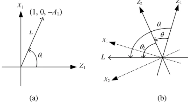
Taking vx be 1 without loss of generality, we get the directional vector of L as vL = (vx, vy, vz) = (1, 0, −A1). Furthermore, as depicted in Fig. 2(a), the optical axis of either camera is parallel to the Z-axis of either CCS. Referring to Fig. 4, we see that the angle between the optical axis of Camera 1 and the space line L can be computed as
1 1
1 2
1
sin ( )
1 A
A θ = − −
+ .
Similarly, the angle between the optical axis of Camera 2 and the space line L can be computed as
1 2
2 2
2
sin ( )
1 A
A θ = − −
+ .
Accordingly, as depicted in Fig. 4, the angle θ between the two optical axes may be computed as
θ = θ1 − θ2 = 1 1
2 1
sin ( )
1 A
A
− −
+ − 1 2
2 2
sin ( )
1 A
A
− −
+ . (12)
The value of θ derived above may be used to compute the 3D data of a feature point, as discussed in the following section.
(a) (b)
Fig. 4. Angles between space line L and optical axes Z1 and Z2. (a) Directional vector of a space line L in CCS 1. (b) Angle between two optical axes.
5 Proposed Technique for Calculating 3D Data of Feature Points
To compute the 3D data of a space point P = (X, Y, Z) from the two omni-images taken by the cameras as described in Stage 3 of Algorithm 1, let the projection of P = (X, Y, Z) in an omni-image taken by Camera 1 be a pixel p1 located at image coordi- nates (u1, v1). From Eqs. (4) and (5), we have
X = Rcosθ1, Y = Rsinθ1, Z = Rtanα1 (13) where cosθ1, sinθ1, and tanα1 can be computed by Eqs. (5) and (6). Eq. (13) can be viewed as one describing a line L1 going through the origin P0 = (0, 0, 0) of CCS 1 with directional vector v1 = (cosθ1, sinθ1, tanα1), and R being a parameter. Note that the coordinates (X, Y, Z) are with respect to CCS 1.
Similarly, let the feature point P be located at (X′, Y′, Z′) in CCS 2, and let its pro- jection in an omni-image taken by Camera 2 be a pixel p2 located at image coordi- nates (u2, v2). Then, similarly to the derivation of Eq. (13) we can obtain:
X′ = Rcosθ2, Y′ = Rsinθ2, Z′ = Rtanα2. (14) With the aid of the angle θ between the two optical axes and the distance d between the two cameras (assumed to be known as mentioned before), we may transform the coordinates (X′, Y′, Z′) in CCS 2 to the coordinates (X, Y, Z) in CCS 1 by the use of a rotation matrix M and a translation vector T described in the following:
T = (d, 0, 0),
cos 0 sin
0 1 0
sin 0 cos
M
θ θ
θ θ
−
⎡ ⎤
⎢ ⎥
=⎢ ⎥
⎢ ⎥
⎣ ⎦
,
or equivalently, we may transform (X′, Y′, Z′) to (X, Y, Z) by the following equation:
2 2 2
' cos 0 sin cos
' 0 1 0 sin 0
' sin 0 cos tan 0
X X R d
Y M Y T R
Z Z R
θ θ θ
θ
θ θ α
−
⎡ ⎤ ⎡ ⎤ ⎡ ⎤ ⎡ ⎤ ⎡ ⎤
⎢ ⎥= ⎢ ⎥+ =⎢ ⎥ ⎢ ⎥ ⎢ ⎥+
⎢ ⎥ ⎢ ⎥ ⎢ ⎥ ⎢ ⎥ ⎢ ⎥
⎢ ⎥ ⎢ ⎥ ⎢ ⎥ ⎢ ⎥ ⎢ ⎥
⎣ ⎦ ⎣ ⎦ ⎣ ⎦ ⎣ ⎦ ⎣ ⎦
which can be viewed as a line L2 going through a point P2 = (d, 0, 0) and with direc- tional vector v2 described as
2 (cos cos 2 sin tan 2, sin 2, sin cos 2 cos tan 2)
v = θ θ − θ α θ θ θ + θ α .
We now have two space lines L1 and L2 going through point P. If everything including the system setup and the camera calibration is accurate without any error, these two lines should intersect precisely at one point P. But unavoidably, errors always exist, and so we estimate in this study the coordinates of point P as those of the mid-point of the shortest line segment between L1 and L2.
6 Experimental Results
A series of experiments have been conducted with a calibration board to test the pre- cision of the proposed system. The board is filled with grid points as shown in Fig. 5.
We used nine of them on the board as landmark points in the experiments.
In an experiment, we put the two camera stands to face forward precisely, with the angle θ between the two camera optical axes being zero. Next, we measured manually the real 3D data of the nine landmark points. Then, we used the proposed method to compute the coordinates of each of the nine points in CCS 1. We define the error ratio of each point Pi at (Xi, Yi, Zi), measured or computed, as
2 2 2
(real Xi computed Xi) (real Yi computed Yi) (real Zi computed Zi) d
− + − + −
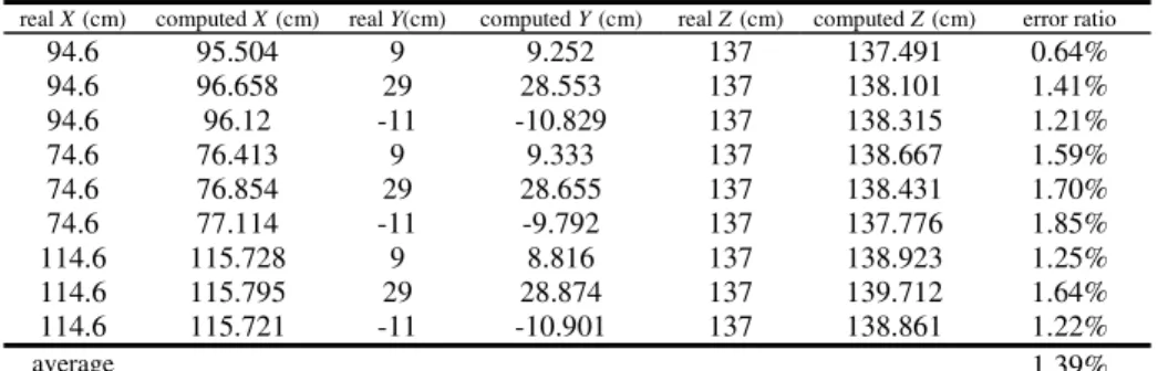
where d is the distance from Pi to the origin of CCS 1. The experimental results are summarized as in Table 1, from which we can see that the computed error ratios are all smaller than 2%, and the average of them is 1.39%.
(a) (b) (c)
Fig. 5. Calibration board used in experiments. (a) Omni-image. (b) Nine calibration points on the board. (c) Calibration points superimposed on the image and shown in red.
Table 1. Error ratios of 3D data computation when two optical axes are mutually parallel
real X(cm) computed X(cm) real Y(cm) computed Y(cm) real Z(cm) computed Z(cm) error ratio
94.6 95.504 9 9.252 137 137.491 0.64%
94.6 96.658 29 28.553 137 138.101 1.41%
94.6 96.12 -11 -10.829 137 138.315 1.21%
74.6 76.413 9 9.333 137 138.667 1.59%
74.6 76.854 29 28.655 137 138.431 1.70%
74.6 77.114 -11 -9.792 137 137.776 1.85%
114.6 115.728 9 8.816 137 138.923 1.25%
114.6 115.795 29 28.874 137 139.712 1.64%
114.6 115.721 -11 -10.901 137 138.861 1.22%
average 1.39%
In another experiment, we simulated the situation that a user sets up the system beside the console table with unintended imprecision: the two camera stands do not face forward precisely. For this, we manually rotated the two camera stands with an unknown angle θ between the two optical axes within a range of about −5° to +5°.
Then, we used the proposed method to automatically detect the value of θ and used it to compute 3D feature point data. Specifically, each image pair taken by the two cam- era stands was processed according to steps in Stage 2 of Algorithm 1 to obtain the angle θ between the two optical axes. An example of experimental results is shown in
Fig. 6, where Fig. 6(a) is an image taken by Camera 1, Fig. 6(b) is the result of edge detection, Fig. 6(c) shows the edges in a region of interest (ROI), Fig. 6(d) is the pa- rameter space of (A, B) produced by the Hough transform, Fig. 6(e) shows the projec- tion of the detected line on the ROI, and Fig. 6(f) shows the projection of the detected line into Fig. 6(a). These results say that the Hough detection result is precise enough for real applications.
Table 2. Average error ratios obtained under imprecise system setup
Computed angle θ between optical
axes
error ratio 1
error ratio 2
error ratio 3
error ratio 4
error ratio 5
error ratio 6
error ratio 7
error ratio 8
error ratio 9
average error ratio -4.21 2.17% 1.83% 2.74% 1.77% 1.87% 1.88% 0.44% 0.89% 1.00% 1.62%
-4.10 0.60% 0.08% 0.53% 0.79% 0.91% 1.58% 0.50% 0.96% 1.07% 0.78%
-3.80 1.63% 1.26% 1.56% 1.26% 1.37% 1.56% 0.63% 0.96% 1.07% 1.25%
-3.16 0.76% 0.19% 1.34% 1.41% 1.44% 1.98% 0.92% 0.42% 0.54% 1.00%
-1.08 1.45% 1.72% 1.43% 2.77% 2.74% 2.73% 1.89% 2.26% 1.28% 2.03%
0.79 2.86% 2.56% 2.88% 2.18% 2.29% 3.31% 2.61% 2.34% 2.65% 2.63%
1.93 4.43% 3.60% 3.91% 3.18% 3.88% 4.33% 3.59% 3.32% 3.63% 3.76%
2.79 2.93% 2.70% 2.37% 2.13% 2.30% 2.68% 2.27% 2.58% 2.84% 2.53%
3.93 2.10% 1.90% 2.15% 1.20% 1.39% 1.88% 2.11% 1.88% 2.15% 1.86%
5.94 2.37% 2.19% 1.83% 1.40% 1.60% 2.05% 2.41% 2.19% 2.45% 2.05%
7.66 0.44% 0.49% 0.49% 1.48% 1.45% 1.70% 0.63% 1.04% 0.71% 0.94%
average 1.86%
(a) (b) (c)
(d) (e) (f) Fig. 6. An experimental result for Stage 2 of Algorithm 1. (a) Omni-image. (b) Edge detec-
tion result. (c) Edges in ROI. (d) Hough space. (e) Projection of peak cell with parameters A = 0.035 and B = 1.395 onto ROI. (f) Projection of detected line onto (a).
After deriving the angle between the optical axes, we measured the distance be- tween two camera stands. Then, we use the nine points on the calibration board as used in Experiment 1 to test the precision of the proposed method in its capability of adaptation to imprecise system setups. The results are summarized in Table 2, from which we see that the average error ratios are still small and the overall average of them is 1.86%.
7 Conclusions
A new two-omni-camera system for 3D vision applications and a method for adapting it to imprecise camera setups have been proposed. First, a novel technique which uses a set of analytic formulas to calibrate omni-directional camera parameters has been proposed. Also, a technique for automatic detection of the angle between the two optical axes of the two cameras resulting from an imprecise camera setup has been proposed. Accordingly, a technique to adapt the system to the imprecise setup has been proposed as well, allowing the system to be able to conduct 3D feature data computation under the imprecise system configuration. Experimental results show that the proposed system and its adaptation capability yield 3D data computation results with average error ratios smaller than 3%, demonstrating the feasibility of the system for general applications.
References
1. Sogo, T., Ishiguro, H., Trivedi, M.M.: N-Ocular Stereo for Real-Time Human Tracking.
In: Benosman, R., Kang, S.B. (eds.) Panoramic Vision, pp. 359–375. Springer, Berlin (2001)
2. Doubek, P., Svoboda, T.: Reliable 3D reconstruction from a few catadioptric images. In:
IEEE Workshop on Omni-directional Vision, pp. 71–78 (2002)
3. Zhu, Z., Rajasekar, K., Riseman, E., Hanson, A.: Panoramic virtual stereo vision of coop- erative mobile robots for localizing 3D moving objects. In: IEEE Workshop on Omnidirec- tional Vision, pp. 29–36 (2000)
4. Jeng, S.W., Tsai, W.H.: Analytic image unwarping by a systematic calibration method for omni-directional cameras with hyperbolic-shaped mirrors. Image and Vision Comput- ing 26(5), 690–701 (2008)
5. Wu, C.J., Tsai, W.H.: Unwarping of images taken by misaligned omni-cameras without camera calibration by curved quadrilateral morphing using quadratic pattern classifiers.
Optical Engineering 48(8), Article no. 087003 1–11 (2009)
6. Fabrizio, J., Tarel, J.-P., Benosman, R.: Calibration of panoramic catadioptric sensors made easier. In: IEEE Workshop on Omni-directional Vision, pp. 45–52 (2002)
7. Mei, C., Rives, P.: Single View Point Omnidirectional Camera Calibration from Planar Grids. In: IEEE International Conference on Robotics and Automation, pp. 3945–3950 (2007)
8. Wu, C.J., Tsai, W.H.: An omni-vision based localization method for automatic helicopter landing assistance on standard helipads. In: International Conference on Computer and Automation Engineering, Singapore, pp. 327–332 (2010)
9. Gaspar, J., Winters, N., Santos-Victor, J.: Vision-based navigation and environmental rep- resentations with an omni-camera. IEEE Transactions on Robotics and Automation 16(6), 890–898 (2000)
10. Mashita, T., Iwai, Y., Yachida, M.: Calibration method for misaligned catadioptric camera.
IEICE Transactions on Information & Systems E89-D(7), 1984–1993 (2006)
11. Ukida, H., Yamato, N., Tanimoto, Y., Sano, T., Yamamoto, H.: Omni-directional 3D Measurement by Hyperbolic Mirror Cameras and Pattern Projection. In: IEEE Conference on Instrumentation and Measurement Technology, pp. 365–370 (2008)
12. Jeng, S.W., Tsai, W.H.: Using pano-mapping tables to unwarping of omni-images into panoramic and perspective-view Images. IET Image Processing 1(2), 149–155 (2007)