A Two-omni-camera Stereo Vision System with an Automatic Adaptation Capability to Any
System Setup for 3D Vision Applications
Shen-En Shih and Wen-Hsiang Tsai, Senior Member, IEEE
Abstract—A stereo vision system using two omni-cameras for 3D vision applications is proposed, which has an automatic adaptation capability to any system setup before 3D data computation is conducted. The adaptation, which yields the two omni-cameras’ orientations and distance, is accomplished by detecting and analyzing the horizontal lines appearing in the omni-images acquired with the cameras and a person standing in front of the cameras. Properties of line features in environments are utilized for detecting more precisely the horizontal lines which appear as conic sections in omni-images. The detection work is accomplished by the use of carefully chosen parameters and a refined Hough transform technique. The detected horizontal lines are utilized to compute the cameras’ orientations and distance from which the 3D data of space points are derived analytically.
Compared with a traditional system using a pair of projective cameras with nonadjustable camera orientations and distance, the proposed system has the advantages of offering more flexibility in camera setups, better usability in wide areas, higher precision in computed 3D data, and more convenience for non-technical users.
Good experimental results show the feasibility of the proposed system.
Index Terms—system setup, automatic adaptation, 3D vision applications, omni-camera, omni-image, stereo vision.
I. INTRODUCTION
ith the advance of technologies, various types of vision systems have been designed for many applications, like virtual and augmented reality, video surveillance, environment modeling, TV games, etc. Among these applications, human-machine interaction is a critical area [1]-[4]. For example, Microsoft Kinect [5] is a controller-free gaming system in the home entertainment field, which uses several sensors to interact with players. Most of these human-machine interaction applications require acquisitions of the 3D data of human bodies, meaning in turn the need of precise system calibration and setup works to yield accurate 3D data computation results in the application environment.
However, from a consumer’s viewpoint, it is unreasonable to ask a user to set up a vision system very accurately, requiring, e.g., the system cameras to be affixed at accurate locations in precise orientations. Contrarily, it is usually desired to allow a user to choose freely where to set up the system components.
Additionally, many interactive systems used for the previously-mentioned applications are composed of traditional projective cameras which collect less visual information than systems using omni-directional cameras (omni-cameras). To overcome these difficulties, a 3D vision system which consists of two omni-cameras with a capability of automatic adaptation to any camera setup is proposed. While establishing the system, the user is allowed to place the two cameras freely in any orientations with any displacement.
Human-machine interaction has been intensively studied for many years. Laakso and Laakso [6] proposed a multiplayer game system using a top-view camera, which maps player avatar movements to physical ones, and uses hand gestures to trigger actions. In [7], a special human-machine interface is proposed by Magee et al., which uses the symmetry between left and right human eyes to control computer applications.
Zabulis et al. [8] proposed a vision system composed of eight cameras mounted at room corners and two cameras mounted on the ceiling to localize multiple persons for wide-area exercise and entertainment applications. Starck et al. [9] proposed an advanced 3-D production studio with multiple cameras. The design considerations are first identified in that study, and some evaluation methods are proposed to provide an insight into different design decisions.
Geometric features, like points, lines, spheres, etc., in environments encode important information for on-line calibrations and adaptations [10][11]. Several methods have been proposed to detect such features in environments. Ying [12][13] proposed several methods to detect geometric features when calibrating catadioptric cameras, which use the Hough transform to find the camera parameters by fitting detected line features into conic sections. Duan et al. [14] proposed a method to calibrate the effective focal length of the central catadioptric camera using a single space line under the condition that other parameters have been calibrated previously. Von Gioi et al.
[15] proposed a method to detect line segments in perspective images, which gives accurate results with a controlled number
W
This work was supported in part by a grant from the Ministry of Economic Affairs, Republic of China under Project No. MOEA 98-EC-17-A-02-S1-032 in the Technology Development Program for Academia.
S. E. Shih is with the Institute of Computer Science and Engineering, National Chiao Tung University, Hsinchu, Taiwan 30010. E-mail:
W. H. Tsai is with the Department of Computer Science, National Chiao Tung University, Hsinchu, Taiwan 30010. He is also with the Department of Information Communication, Asia University, Taichung, Taiwan 41354.
E-mail: [email protected].
of false detections and requires no parameter tuning. Wu and Tsai [16] proposed a method to detect lines directly in an omni-image using a Hough transform process without unwarping the omni-image. Maybank et al. [17] proposed a method based on the Fisher-Rao metric to detect lines in paracatdioptric images, which has the advantage that it does not produce multiple detections of a single space line. Yamazawa et al. [18] proposed a method to reconstruct 3D line segments in images taken with three omni-cameras in known poses based on trinocular vision by the use of the Gaussian sphere and a cubic Hough space [19]. Li et al. [20] proposed a vanishing point detection method based on cascaded 1-D Hough transforms, which requires only a small amount of computation time without losing accuracy.
In this study, we propose a new 3D vision system using two omni-cameras, which has a capability of automatic adaptation to any system setup for convenient in-field uses. Specifically, the proposed vision system, as shown in Fig. 1, consists of two omni-cameras facing the user’s activity area. Each camera is affixed firmly to the top of a rod, forming an omni-camera stand, with the camera’s optical axis adjusted to be horizontal (i.e., parallel to the ground). The cameras are allowed to be placed freely in the environment at any location in any orientation, resulting in an arbitrary system setup. Then, by the use of space line features in environments, the proposed vision system can adapt automatically to the arbitrarily-established system configuration by just asking the user to stand still for a little moment in the middle region of the activity area in front of the two cameras. After this adaptation operation, 3D data can be computed precisely as will be shown by experimental results in this paper.
As an illustration of the proposed system, Fig. 1(c) shows the case of a user using a cot-covered fingertip as a 3D cursor point, which is useful for 3D space exploration in video games, virtual/augmented reality, 3D graphic designs, and so on. The fingertip is detected and marked as red in that figure, whose 3D location can be computed by triangulation.
In contrast with a conventional vision system with two cameras whose configuration is fixed, the proposed system has several advantages. First, the system can be established freely, making it suitable for wide-ranging applications. This is a highly desired property especially for consumer electronics applications such as home entertainment or in-house surveillance, since the user can place the system components flexibly without the need to adjust the positions of the existing furniture in the application environment. Second, since the proposed vision system uses omni-cameras, the viewing angle of the system is very wide. This can be seen as an improvement over commercial products like Microsoft Kinect since the player can now move more freely at a close distance to the sensors. This advantage is very useful for people who only have small spaces for entertainments. Also, the two cameras in the proposed system are totally separated from each other at a larger distance, resulting in the additional merit of yielding better triangulation precision and 3D computation results due to the resulting longer baseline between the two cameras.
X1
Y1
Z1
X2
Y2
Z2
(a)
(b) (c) Fig. 1. Configuration and an illustration of the usage of proposed system. (a)
An illustration. (b) Real system used in this study. (c) An omni-image of a user wearing a finger cot (marked as red).
In the remainder of this paper, an overview of the proposed system is described in Section II, and the details of the proposed techniques for use in the system are presented in Sections III through VI. Experimental results are included in Section VII, followed by conclusions in Section VIII.
II. OVERVIEW OF PROPOSED SYSTEM
The use of the proposed system for 3D vision applications includes three stages: (1) in-factory calibration; (2) in-field system adaptation; and (3) 3D data computation. The goal of the first stage is to calibrate the camera parameters efficiently in the factory environment. For this, a technique using landmarks and certain conveniently-measurable system features is proposed. In the second stage, an in-field adaptation process is performed, which uses line features in environments to automatically compute the orientations of the cameras and the distance between them (i.e., the baseline of the system). In this stage, a user with a known height is asked to stand in the middle region in front of the two cameras to complete the adaptation.
Subsequently, the 3D data of any feature point (like the finger tip shown in Fig. 1(c)) can be computed in the third stage.
A sketch of the three operation stages of the proposed system is described in the following. To simplify the expressions, we will call the left and right cameras as Cameras 1 and 2, and their camera coordinate systems as CCSs 1 and 2, respectively.
Algorithm 1. Sketch of the proposed system’s operation.
Stage 1. Calibration of omni-cameras.
Step 1. Set up a landmark and select at least two feature points Pi on it, called landmark points.
Step 2. Perform the following steps to calibrate Camera 1.
2.1. Measure manually the radius of the mirror base of the camera as well as the distance between the camera and the mirror, as stated in Section VII-A.
2.2. Take an omni-image I1 of landmark points Pi with Camera 1 and extract the image coordinates of those pixels pi which correspond to Pi.
2.3. Detect the circular boundary of the mirror base in I1,
compute the center of the boundary as the camera center, and derive accordingly the focal length f1 of the camera, as described in Section VII-A.
2.4. Calculate the eccentricity of the hyperboloidal mirror shape using the coordinates of pi and those of Pi, as stated in Section VII-A.
Step 3. Take an image I2 of landmark points Pi with Camera 2 and perform operations similar to those of the last step to calibrate the camera to obtain its focal length f2 and eccentricity .
Stage 2. Adaptation to the system setup.
Step 4. Place the two camera stands at proper locations with appropriate orientations to meet the requirement of the application activity.
Step 5. Perform the following steps to calculate the included angle between the two optical axes of the cameras as shown in Fig. 1(a).
5.1. Capture two omni-images I1 and I2 of the application activity environment with Cameras 1 and 2, respectively.
5.2. Detect space line features Li in omni-image I1 using the Hough transform technique as well as the parameters f1 and 1, as described in Section IV.
5.3. Detect space line features Ri in omni-image I2
similarly with the use of the parameters f2 and 2. 5.4. Calculate angle using the detected line features Li
and Ri in a way as proposed in Section V.
Step 6. Perform the following steps to calculate the orientations of the two cameras and the baseline between them.
6.1. Ask a user of the system to stand in the middle region in front of the two omni-cameras and take two images of the user using the cameras.
6.2. Extract from the acquired images a pre-selected feature point on the user’s body, and compute the respective orientations and of the two cameras using the angle , as described in Section VI-A.
6.3. Detect the user’s head and foot in the images, compute the in-between distance up to a scale, and use the distance as well as the corresponding known height of the user to calculate the baseline D between the cameras, as described in Section VI-C.
Stage 3. Acquisition of 3D data of space points.
Step 7. Take two omni-images of a selected space feature point P (e.g., a fingertip, a handed light point, a body spot, etc.) with both cameras, and extract the corresponding pixels p1 and p2 in the taken images.
Step 8. Calculate as output the 3D position of P in terms of the coordinates of p1 and p2, the focal lengths f1 and f2, the eccentricities 1 and 2, the orientations 1
and 2, and the baseline D, using a triangulation based method described in Section VI-B.
Via the above algorithm, the meaning of system adaptation, which is the main theme of this study, can be made clearer now:
only with the input of the knowledge of the user’s height (see Step 6.3), the proposed system can infer the required values of the cameras’ orientations and 2 and baseline D for use in computing the 3D data of space points. This is not the case when using a conventional stereo vision system with two cameras in which the configuration of the cameras are fixed
with their orientations and baseline unchangeable. This merit of the proposed system makes it easy to conduct system setup in any room space by any people for more types of applications, as mentioned previously.
III. STRUCTURE OF OMNI-CAMERAS
The structure of omni-cameras used in this study and the associated coordinate systems are defined as shown in Fig. 2.
An omni-camera is composed of a perspective camera and a hyperboloidal-shaped mirror. The geometry of the mirror shape can be described in the camera coordinate system (CCS) as:
2 2 2
2 2
( )
Z c X Y 1
a b
, a2 + b2 = c2, Z < c.
The relation between the camera coordinates (X, Y, Z) of a space point P and the image coordinates (u, v) of its corresponding projection pixel p may be described [22] as:
2
2 2 2
( 1)sin 2
tan ( 1)cos
Z X Y
; (1)
2 2
cos r
r f
;
2 2
sin f
r f
; r = u2v2, (2) where is the eccentricity of the mirror shape with its value equal to c/a, and and are the elevation and azimuth angles of P, respectively. The azimuth angle can be expressed in terms of the image and camera coordinates as
cos 2X 2 2u 2; sin 2Y 2 2v 2.
X Y u v X Y u v
IV. SPACE LINE DETECTION IN OMNI-IMAGES
We now describe the proposed method to detect horizontal space lines in omni-images. Several ideas adopted to design the method are emphasized first. First, it is desired to eliminate initially as many non-horizontal space lines in each acquired image as possible since only horizontal space lines are used to find the included angle as described later in Section V. Second, it is hoped that the method can deal with large amounts of noise so that it can be used in an automatic process. Third, it is desired to utilize certain properties in man-made environments to improve the detection result, including the two properties that space lines are mostly horizontal or vertical, and that space line edges are usually not close to one another.
Fig. 2. Camera and hyperboloidal-shaped mirror structure.
This uadratic fo
which goes th
(4)
here “” denotes Combining (4
mRsin + nRtan = 0, (5) here R =
section is organized as follows. First, a q
rmula describing the projection of a space line in an omni-image is derived in Section IV-A. Next, a refined Hough transform technique for detecting space lines is proposed in Section IV-B, which uses a novel adaptive thresholding scheme to produce robust detection results. Also, the projection of a vertical space line is derived and analyzed in Section IV-C. A peak cell extraction technique proposed for use in the refined Hough process is described at last in Section IV-D.
A. Projection of a Space Line in an Omni-Image Given a space line L, we can construct a plane S
rough L and the origin Om of a CCS as shown in Fig. 3. Let NS
= (l, m, n) denote the normal vector of S. Then, any point P = (X, Y, Z) on L satisfies the following plane equation:
NS·P = lX + mY + nZ = 0.
w the inner-product operator. )
with (1) and (3), we get lRcos +
w X2Y2. Dividing (5) by R l2m2n2 leads to
2 2 2 2 2 2 2 2 2
cos sin
l m tan
n 0
l m n l m n l m n
,
which can be transformed into the following form
Acos 1A2B2sinBtan0
ith the two parameters A and B defined as w
2 2 2
A l
l m n l2m2n2
Accordingly, the normal vector NS of plane S, originally being B n
(l, m, n), can now be expressed alternatively as
NS( , 1A A2B2, )B
is assumed that m 0 in (6) and (8) above. In case that m <
It 0,
we may consider NS = (l, m, n) instead, which also represents the same space plane S. Also, it can be seen from (7) that, parameters A and B satisfy the constraint A2 + B2 ≤ 1, implying that the Hough space is of a circle shape.
Fig. 3. Illustration of a space line L projected on an omni-image as IL.
The parameters A and B are used in the Hough transform to detect space lines in omni-images. These two parameters are skillfully defined in (7), leading to several advantages. First, removals of vertical space lines can be easily achieved by ignoring periphery regions as described later in Section IV-C.
Next, since the possible values of A and B range from 1 to 1, the size of the Hough space is fixed within this range. This is a necessary property in order to use the Hough transform technique, and is an improvement on a previous work [16].
Also, the parameters A and B are used directly to describe the directional vector of the space line L as will be shown later in
(1 s to
yi
4). Hence, one may divide the Hough space into more cell eld a better precision.
Combining (6) with (1) through (3), we can derive a conic section equation to describe the projection of a space line L onto an omni-image as follows:
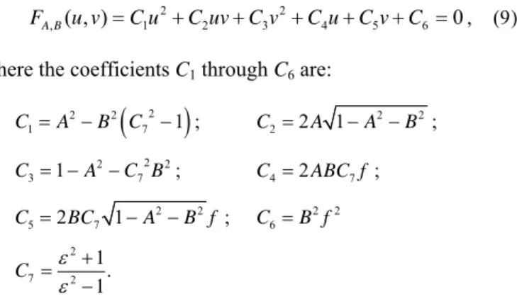
FA B, ( , )u v C u1 2C uv C v2 3 2C u4 C v5 C6 0 where the coefficients C1 through C6 are:
2
2 2
1 7 1
C A B C ; C22A 1A2B2;
2 2 2
3 1 7
C A C B ; C42ABC f7 ;
2 2
5 2 7 1
C BC A B f ; C6B f2 2
2
7 2
1. C 1
The quadratic formula (9) will be called the target equa ntio in the Hough transform subsequently, since the goal of the
cribed by it in an omni-image.
B. Hough Space Generation with Adaptive Thresholding We define the Hough space to be two-dim
eters A and B descri ousl efine the cell support for a cell at (A, B) i
ulation of
e value of tha scribed by the
two parameters (A, B). Two properties of cell supports are
ore, it is desired that the shape of the cell support is of a certain fixed width and not too “thin,” so that tion er
detection process is to find curves des
ensional with the
param bed previ y. Furthermore, we
d n the Hough space as
the set of those pixels which contribute to the accum th t cell. Let L denote a space line de
desirable: (1) the pixels of the projection IL of L onto the omni-image are all included in the cell support for the cell (A, B); and (2) the pixels not on IL are not included in this cell support. Furtherm
(edge) pixels originally belonging to IL but with small detec rors can still contribute to the cell value. In short, a cell support is desired to be a space line projection with a certain width everywhere along the line, which is called an equal-width projection curve hereafter. In this section, we first show that commonly-used curve detection methods do not generate desired equal-width projection curves as cell supports as shown in Figs. 4(a) and 4(b), so we propose in this study an adaptive method to solve this problem to yield better results like the one shown in Fig. 4(c).
(a) (b) (c) Fig. 4. Shapes of cell supports of four chosen Hough cells yielded by three
methods. (a) Using traditional accumulation method. (b) Using a threshold = 3000. (c) Using the proposed technique.
A commonly-used method for curve detection to calculate the cell support is as follows [30][31][32]: for each pixel at coordinates (u, v), find all the Hough cells with their parameter values (A, B) satisfying the target equation (9), and increment the value of each cell so found by one. Some cell supports calculated by this m thod are shown in g. 4(a), showing that the cell supports for some cel re not with equal dths.
Another straightforward m o calculate the l support
i ch
( s
w ation
e Fi
ls a ethod t
wi cel s as follows [16][33]: define a threshold first, and for ea edge) pixel with coordinates (u, v), find all the Hough cell
ith their parameters (A, B) satisfying the equ
2 2
, ( , ) 1 2 3 4 5 6
FA B u v C u C uvC v C uC vC and increment the value of each cell so found by one. However, as shown in Fig. 4(b), it is impossible to find a good threshold which makes all the projection curves to be of equal widths. To solve this problem, it is necessary to develop a new method to adaptively determine the threshold value for each different ce
ingly. For this aim, the method we propose makes a novel use of total
erivatives to estimate the function values of F on the bo and sets the threshold value in (10) accordingly. More
ll support and each different pixel.
Conceptually, to draw an equal-width curve of F = 0, we have to compute the function values of F on the projection curve boundary, and define the threshold accord
d undary,
specifically, is set in the proposed method to be
, ,
( , ) ( 1, 1)
( , , , ) max A B A B
u v
F F
A B u v u v
u v
for different Hough cells with parameters (A, B) and different pi
Additional Constraint on Vertical Space Lines
In man-made environments, most lines are either parallel to
nes from the de
e vertically placed on the floor, with the Y-axis of the camera coordinate As a result, th
, results in the equality A2
and horizontal
hords in omn of horizontal
n environment mostly are not so close mutually, meaning that es usually are separated for a certain di
xels at coordinates (u, v). Accordingly, as shown in Fig. 4(c), the drawn curves are now with uniform widths.
As a summary, the Hough space can be generated using (10) with threshold calculated by (11). With this improvement, the cell supports become equal-width projection curves, making the Hough transform process more robust to yield a precise peak value which represents a detected space line.
C.
the floor (which is called horizontal space lines hereafter) or perpendicular to the floor (which is called horizontal space lines). If we can eliminate vertical space li
tection results, the rest of them are much more likely to be horizontal ones which are desired as stated later in Section V.
In this section, a constraint on the vertical space line is derived for the purpose of removing such lines.
As mentioned earlier, the omni-camera stands ar system being a vertical line as depicted in Fig. 1(a).
e directional vector vL of a vertical space line L is just (0, 1, 0).
Let S be the space plane going through L and the origin Om
which is at camera coordinates (0, 0, 0). Also, let NS = (l, m, n) be the normal vector of plane S. By definition, normal vector NS
is perpendicular to vL, leading to the constraint:
NSvL = (l, m, n)(0, 1, 0) = m = 0.
This constraint, when combined with (7)
+ B2 = 1, which shows subtly that the Hough cells of vertical space lines are located in the periphery region of the circular Hough space (as mentioned earlier in Section IV-A). As a result, vertical space lines can be easily removed by just ignoring the periphery region of the Hough space. In the proposed method, this is achieved automatically by applying a filter on the Hough space as described next in Section IV-D.
Note that, in general, vertical and horizontal space lines do not correspond to curve segments with vertical
c i-images. In fact, the projections
space lines may be with any direction as shown in Fig. 11(f).
Also, the removal of a vertical space line will sometimes also eliminate a few horizontal space lines lying on the plane which goes through the vertical space line and the origin of the camera coordinate system. However, as shown in Figs. 7(a), 7(b), 11(e), and 11(f), many horizontal space lines can still be extracted.
D. Peak Cell Extraction
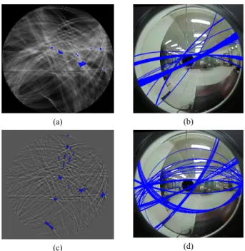
After the Hough space is generated, the last thing to do is to extract cells with peak values, called peak cells, which represent the detected space lines. The simplest way to accomplish this is to find the cells with large values. However, if we do so to get peak cells like those shown in Fig. 5(a), we might get a bad detection result like that shown in Fig. 5(b) with many of the detected space lines being too close to one another, from which less useful space lines may be extracted.
To solve this problem, we notice that the line edges in a two detected horizontal lin
stance. This in turn means that extracted peak cells should not be too close to one another. To find the peak cells which are not too close to each other, a filter is applied on the Hough space:
1 1 1 1 1
1 1 1 1 1
1 1 1 24 1 1
25 1 1 1 1 1
1 1 1 1 1
. (12)
Th
Section IV-C: the removal of the periphery region is equivalent to the removal of vertical space lines. Thus, expectedly we can
et more horizontal lines as desired. To
proposed a new method to detect horizontal space lines in omni-images, with several novel techniques also proposed in Sections IV-A through IV-D to improve the detection result.
(u, v, A, B) satisfies (10) in which the threshold value is valu
described by (12) to Hough space H, Bi) as output.
en, we extract peak cells by choosing the cells with large values in the filtered Hough space to yield a better detection result, as shown by Figs. 5(c) and 5(d).
By the way, it is noted that when applying the filter to the Hough space, one of the side effects is the removal of the periphery region. This is a desired property mentioned in
g sum up, we have
The proposed method for horizontal space line detection is summarized as an algorithm in the following.
Algorithm 2. Detection of horizontal space lines in the form of conic sections in an omni-image.
Input: an omni-image I.
Output: 2-tuple values (Ai, Bi) as defined in (7) which describe detected horizontal space lines in I.
Step 1. Extract the edge points in I by an edge detection algorithm [25].
Step 2. Set up a 2D Hough space H with two parameters A and B, and set all the initial cell values to be zeros.
Step 3. For each detected edge point at coordinates (u, v) and each cell C with parameters (A, B), if
adaptively calculated by (11), then increment the e of C by one.
Step 4. Apply the filter
choose those cells with maximum values, and take their corresponding parameters (Ai,
(a) (b)
(c) (d)
Fig. 5. Comparison of traditional peak cell extraction method and proposed one. (a) Hough space. (b) 50 detected e lines using traditional method. (c) Post-processed Hough space. (d) 50 detected space lines using proposed method.
V. CALCULATION OF INCLUDED ANGLE BETWEEN TWO
CAMERAS’OPTICAL AXES USING DETECTED LINES
In the proposed vision system, the omni-cameras are mounted on two vertical stands with the optical axes being parallel to the floor plane as mentioned previously, but the cameras’ optical axes are allowed to be non-parallel, making an included angle as depicted in Fig. 1(a). To accomplish the 3D ation work under an arbitrary system setup, the l ust be calculated first. A m o calculate
t e
l o
c to
c ng multiple automatically extracted horizontal space lines. To achieve this, a novel method is
d
spac
data comput
included ang e m ethod t
he angle using a single manually chosen horizontal spac ine is proposed first in Section V-A. However, in order t onduct the adaptation process automatically, we have alculate the angle usi
proposed next in Section V-B, which utilizes all the detecte space lines from the two omni-images taken with the cameras.
The proposed method has several advantages. First, only the directional information of the space line, which is a robust feature against noise, is used. Next, no line correspondence between the two omni-images need be derived; that is, it is unnecessary to decide which line in the left omni-image corresponds to which one in the right omni-image. This makes the proposed method fast, reliable, and suitable for a wide-baseline stereo system like the one proposed in this study.
Also, the proposed method makes use of a good property of the man-made environment — many line edges in such environments are parallel to one another, leading to an improvement on the robustness and correctness of the computation result.
A. Calculating Angle Using a Single Horizontal Space Line In this section, a method to calculate the angle between the two cameras’ optical axes is proposed, using a single horizontal space line L in the environment. Let (A1, B1) be the parameters corresponding to line L in an omni-image taken with Camera 1, vL = (vx, vy, vz) be the directional vector of L in CCS 1, and S1 be the space plane going through line L and the origin of CCS 1.
The normal vector of S1 can be derived, according to (8), to be
2 2
1 ( , 11 1 1 , 1)
n A A B B .
Since S1 goes through line L, we get to know that vL and n1 are perpendicular, resulting in the following equality:
vL·n1 = v Ax 1vy 1A12B12v Bz 10. (13) Furthermore, since L, being horizontal, is parallel to the XZ-plane as shown in Fig. 1(a), we get another constraint vy = 0.
This constraint can be combined with (13) to get
vL = (vx, vy, vz) = (B1, 0, A1). (14) Next, by referring to Fig. 6(a), it can be seen that the angle 1
between the X-axis of CCS 1 and space line L is
1 = tan1(A1/B1).
B1,0,A1
(a) (b)
Fig. 6. Illustration o
2 2 ng to the
orizontal space line
derivations described above, the angle 2 between the X-axis of CCS 2 and line L can be derived to be
2 = tan1(A2/B2).
As depicted in Fig. 6(b) where L1 and L2 specify identically the single horizontal space line L, the angle between the two cameras’ optical axes can now be computed easily to be
= 1 2 = tan 1(A1/B1) tan1(A2/B2). (15) B.
an be detected from an omni-image using Algorithm 2 as described in Section IV. Let L1 be a space lin
he space lines L1 and L2
are an identical horizontal space line i the environment.
However, the line roblem of deciding
s and ewing fi
nvironme
ca
of th
value for an
t wij. After such a w
f the angles 1, 2 and . (a) The definition of 1. (b) Relation between 1, 2 and .
Similarly, let (A , B ) be the parameters correspondi
h L in Camera 2. By following the same
Calculating Angle Reliably Using Several Detected Lines Horizontal space lines c
e so detected from the left omni-image with parameters (A1, B1), and let L2 be another detected similarly from the right omni-image with parameters (A2, B2). As stated previously, the angle can be calculated using (15) if t
L n correspondence p
whether L1 and L2 are identical or not is difficult for several reasons, especially for a wide-baseline stereo system like the one proposed in this study. First, the respective viewpoint vi elds of the two cameras differ largely. Thus, e nt features, like lighting and color, involved in the image-taking conditions at the two far-separated cameras might vary largely as well. Also, the extrinsic parameters of the two meras are unknown; therefore, the involved geometric relationship is not available for use to determine the line correspondences. To get rid of these difficulties, we propose a novel statistics-based method to reliably find the angle without the need to find such line correspondences.
More specifically, the proposed method makes use of two important properties. First, it is noticed that the correct value
e angle can still be calculated using (15) even when the two space lines L1 and L2 are not an identical one, but are parallel to each other. This can be seen from the fact that the angles 1 and
2 remain the same if L1 and L2 are parallel so that the computed angle is still correct, as desired. Second, it can be seen that in man-made environments, many of the line edges are parallel to one another in order to make the environment neat and orderly.
For example, tables, shelves, and lights are always placed to be parallel to walls and to one another. Combining these two
properties, we can conclude that any two detected space lines L1 and L2 are very likely to be parallel to each other. Based on this observation, we assume every possible line pair L1 and L2
to be parallel, and compute accordingly a candidate
gle , where L1 is one of the space lines detected from the left omni-image, and L2 is another detected from the right omni-image. Then, we infer a correct value for angle from the set of all the computed candidate values via a statistical approach based on the concept of “voting.”
In more detail, the proposed method is designed to include three main steps. First, we extract space lines from the left omni-image as described in Algorithm 2, and denote the line parameters (A, B) of them as li. Similarly, we detect space lines from the right omni-image with their parameters denoted as rj. In addition, we define two weights w(li) and w(rj) for li and rj, respectively, to be the cell values in the post-processed Hough space derived in Step 4 of Algorithm 2, which represent the trust measures of the detected space lines. Then, from each possible pair (li, rj), we calculate a value ij for angle using (15), as well as a third weight wij defined as w(li)w(rj). The value wij may be regarded as the trust measure of the calculated angle ij. Finally, we set up a set of bins, each for a distinct value of , and for each computed value ij, we increase the value of the corresponding bin by the weigh
eight accumulation work is completed, the bin with the largest value is found out and the corresponding angle ij is taken as the desired value for angle .
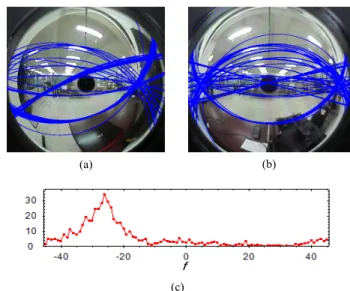
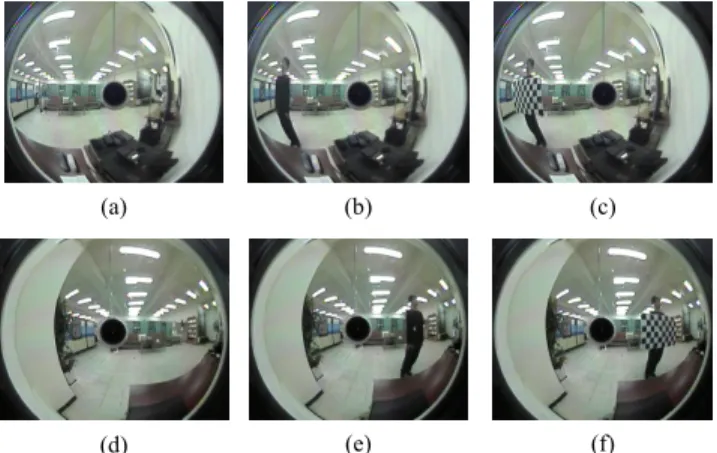
An experimental result so obtained is shown in Fig. 7. In Figs.
7(a) and 7(b), fifty space lines with parameters li and rj were detected using Algorithm 2 from the left and right omni-images, respectively. For each possible pair (li, rj) where 1≤i, j≤50, the corresponding angle ij and weight wij were calculated and accumulated in bins as described previously. The accumulation result is shown in Fig. 7(c) with the maximum occurring at =
23°, which is taken finally as the derived value of angle .
(a) (b)
(c)
Fig. 7. Experimental result of proposed adaptation method for detecting included angle . (a) and (b) Left/right omni-images, with the detected space lines superimposed on it. (c) Accumulation result for with maximum occurring at = 23°.
VI. PROPOSED TECHNIQUE FOR BASELINE DERIVATION AND
ANALYTIC COMPUTATION OF 3DDATA
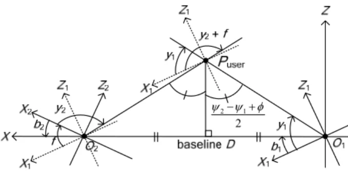
The world coordinate system X-Y-Z is defined as depicted in Fig. 8. The X-axis goes through the two camera centers O1 and O2; the Y-axis is taken to be parallel to the Y-axes of both CCSs;
the Z-axis is defined to be perpendicular to the XY-plane; and the origin is defined to be the origin O1 of CCS 1. It is noted here that, since the two omni-cameras are affixed firmly on the omni-camera stands and adjusted to be of an ntical height as described in Section I, the axes X, Z, X1, Z1, X2, and Z2 are all on the same plane as illustrated in Fig. 8.
Since the two omni-cameras are allowed to be placed arbitrarily at any location with any orientation, it is necessary to find the baseline D and the orientation angles 1 and (as defined in Fig. 8) in advance to calculate the 3D data of space points. A novel method to cal ate the orientation angles is
p re
d as
d
h ine the baseline D is proposed in
as proposed i
1 2
ide
2
cul
roposed first in Section VI-A. After the orientations a erived, the 3D data can be determined up to a scale iscussed in Section VI-B. Then, a method using the known eight of the user to determ
Section VI-C. After the baseline D is derived, the absolute 3D data of space feature points can be derived by a similar method n Section VI-B. It is emphasized that all computations involved in these steps are done analytically, i.e., by the use of formulas without resorting to iterative algorithms.
A. Finding Two Cameras’ Orientations
Let the camera coordinates of CCS 1 be denoted as (X1, Y1, Z1), and those of CCS 2 as (X2, Y2, Z2), as shown in Fig. 8. As mentioned previously, the two CCSs X1-Y1-Z1 and X2-Y2-Z2 are allowed to be oriented arbitrarily (with Y and Y parallel to each other), and the only knowledge acquired by the proposed system is the angle between the two optical axes Z1 and Z2, which is derived using the detected space lines, as described previously in Section V.
To derive the angles 1 and 2, the user is asked to stand in the middle region in front of the two omni-cameras so that a feature point Puser on the user’s body may be utilized to draw a mid-perpendicular plane of the line segment O1O2 as shown in Fig. 8. Let (X1, Y1, Z1) be the coordinates of Puser in CCS 1, and (u1, v1) be the corresponding pixel’s image coordinates in the left omni-image. From (1) and (3), we have the equality:
X1 Y1 Z1
T X12Y12
cos1 sin1 tan1
T, where cos1, sin1, and tan1 are computed from (u1, v1)ows that the according to (1) and (3). This equality sh
directional vector between O1 and Puser is (cos1, sin1, tan1) in CCS 1. An angle 1 is defined on the XZ-plane as illustrated in Fig. 8, which can be expressed as 1 = tan1(tan1/cos1).
Similarly, the angle 2 defined on the XZ-plane can be derived to be tan1(tan2/cos2). Accordingly, we can derive 1 to be
2 1 1 2
1 1
2 2 2 2
,
2 1
2
Fig. 8. A top-view of the coordinate systems. The baseline D, orientation angles 1 and 2, and a point Puser on the user’s body are also drawn.
and 2 is just 2 = 1 . This completes the derivations of the orientation angles 1 and 2 of the two cameras.
B. Calculating 3D Data of Space Feature Points
Let P be a space feature point with coordinates (X, Y, Z) in CCS 1, and let the projection of P onto the omni-image taken
y Camera 1 be the pixel p1 located at image coordinate From (1) and (3) with R1 =
b s (u1, v1).
2 2
1 1
X Y , we have
X1 Y1 Z1
TR1
cos1 sin1 tan1
T (16) where cos1, sin1, and tan1 are computed from (u1, v1) by (1) and (3). Equation (16) describes a light ray L1 going through the origin O1 with directional vector d1′ = [cos1 sin1 tan1]T in CCS 1. To transform the vector into the coordinate system X-Y-Z, we have to rotate d1′ along the Y-axis through the angle1 as illustrated in Fig. 8. As a result, the transformed light ray L1 goes through (0, 0, 0) with its directional vector d1 being
d1 =
1 1 1
cos 0 sin cos
0 1 0 sin 1
1 1 1
sin 0 cos tan
.
Similarly, let the space feature point P be located at ( (17)
X′, Y′, Z′) taken by Ca
in CCS 2 and its projection onto the omni-image
mera 2 be the pixel p2 located at image coordinates (u2, v2).
Then, similarly to the derivation of (16) we can obtain the following equation to describe L2 in CCS 2:
X2 Y2 Z2
TR2
cos2 sin2 tan2
T, (18) here R2 =w X22Y22 . As illustrated in Fig. 8, we can transform the light ray L2 from CCS 2 to the coordinate system X-Y-Z by rotating the ray through the angle 2 and translating it by the vector [D 0 0]T. As a result, the transformed light ray L2
goes through (D, 0, 0) with its directional vector d2 being
d2 =
2 2 2
2
2 2 2
cos 0 sin cos
0 1 0 sin
sin 0 cos tan
. (19)
We now have two light rays L1 and L2 both going through everything including the works of sy setup, camera calibration, and feature detection is conducted
the space point P. If stem
ac
e of the midpoint
m on the shortest line segment between the two lig nd L2, as illustrated in Fig. 9.
b ain is solution n Fig
curately without incurring errors, these two lines should intersect perfectly at one point which is just P. But unavoidably, various errors of imprecision always exist so that the intersection point does not exist. One solution to this problem is to estimate the coordinates of point P as thos
P ht rays L1
a
To o t th , let d be the vector perpendicular to d1
and d2 as shown i . 9, which can be expressed as d1d2, where denotes the cross-product operator. Since Q1 is on light ray L1, its coordinates (X1, Y1, Z1) can be expressed as
X1 Y1 Z1
T 0 0 0
T1 1d (20) where 1 is an unknown scaling factor. Let S1 be the planeontaining P2 nd Q2. As illustrated in Fig
vector n1 of plane S1 is d2d, or equivalently, d2(d1d2). Since P2 and Q are both on this plane, we get to know that the vector P
c , Q1 a . 9, the normal
1
2Q1 is perpendicular to n1. This fact can be expressed by
T T
2 1 1 1 1 1 0 0 2 1 2 0
P Q n X Y Z D d d d
. Combining the above equality with (20), we get
1 1d D 0 0T
d2
d1d2
0from which the unknown scalar 1 can be solved to be
2 1 2
1 2 1 2 1
D d d d d
1, (21)
where e1 = [1 0 0]T. Similarly, since Q2 is on light ray L2, the coordinates (X2, Y2, Z2) of Q2 can be expressed as
d d d e
X2 Y2 Z2
T D 0 0
T2d2 (22) where 2 is another unknown scaling factor. Let S2 be the planecontaining P1, Q1 and Q2. The normal vector n2 of this plane is d1d = d1(d1d2). Since P1 and Q2 are both on this plane, the vector P1Q2 is known to be perpendicular to n2, leading to the following equality:
.
T T
1 2 1 2 2 2 0 0 0 1 1 2 0
PQ n X Y Z d d d
Combining the above equality with (22), we get
D 0 0T2 2d
d1
d1d2
0,which can be solved to get the unknown scalar 2 as
Fig. 9. Illustration of deriving the middle point Pm of light rays L1 and L2.
1 1 2
2
1 1 2 2
d d d
D d d d d
e1
. (23) Since Pm is the midpoint between Q1 and Q2, the coordinates
Xm, Ym, Zm) of Pm can be expressed as (
m 1 2
m 1 2
X 1 X X
Y Y Y
m 1 2
Z 2 Z Z
a of space point P:
,
which, when combined with (20), (21), (22), and (23), leads to th following estimation result for use as the desired 3D date
m
2 1 2 1 1 1 2 1
m 1 1
1 1 2 2 1 1 2 2
m
1 ( ( )) ( ( ))
2 ( ( )) ( ( ))
X
d d d d d d
Y D d d
d d d d d d d d
Z
2
e e
e , (24)
where e1 = [1 0 0]T and D is the baseline to be determined.
C.
To compute the baseline D, we make use of a fact about iangulation in binocular computer vision: t
etermined up to a scale without knowin
baseline D [26]. This fact can also be seen from (24), where the es taken of the user standing in front of the two cameras as mentioned previously,
extract two points on the head and the feet of the user, spectively. Let Phead and Pfoot denote
respectively. On the other hand, as stated previously, we can compute the 3D data up to a scale of the two points, which we
can be expressed as
Phead = D·P′head, and Pfoot = D·P′foot, here D is the actual baseline value. Let H′ be the Euc distance between P′head and P′foot; and let H be the real distance
he H′.
ine D, the system parameters are now p, the three steps of the proposed
e two
Finding Baseline D
tr he 3D data can be
d g the value of the
baseline D is a scaling factor of the computed 3D data.
Specifically, within the omni-imag we
re their real 3D data,
denote as P′head and P′foot, respectively, using (24) with the term D in it ignored. Then, the relations between the data Phead, Pfoot, P′head, and P′foot
w lidean
between Phead and Pfoot, which is just the known height of t user. Then, the baseline D can finally be computed as D = H/
After finding the basel all adapted. To sum u
adaptation method are briefly described as follows. First, the included angle between the two optical axes are determined using space line features as discussed in Section V. Then, by asking the user to stand at the middle point in front of the two omni-cameras, the orientation angles 1 and 2 of th cameras are calculated as described in Section VI-A. Finally, the baseline D is calculated using the height H of the user as described in this section. An overview of the proposed adaptation method is also described in Algorithm 1.
VII. EXPERIMENTAL RESULTS AND DISCUSSIONS
In this section, we describe first how we calibrate the omni-cameras to obtain their intrinsic parameters in Section