應用多視角技術於深度估測與３Ｄ重建

全文

(1)國立成功大學電腦與通信工程研究所博士論文. 應用多視角技術於深度估測與３Ｄ重建 Multiple View Techniques for Depth Estimation and 3D Reconstruction. 研究生：王煜智. Student: Yu-Chih Wang. 指導教授：詹寶珠. Advisor: Pau-Choo Chung. Institute of Computer and Communication Engineering National Cheng Kung University Tainan, Taiwan, R.O.C. Dissertation for Doctor of Philosophy December, 2013. 中華民國一 ○ 二年十二月.

(2)

(3)

(4) 應用多視角技術於深度估測與３Ｄ重建王煜智†. 詹寶珠‡. 國立成功大學電腦與通信工程研究所. 要. 摘. 本論文探討多視角電腦視覺技術於深度估測及立體重建之應用。包含密集深度圖估測、空間點坐標立體定位技術，以及多視角平面立體實景模型重建技術。正確且快速地估算出左右影像之間視差圖在立體顯示系統中是必要元素。視差圖估算常運用圖形切割法 (Graph Cut) 來實現。此方法以最小化全域能量函數來解決視差值指定的問題。雖然使用此法可以獲得高準確度的視差圖，但卻需要耗費大量運算時間。有鑑於此，我們提出了「階層式雙邊視差架構」(Hierarchical Bilateral Disparity Structure, HBDS)，藉著階層式切分所有視差層次使其形成一系列的雙邊視差架構來增進傳統圖形切割法的效能並同時保持視差圖的品質。此外，為了處理常見的「前景擴張」現象，我們亦提出一個方法藉由先偵測擴張前景區域再恢復其正確的視差資訊來優化視差圖。最後，我們用 Middlebury 資料庫中的標準立體測試影像來評比所提出方法的效能及其產出結果的正確率並與數種常見的方法比較。因為現有對應點偵測技術上的限制，立體視覺定位技術無法有效運作在缺乏紋理的人體背部區域上。為解決此問題，本研究提出「應用核幾何及背部輪廓透過三角形重心座標偵測對應點」的方法 (Correspondences from Epipolar geometry and Contours via Triangle barycentric coordinates, CECT)。首先，此方法套用核幾何限制在人體背部邊界輪廓上以擷取可靠的對應點當作基礎對應點 (foundational correspondences)。透過基礎對應點以及三角形重心座標系統轉換，計算出背部區域內的對應點位置。接著，再套用三項幾何限制於估算出的對應點上以進一步確保其準確度及穩健性。最後，我們設計了一套實驗，包含三種不同的實驗情境以及二十八位受測者，來展示提出的方法的效能。為了從多視角相片中產生擬真的實景三維立體模型，我們提出一個運用影像間的單應性 (inter-image homography) 特性以及「半平面」(half-plane) 概念的自 iii.

(5) 動三維立體重建方法。此建模方法首先會從拍攝真實場景的相片組中擷取出對應的特徵點以及對應線段，然後套用區域及共平面兩項限制條件以保留適用的對應點及線段。接著，這些對應點及線段會用在確認半平面的過程中，以找到對應到真實世界平面的正確半平面。這些確認過的半平面會根據現有資訊擴展至其極限並與其他共平面者合併，隨後組成完整的三維立體平面模型。最後我們展示用此方法重建的兩組包含多平面真實場景的三維立體模型，並藉此驗證這個方法的適用性。關鍵字：多重視角，雙眼視覺，立體匹配，視差圖估算，雙眼立體定位，３Ｄ重建，３Ｄ平面模型。. †. 作. 者. ‡. 指導教授. iv.

(6) Multiple View Techniques for Depth Estimation and 3D Reconstruction Yu-Chih Wang†. Pau-Choo Chung‡. Institute of Computer and Communication Engineering National Cheng Kung University Tainan, Taiwan. ABSTRACT This thesis explores the multiple view computer vision techniques applied to depth estimation and 3D reconstruction, including dense depth map estimation, sparse world points localization, and multiple view 3D reconstruction of piecewise planar model. In realizing 3D display systems, an efficient and accurate estimation of disparity map between the stereo images is essential. The disparity estimation problem is commonly solved using graph cut methods, in which the disparity assignment problem is transformed to one of minimizing the global energy function. Although such an approach yields an accurate disparity map, the computational cost is relatively high. Accordingly, we propose a Hierarchical Bilateral Disparity Structure (HBDS) algorithm in which the efficiency of the GC-based method is improved without any loss in the disparity accuracy by dividing all the disparity levels hierarchically into a series of bilateral disparity structures of increasing fineness. To address the well-known “foreground fattening” effect, a disparity refinement process is proposed comprising a fattening foreground region detection procedure followed by a disparity recovery process. The efficiency and accuracy of the proposed algorithm are verified and compared with several conventional methods using benchmark stereo images selected from the Middlebury dataset. Due to the limitation of the conventional correspondences detection methods, locating the points on the texture-less human back using stereoscopic 3D localization technique is impracticable. To cope with the issue, the present study prov.

(7) poses a novel correspondences detection scheme designated as Correspondences from Epipolar geometry and Contours via Triangle barycentric coordinates (CECT). In the proposed approach, reliable correspondences are extracted from the edge contours of the human back by applying epipolar geometry and are then regarded as foundations for computing the correspondences within the edge contour based on triangle barycentric coordinates system. The accuracy and robustness of the estimated correspondences are further ensured by applying three geometric constraints. The performance of the proposed approach is demonstrated by means of a series of experiments involving 28 subjects and three different testing conditions. An automatic 3D reconstruction method utilizing the property of inter-image homography and the concept of “half-planes” is proposed to produce realistic 3D model of a real-world scene portrayed in a set of images. The proposed modeling method starts with extracting the corresponding feature points and lines from the images of the world scene. Then, the extracted corresponding points and lines are filtered in accordance with region and coplanar constraints and are used to identify the correct half-planes of real-world planes. Finally, a complete 3D planar model is constructed by enlarging the half-planes to their full extent, and then merging all the extended half-planes which belong to the same world plane. The feasibility of the proposed approach is demonstrated by reconstructing 3D planar models of two real-world scenes containing objects with multiple planar facets. Keywords: multiple view, stereo view, stereo matching, disparity estimation, stereoscopic 3D localization, 3D reconstruction, piecewise 3D planar model.. †. Author. ‡. Advisor. vi.

(8) 謝. 誌. 我在成大求學這段期間，影響我最深遠的，也是我最想感謝的人就是我的指導教授：詹寶珠教授。我從大學時期開始就修過多門詹教授開授的課程，如：計算機概論、線性代數、影像處理。在詹教授的細心教導下，我奠定了不錯的基礎。考上碩士班後，因為對影像處理、電腦視覺有興趣，進到了詹教授的實驗室做研究。之後又繼續在詹教授門下攻讀博士學位。從大一到現在，前前後後將近十五年的時間，受到詹教授非常多的照顧，也在她嚴謹扎實的訓練下磨練、成長。從詹教授身上學到的不只是求學問、做研究的方法而已，更多的是做人處事的根本道理。在我心裡，她同時扮演著恩師、慈母及嚴父三種角色，是除了我父母以外，影響我最深的人。其次要感謝楊家輝教授。我因有幸加入楊教授所帶領的３ＤＴＶ研究團隊，在楊教授的指導下，把理論推廣至實務，習得非常多有用的知識，也順利發表了一篇相關論文。同時也感謝我的口委們：成大電機系劉濱達教授、中山資工系李宗南教授、中正電機系賴文能教授、台南大學資工系李建樹教授、及雲科大資工系張傳育教授對本論文的悉心指正與寶貴意見。念博班的過程，也感謝黃詰琳學長、王正雄學長給我諸多建議及鼓勵。此外，我也感謝那些曾經與我一同奮鬥的學弟妹們：林凱遠、陳勝文、楊晴安、林鉦翔、吳家宇、林神州、滕正平、林世泓、王偵羽、陳正旻、王邦威. . . 等，因為有你們，讓我博班生涯不是孤軍奮鬥。另外我也感謝實驗室的兩位超級助理，李惠芳小姐及郭明原，很多事情因為有你們的幫忙才得以順利進行。最後，我要感謝的是我的父母。我本應在碩士畢業後就踏入社會工作，卻意外地念了博士學位，且修業年限越拉越長，讓你們一直放不下心。這段期間，謝謝你們的支持與鼓勵，讓我在低潮的時候能有力量再爬起來。雖然這段求學過程走得跌跌撞撞，研究上遭遇許多挫折，心裡時常累積無形壓力，這個中滋味，若非親自經歷過是無法體會的。但也因為有這段經歷，讓我更能承受壓力、面對困難及解決問題。博班生涯隨著這本論文的完成而告一段落。這不是終點，而是另一個考驗的開始。我相信求學這段期間的所學所得，能幫助我克服往後可能遭遇到的種種困難。. vii.

(9) Table of Contents 摘要 . . . . . . . . . . . . . . . . . . . . . . . . . . . . . . . . . . . . . . . . . . . . .. iii. Abstract . . . . . . . . . . . . . . . . . . . . . . . . . . . . . . . . . . . . . . . . . . .. v. 誌謝 . . . . . . . . . . . . . . . . . . . . . . . . . . . . . . . . . . . . . . . . . . . . . vii List of Tables . . . . . . . . . . . . . . . . . . . . . . . . . . . . . . . . . . . . . . . .. x. List of Figures . . . . . . . . . . . . . . . . . . . . . . . . . . . . . . . . . . . . . . .. xi. 1. Introduction . . . . . . . . . . . . . . . . . . . . . . . . . . . . . . . . . . . . .. 2. Disparity Estimation Using HBDS-based GC Algorithm with a Foreground Boundary Refinement Mechanism . . . . . . . . . . . . . . . . 10 2.1. 2.2. 2.3. 2.4. 3. 1. Disparity Estimation using the GC Method . . . . . . . . . . . . . . . . . . 10 2.1.1. Energy Function and Graph . . . . . . . . . . . . . . . . . . . . . . . 10. 2.1.2. Efficiency of GC Procedure . . . . . . . . . . . . . . . . . . . . . . . 12. HBDS Algorithm . . . . . . . . . . . . . . . . . . . . . . . . . . . . . . . . . 13 2.2.1. Proposed Disparity Structure . . . . . . . . . . . . . . . . . . . . . . 13. 2.2.2. Specialized Energy Function for HBDS . . . . . . . . . . . . . . . . . 15. 2.2.3. Determining Optimal Break Point . . . . . . . . . . . . . . . . . . . 19. Disparity Refinement with Fattening Foreground Region Detection . . . . . 22 2.3.1. Detection of Fattening Foreground Regions . . . . . . . . . . . . . . 22. 2.3.2. Disparity Recovery . . . . . . . . . . . . . . . . . . . . . . . . . . . . 24. Experimental Results . . . . . . . . . . . . . . . . . . . . . . . . . . . . . . . 26 2.4.1. Efficiency Evaluation . . . . . . . . . . . . . . . . . . . . . . . . . . . 26. 2.4.2. Accuracy Evaluation . . . . . . . . . . . . . . . . . . . . . . . . . . . 29. 2.4.3. Disparity Results for More Stereo Pairs . . . . . . . . . . . . . . . . 34. 2.4.4. Disparity Results for 3D Video Sequences . . . . . . . . . . . . . . . 35. Stereo-based 3D Localization on the Human Back Utilizing CECT Algorithm . . . . . . . . . . . . . . . . . . . . . . . . . . . . . . . . . . . . . . . 39 3.1. System Overview . . . . . . . . . . . . . . . . . . . . . . . . . . . . . . . . . 39. viii.

(10) 3.2. 3.3. 4. 3.2.1. Foundational Correspondences . . . . . . . . . . . . . . . . . . . . . 41. 3.2.2. Correspondences within Back Region . . . . . . . . . . . . . . . . . . 44. Experimental Results . . . . . . . . . . . . . . . . . . . . . . . . . . . . . . . 49 3.3.1. Ideal Conditions . . . . . . . . . . . . . . . . . . . . . . . . . . . . . 52. 3.3.2. Different Light Directions . . . . . . . . . . . . . . . . . . . . . . . . 54. 3.3.3. Different Camera Positions . . . . . . . . . . . . . . . . . . . . . . . 56. 3D Reconstruction of Piecewise Planar Models from Multiple Views . 58 4.1. System Overview . . . . . . . . . . . . . . . . . . . . . . . . . . . . . . . . . 58. 4.2. Identification of Half-Planes . . . . . . . . . . . . . . . . . . . . . . . . . . . 59. 4.3. 4.4 5. CECT Algorithm . . . . . . . . . . . . . . . . . . . . . . . . . . . . . . . . . 40. 4.2.1. Region Constraint . . . . . . . . . . . . . . . . . . . . . . . . . . . . 60. 4.2.2. Coplanar Constraint . . . . . . . . . . . . . . . . . . . . . . . . . . . 61. 4.2.3. Verifying Half-Plane Regions . . . . . . . . . . . . . . . . . . . . . . 62. Reconstruction of Planar Model . . . . . . . . . . . . . . . . . . . . . . . . . 63 4.3.1. Defining the Boundaries for the Half-Plane Extension Process . . . . 64. 4.3.2. Region Extension Based on Feature Points . . . . . . . . . . . . . . 66. 4.3.3. Grouping of Extended-Planes and Rendering of Planar Model . . . . 68. Experimental Results . . . . . . . . . . . . . . . . . . . . . . . . . . . . . . . 70. Conclusions . . . . . . . . . . . . . . . . . . . . . . . . . . . . . . . . . . . . . . 75. References . . . . . . . . . . . . . . . . . . . . . . . . . . . . . . . . . . . . . . . . . . 78 Vita . . . . . . . . . . . . . . . . . . . . . . . . . . . . . . . . . . . . . . . . . . . . . 82. ix.

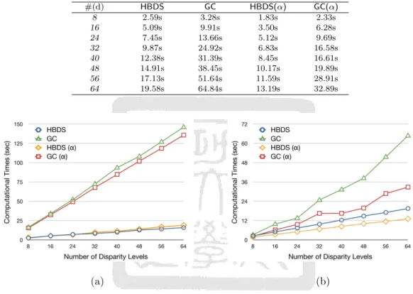
(11) List of Tables 2.1. Efficiency comparison for testing set containing multilayer disparity map. . 28. 2.2. Efficiency comparison for testing set containing gradient disparity map. . . 28. 2.3. Efficiency comparison for real stereo images. . . . . . . . . . . . . . . . . . . 29. 2.4. Comparison of bad pixel rate in GC and HBDS. . . . . . . . . . . . . . . . 30. 2.5. Comparison of bad pixel rate in conventional disparity refinement methods.. 2.6. Comparison of bad pixel rate in other occlusion boundary handling methods. 34. 3.1. Experimental results for 28 subjects under ideal conditions. . . . . . . . . . 53. 3.2. Distance errors (cm) of 3D positions estimated under different lighting conditions. . . . . . . . . . . . . . . . . . . . . . . . . . . . . . . . . . . . . . . 55. 3.3. Accuracy rates (%) of estimated results under different lighting conditions.. 3.4. Experimental results for various degrees of camera shift. . . . . . . . . . . . 57. 4.1. Errors of intersection angles between the constructed half-plane pairs for the stacked box image set. . . . . . . . . . . . . . . . . . . . . . . . . . . . . 72. 4.2. Errors of intersection angles between the constructed half-plane pairs for the Aerial Views I image set. . . . . . . . . . . . . . . . . . . . . . . . . . . 74. 4.3. The comparison of the computational cost between our method and Baillard’s method for the stacked box image set. . . . . . . . . . . . . . . . . . . 74. 4.4. The comparison of the computational cost between our method and Baillard’s method for the Aerial Views I image set. . . . . . . . . . . . . . . . . 74. x. 33. 56.

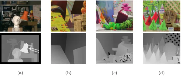
(12) List of Figures 2.1. Disparity structure used in graph cut algorithm. . . . . . . . . . . . . . . . 12. 2.2. Bilateral disparity division. . . . . . . . . . . . . . . . . . . . . . . . . . . . 14. 2.3. Hierarchical disparity structure. . . . . . . . . . . . . . . . . . . . . . . . . . 14. 2.4. (a) Left image of Teddy. (b) Ground truth disparity map. (c) Disparity histogram of the ground truth disparity map. (d) Rough disparity map. (e) Disparity histogram of the rough disparity map. . . . . . . . . . . . . . 20. 2.5. Two typical situations in which Otsu’s thresholding method fails to find the optimal break point: (a) bimodal case with different variances and (b) unimodal case. . . . . . . . . . . . . . . . . . . . . . . . . . . . . . . . . . . 21. 2.6. Typical example of foreground fattening effect. . . . . . . . . . . . . . . . . 22. 2.7. (a) Reference image. (b) Estimated disparity map. (c) Segmentation of the reference image. (d) Disparity edges. (e) Combination of disparity edges and segments. (f) Detected fattening regions. . . . . . . . . . . . . . . . . 23. 2.8. (a) Original disparity map. (b) Fattening regions. (c) Refined disparity map by Gu’s method. (d) Refined disparity map by proposed MDC method. 25. 2.9. First synthetic stereo testing image set. (a) Left image L. (b) Eighth right image R8 . (c) Ground truth disparity map. . . . . . . . . . . . . . . . . . . 27. 2.10 Second synthetic stereo testing image set (a) Left image L′ . (b) Eighth right image R′ 8 . (c) Ground truth disparity map. . . . . . . . . . . . . . . 27 2.11 Computational time comparisons for (a) synthetic testing image set containing multi-layer disparity map and (b) synthetic testing image set containing gradient disparity map. . . . . . . . . . . . . . . . . . . . . . . . . . . . . . 28 2.12 Four benchmark stereo images (upper) and corresponding ground truths (lower). (a) Tsukuba. (b) Venus. (c) Teddy. (d) Cones. . . . . . . . . . . . 29 2.13 Disparity maps and fattening regions in (a) Tsukuba, (b) Venus, (c) Teddy, and (d) Cones. . . . . . . . . . . . . . . . . . . . . . . . . . . . . . . . . . . 31 2.14 Refined disparity maps obtained by (a) 2DBF, (b) 2DBF+FFD, (c) 3DBF, (d) 3DBF+FFD, (e) WMF, and (f) WMF+FFD. . . . . . . . . . . . . . . 33 2.15 (a) Disparity map estimated by HBDS+MDC. (b) Corresponding disparity error. (c) Disparity map estimated by ASW. (d) Corresponding disparity error. (e) Disparity map estimated by cross-based method. (f) Corresponding disparity error. . . . . . . . . . . . . . . . . . . . . . . . . . . . . . . . 34. xi.

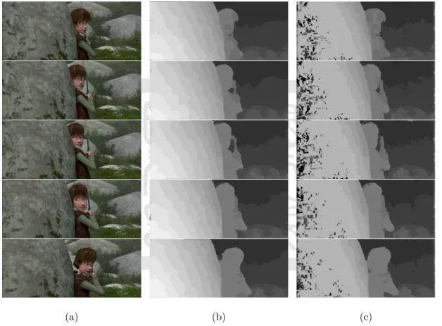
(13) 2.16 Experimental results obtained for real-world scenes. . . . . . . . . . . . . . 36 2.17 The experimental results of “Boy”: (a) left images, (b) disparity maps produced by HBDS+MDC, and (c) disparity maps produced by cross-based support window method. . . . . . . . . . . . . . . . . . . . . . . . . . . . . 37 2.18 The experimental results of “Little Dino”: (a) left images, (b) disparity maps produced by HBDS+MDC, and (c) disparity maps produced by crossbased support window method. . . . . . . . . . . . . . . . . . . . . . . . . 38 3.1. System flowchart of 3D localization approach. . . . . . . . . . . . . . . . . . 39. 3.2. (a) Captured image. (b) Image following skin-color segmentation. (c) Extracted edge contour of back. . . . . . . . . . . . . . . . . . . . . . . . . . . 42. 3.3. Schematic illustration of correspondence detection in CECT algorithm. Note that the blue line is the epipolar line corresponding to point c𝐿 , and the intersection point c𝑅 is the correspondence of c𝐿 . . . . . . . . . . . . . . 42. 3.4. (a) Sampling points along contour extracted from left image. (b) Corresponding points obtained along contour extracted from right image. . . . . 44. 3.5. An example of the triangle barycentric coordinates system. . . . . . . . . . 45. 3.6. Correspondence locating process. Note that the points in the right image with different colors (shapes) represent candidate correspondences estimated using different corresponding triangle pairs. . . . . . . . . . . . . . 49. 3.7. Schematic illustration of the vision-based robotic massage machine. . . . . . 50. 3.8. Unit of measurement in Traditional Chinese Medicine: “cun”.. 3.9. Captured back images of eight different subjects.. . . . . . . . 51. . . . . . . . . . . . . . . 52. 3.10 Captured back images of subject exposed to light from three different directions: (a) top-left (b) top-center and (c) top-right. . . . . . . . . . . . . 54 3.11 Mis-segmented back contour under unbalanced lighting conditions: (a) subject exposed to light from top-right; (b) corresponding segmentation result. . . . . . . . . . . . . . . . . . . . . . . . . . . . . . . . . . . . . . . . . . . . 54 3.12 Captured images given camera shifts of (a) 0 cm, (b) 4 cm, (c) 7 cm, and (d) 14 cm, respectively. . . . . . . . . . . . . . . . . . . . . . . . . . . . . . 57 4.1. System overview. . . . . . . . . . . . . . . . . . . . . . . . . . . . . . . . . . 58. 4.2. One-parameter family of half-planes spanned by 3D line L: (a) half-plane parameterized by angle 𝜇; (b) half-plane parameterized by feature point X.. xii. 60.

(14) 4.3. (a) Experimental image, rℎ is the half-plane to be bounded, r1 ∼ r3 are the nearby half-planes, and l1 ∼ l3 are the obtained fixed lines. (b) The possible fixed points around rℎ . (c) Hough accumulator array. . . . . . . . 65. 4.4. Geometry of fixed line and fixed point for 𝜋𝑟 and 𝜋ℎ . . . . . . . . . . . . . . 65. 4.5. Schematic illustration of the region-extension process via feature points. . . 67. 4.6. Practical example of region-extension process. . . . . . . . . . . . . . . . . . 67. 4.7. Merging the coplanar extended half-planes 𝜋(L) and 𝜋(L0 ). . . . . . . . . . 68. 4.8. Consecutive images of stacked camera boxes. . . . . . . . . . . . . . . . . . 70. 4.9. Reconstruction results obtained for stacked-box scene: (a) 3D wire-frame model (b) the half-planes associated with 3D lines (c) detected feature points and (d) grouped coplanar regions. . . . . . . . . . . . . . . . . . . . 71. 4.10 Reconstructed 3D model of stacked-box arrangement viewed in three directions. . . . . . . . . . . . . . . . . . . . . . . . . . . . . . . . . . . . . . . . . 71 4.11 The indices of planes used for accuracy evaluation: (a) stacked-box and (b) Aerial Views I. . . . . . . . . . . . . . . . . . . . . . . . . . . . . . . . . . . 72 4.12 Images in the Aerial Views I datasets. . . . . . . . . . . . . . . . . . . . . . 72 4.13 Reconstructed 3D model of Aerial Views I dataset observed from different views. . . . . . . . . . . . . . . . . . . . . . . . . . . . . . . . . . . . . . . . 73. xiii.

(15) Chapter 1 Introduction. In the past decade, the rapid development in the multiple view computer vision techniques has brought lots of conveniences to our daily life. Comparing to mono view, multiple view provides three significant advantages, e.g., 3D experience, depth information and larger view coverage. For example, with recent advances in 3D display technology, 3D viewing is becoming an achievable reality. The 3D display system provides the viewer with left/right images which are taken by a set of calibrated stereo camera. The realistic 3D viewing experience comes from the parallax between the stereo images seen in the viewer’s left eye and right eye, respectively. Besides, by exploiting the geometric information and the correspondences from the stereo camera, the 3D positions and depth information of the world points can be easily measured using the stereoscopic 3D localization technique. Furthermore, recent image-based 3D reconstruction approaches provide a convenient way to automatically generate highly realistic 3D models of real scenes using the images taken from multiple viewpoints [1–4]. The realistic 3D models are widely used in many computer-based event simulation and visualization, e.g., flight simulators, video games, augmented reality, 3D visual maps and so forth. In this thesis, we investigate the techniques of depth estimation from stereo views and 3D reconstruction from multiple views. First, for estimating dense depth map, an efficient and accurate graph cut based stereo matching method is developed. Second, a specialized stereoscopic 3D localization technique is designed for locating the points on featureless human back. Third, a method for efficiently reconstructing piecewise 3D planar models from multiple views is proposed.. 1.

(16) Depth Map Estimation from Stereo View In realizing 3D display systems, a knowledge of the disparity map, which contains depth information of the scene, between the stereo images in the viewing content is essential. For example, the free viewpoint television (FTV) technique offers the opportunity for a variable viewpoint by means of a DIBR (depth-image-based rendering) approach [5–7], in which one view and one disparity map are used to synthesize the images from other viewpoints. The disparity map provides essential spatial cues for allocating the image pixels in such a way as to accurately reproduce the depth relations of the different objects in a scene when viewed from different perspectives. The quality of the rendering images is fundamentally dependent on the accuracy of the disparity information. A high quality disparity map is also essential in improving the efficiency of 3D video coding schemes such as MVC (multiview video coding), MVD (multiview video plus depth) and LDV (layered depth video) [8–10]. Thus, the problem of improving the accuracy and efficiency of the disparity estimation process is an important and ongoing topic in the 3D technology field. The disparity estimation problem involves finding the correspondence of each pixel between two images. According to the taxonomy given in [11], the disparity estimation methods can be categorized as either local methods or global optimization methods, depending on the manner in which the disparity is computed. Local methods determine the disparity using the statistical correlation between the colors or texture patterns within a local support window [11–13]. Such methods consider only local information, and therefore have a low computational complexity and a short runtime. However, due to the ambiguity of the local information, local methods cannot ensure the smoothness of the object surfaces or preserve the discontinuities at the object boundaries. Global optimization methods treat the disparity assignment problem as a problem of minimizing a global energy function comprising a measurement of the local data and an additional smooth constraint for neighboring pixels. The smooth constraint is designed to retain the disparity smoothness of the pixels in the same region while simultaneously improving the estimation accuracy at the discontinuous object boundaries [11,14–20]. Various methods for solving the. 2.

(17) global energy minimization problem using a Markov Random Field (MRF) representation of the disparity energy function have been proposed. Broadly speaking, such methods can be classified as either graph cut (GC) methods [16–18] or belief propagation methods [19,20]. GC methods obtain the minimal energy solution by applying a min-cut/max-flow algorithm to the energy flow structure derived from the MRF graph. Meanwhile, belief propagation methods minimize the energy function by iteratively passing messages from current node to neighboring nodes in the MRF graph. Generally speaking, global methods achieve a higher disparity estimation accuracy than local methods, and therefore result in a better preservation of the object boundaries and an improved smoothness of the object surfaces [11]. Tappen and Freeman [21] compared the estimation performance of belief propagation methods and graph cut methods, respectively, and concluded that graph cut methods yield smoother disparity results. Thus, graph cut methods can be regarded as the optimal solution for disparity estimation when the quality of the estimation results is the primary consideration. Although graph cut methods yield a highly accurate disparity map, the optimization process is very time-consuming. Furthermore, the time cost increases exponentially with the size of the graph structure. Consequently, several approaches have been proposed for reducing the computational cost by simplifying the graph [22–25]. Segment-based methods such as those proposed in [22,23] use segmented regions rather than image pixels as the smallest unit for disparity assignment purposes. As a consequence, the number of vertices in the graph is reduced and the efficiency correspondingly improved. Segment-based approaches assume that all of the pixels in the same segment have the same disparity. However, if a segment contains a slant or curved surface, i.e., the segment contains pixels with a gradually varying depth and therefore different disparities, the segment will be incorrectly assigned with a single disparity. Moreover, if the image is not segmented properly, i.e., the segments contain multiple objects, these objects will also be incorrectly assigned with a single disparity in the estimation process. Lombaert et al. [24] used an image pyramid structure to improve the efficiency of the disparity estimation process. In the proposed approach, a rough disparity map was computed using the lowest image. 3.

(18) resolution level, and the disparity results were then repeatedly upsampled with a proper refinement to the next-highest level until the top level was reached. However, the original downsampling process causes many of the image details to be lost in the lowest resolution image. As a result, significant errors are generated and propagated in the upsampling process. Consequently, the improved estimation efficiency is obtained at the expense of a lower accuracy. Zureiki et al. [25] simplified the graph structure by considering only a few potential disparities of each pixel when constructing the graph. However, limiting the number of disparity levels inevitably increases the coarseness of the disparity map. In other words, a tradeoff is required between the efficiency of the estimation process and the quality of the disparity map. To resolve the information loss problem in the disparity estimation methods presented in [22–25], the present study proposes a Hierarchical Bilateral Disparity Structure (HBDS) algorithm which not only reduces the computational complexity of the estimation process, but also improves the accuracy of the disparity map. In the proposed algorithm, all the disparity levels in the image are divided hierarchically into lower level bilateral disparity structures until the finest disparity level is obtained. Within each bilateral structure, the disparity set is split into two subsets, namely the foreground subset and the background subset, respectively, in accordance with a pre-determined break point. The image pixels are then assigned to the appropriate subset using a graph cut algorithm. The hierarchical partitioning process changes the original disparity structure. Thus, a specialized energy function is proposed containing a new data term and a new smooth term. In partitioning the bilateral structures, the location of the break point has a key effect on the results of the foreground-background object separation process. If the break point is inappropriately determined, e.g., at a disparity within a foreground object in the scene, part of the object will be erroneously assigned to the background. In other words, the object will be divided into two objects; namely one foreground object and one background object. To resolve this problem, a disparity histogram-based thresholding method is applied to the pre-calculated rough disparity distribution of the stereo image in order to determine the optimal break point position. Since the graph cut process in HBDS involves only two levels, the computational com-. 4.

(19) plexity is significantly reduced. Moreover, due to the bilateral divisioning process, the number of active pixels decreases in the lower levels of the hierarchical structure, and consequently, the computational cost of the estimation performance is further reduced. During the estimation process, the HBDS algorithm takes account of all the available information (i.e., the full-resolution image pixels and the whole disparity range). As a result, the problem of information loss inherent in the graphsimplification methods presented in [22–25] is avoided. In other words, HBDS not only achieves a high computational efficiency, but also maintains the quality of the disparity map. In performing disparity estimation, a “foreground fattening” effect commonly occurs in which the background regions near the boundaries between objects at different depths in the image are erroneously assigned to the foreground [11,26,27]. In the present study, this problem is addressed by detecting the fattening regions in the disparity map and then recovering the corresponding disparities. In the proposed approach, the fattening regions are detected by checking whether or not the edges in the disparity map coincide with the object boundaries in the reference image. In the subsequent recovery stage, the disparities of the fattening regions are recovered using a modified form of the disparity calibration method [28]. In the modified disparity calibration (MDC) method, the disparities are determined using only the reliable neighboring pixels rather than all the neighboring pixels. Consequently, a more accurate refinement result is obtained than that achieved using the original disparity calibration method.. Stereo-based 3D Localization on the Texture-less Human Back In stereoscopic 3D localization, the 3D position of a world point is determined from the corresponding image points captured by two calibrated cameras. However, even small errors in the correspondences of the captured image points result in a significant error in the estimated 3D position. Therefore, when using the stereoscopic 3D localization approach, accurate techniques for identifying the correspondences in the left and right images are required.. 5.

(20) Many correspondence searching methods have been proposed in the past decade [29–34]. Some of these methods locate the correspondences directly by means of distinct markers placed on the subject [29,30], while others process various features of the image contents, such as the intensity, color or texture [31–34]. Although both methods produce excellent results in most situations, marker-based methods are impractical for back massage machines designed for self-use. Accordingly, marker-less approaches are widely preferred. Existing marker-less methods depend on the similarity measurement or pattern matching of distinctive and discriminative features in the images, such as SIFT descriptor [33] or CCH descriptors [34]. However, the skin on the human back is generally smooth, texture-less and lacking in distinguishable features. Consequently, marker-less methods are generally unable to detect reliable correspondence points in the stereo images of the human back. Even though the human back is generally smooth and texture-less, a few salient features such as moles, shadows and the edge contour nevertheless exist. These features are far more remarkable than the rest of the human back, and therefore provide a reliable foundation for correspondence searching. Accordingly, in the stereoscopic 3D localization technique proposed in this study, these distinctive features are used to identify reliable correspondences, and the reliable correspondences are then used as a reference for computing the correspondences of the featureless points. In the proposed approach, the edge contour is chosen as the primary salient feature for locating further correspondences since of all the salient features which can be extracted from the captured images of the human back, the edge contour is the most distinguishable and stable. Furthermore, all of the points which are to be localized lie on the human back, and thus the corresponding image points are all restricted to the region enclosed by the edge contour. The corresponding relations among the edge contours extracted from the left and right images, respectively, are established by applying the epipolar constraint in stereovision [35] and are treated as foundational correspondences. The points within the contour are then described according to these foundational correspondences using the Triangle Barycentric Coordinates (TBC) system [36]. The TBC descriptor enables the coordinates of any point to be efficiently and correctly transformed between two corresponding reference tri6.

(21) angles formed by any three foundational correspondences. As a result, it provides an ideal means of computing the correspondences of the featureless points on the human back given a knowledge of the foundational correspondences. The proposed scheme is designated as Correspondences from Epipolar geometry and Contours via Triangle barycentric coordinates (CECT). Compared to existing stereoscopic 3D localization schemes, CECT achieves a more efficient and robust identification of the correspondences on the human back by combining the respective advantages of content information (edge contours) and geometric information (epipolar constraint and TBC descriptor). The proposed 3D localization approach is applied to a newly developed visionbased interactive massage machine for human back. The massage machine comprises a stereo camera and a three-axis robotic arm. The stereo camera captures two images of the user’s back, which are then used to assess the user’s body shape and to determine the 3D coordinates of the specific point for massage. The robotic arm then moves to the appropriate coordinates and carries out the selected type of massage therapy. In addition, one of the captured images is displayed to the users and regarded as the interface for interactively determining the points for massage.. 3D Reconstruction of Planar Models from Multiple Views Most the man-made objects, such as buildings, vehicles, furniture, and so forth are composed of multiple planar facades or facets, and thus reconstructing the planar facades or facets in a realistic and accurate manner is essential in reproducing a life-like representation of the real-world scene. Many studies on image-based reconstruction have been proposed over the past decade. In general, these systems exploit the geometric properties of the real-world planes, such as vertical facades [4,37], horizontal planes [38], rectangular structures [39] and symmetry-based structures [40], or utilize a simple 3D wire-frame approach without attempting to verify the actual contents of planar regions [41,42]. More recently, some novel studies focus on reconstructing the models of entire city scenes [43,44], while some focus on 3D reconstruction from single image [45,46].. 7.

(22) Recent studies have shown that reconstruction systems based on inter-image homographies provide a particularly powerful technique for reconstructing models of real-world scenes containing planar regions [1,2,47,48]. For example, Baillard et al. [1] presented a method for reconstructing 3D models of buildings utilizing an inter-image homography technique and the concept of “half-planes”, namely a family of 3D planes rotating about a single 3D line. In [1], the half-plane was parameterized by the coordinates of the 3D line and the angle of rotation of the plane about the 3D line. Given the 3D borderline of a world plane, the correct half-plane, i.e., the halfplane corresponding to this world plane, was determined by searching through all the possible half-planes and by comparing the similarities of the regions projected by the half-plane between images. However, whilst this approach enhances the quality of the reconstruction results, the exhaustive search of the half-planes incurs a significant computational cost. In order to resolve this problem, the current study proposes a new half-plane parameterization method. Without loss of generality, an assumption is made that each correct half-plane contains at least one feature point, and thus the half-planes can be parameterized by the salient feature points distributed around the 3D line rather than searching every possible angle of rotation about the 3D line. Thus, the magnitude of the search process is reduced since it is necessary only to consider the salient feature points rather than 180 different angles of rotation. The complexity of the search process is further reduced by the imposition of two constraints, namely a coplanar constraint and a region constraint. The region constraint restricts the range over which the feature points are searched, while the coplanar constraint ensure that the selected feature points are coplanar in the 3D world. The imposition of these two constraints ensures that the maximum number of the feature points considered in the search process is far less than 180, i.e., the angles of rotation considered in the approach proposed in [1], and thus the efficiency of the search process is significantly improved. In practice, the estimated half-plane does not cover the entire region occupied by the corresponding 3D plane in the real world. Furthermore, more than one halfplane may represent the same 3D plane. Thus, in order to extract the complete planar region, the reconstruction method proposed in this study extends the correct. 8.

(23) half-plane to its maximum extent, and then merges all the half-planes which represent the same world plane. In performing the region-extension process, the search region must first be properly bounded to avoid the requirement for an exhaustive search over the entire image. In [3], an approach was proposed for estimating the boundary between neighboring planes in stereo images by utilizing the characteristics of the fixed line which is the intersecting line of two world planes determined by their inter-image homographies. This method provides a convenient means of establishing the most likely boundaries of a half-plane, and is therefore used in the present study to bound the search range for the half-plane region-extension process. In general, region-extension methods extend the region of interest in the outward direction on a pixel-by-pixel basis [1]. However, such an approach incurs a considerable computational cost. Thus, in this study, the region-extension process is based on the use of coplanar feature points rather than pixels. Since the number of feature points within the bounded search region is far less than the total number of pixels, the proposed approach is considerably more efficient than conventional pixelby-pixel schemes. Once each half-plane has been enlarged to its maximum extent, the complete region of the corresponding real-world plane is constructed by merging all the extended half-planes which are both adjacent to on another and coplanar.. The remainder of this thesis is organized as follows. Chapter 2 introduces the proposed stereo matching method including the detailed description of the HBDS algorithm and the foreground boundary refinement mechanism. Chapter 3 presents the stereoscopic 3D localization method which contains the proposed CECT algorithm and its application to the robotic back massage machine. Chapter 4 describes the 3D reconstruction method of piecewise planar models comprising half-plane identification, extension and merging procedures. The corresponding experimental results are presented at the end of each chapter, respectively. Finally, chapter 5 provides smoe brief concluding remarks.. 9.

(24) Chapter 2 Disparity Estimation Using HBDS-based GC Algorithm with a Foreground Boundary Refinement Mechanism. 2.1. Disparity Estimation using the GC Method. Disparity estimation is the problem of finding the dense correspondences between the reference image and the target image along the scanlines. The 𝑥 coordinate displacement between each pair of matching points is defined as the “disparity”. The goal of the stereo matching process is to assign every pixel 𝑝 ∈ 𝒫 in the reference image with a disparity 𝑑𝑝 ∈ 𝒟, where 𝒟 is the set of all possible disparities. Generally, the overall disparity assignment needs to be piecewise smooth within the object boundaries and discontinuous at the object boundaries.. 2.1.1. Energy Function and Graph. The disparity estimation problem can be formulated as an energy minimization problem based on an appropriately defined energy function. Typically, the energy function 𝐸(𝑑) comprises a data term and a smooth term [16,49], i.e. 𝐸(𝑑) = 𝐸data (𝑑) + 𝐸smooth (𝑑).. (2.1). The data term 𝐸data represents the intrinsic data energy, which measures the degree of fit of the disparity assignment 𝑑 in accordance with the observed data. The data term has the form 𝐸data (𝑑) =. ∑︁ 𝑝∈𝒫. 10. 𝐷𝑝 (𝑑𝑝 ).

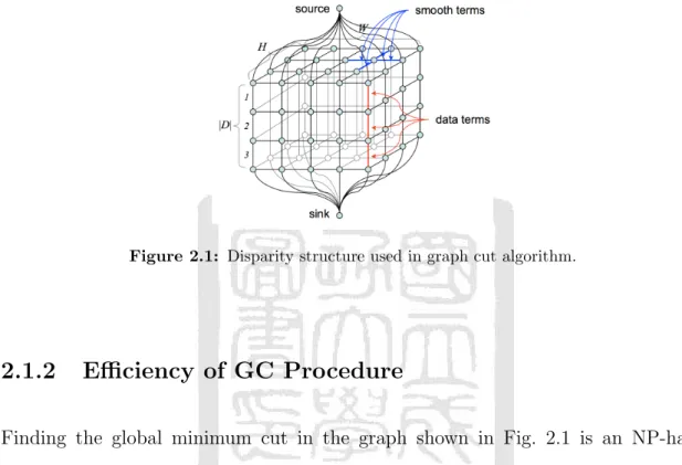
(25) where 𝐷𝑝 is the cost of assigning the disparity 𝑑𝑝 to pixel 𝑝. In the disparity estimation problem, 𝐷𝑝 is usually defined as the degree of dissimilarity between the reference pixel 𝑝 and its correspondence pixel 𝑝′ with disparity 𝑑𝑝 . The smooth term 𝐸smooth expresses the interaction between neighboring pixels. Specifically, it enforces the disparities of neighboring pixels to be smooth if the observed data are similar, while simultaneously ensuring the discontinuity of the disparities at the object boundaries. The smooth term has the form 𝐸smooth (𝑑) =. ∑︁. 𝑉{𝑝,𝑞} (𝑑𝑝 , 𝑑𝑞 ). {𝑝,𝑞}∈𝒩. where 𝒩 is the set of all neighboring pixel pairs, and 𝑉{𝑝,𝑞} is a function which attributes penalties to each pixel pair {𝑝, 𝑞} in accordance with the observed data and assigned disparities. In performing the disparity estimation process, 𝑉{𝑝,𝑞} is implemented as 𝑉{𝑝,𝑞} (𝑑𝑝 , 𝑑𝑞 ) = 𝑢{𝑝,𝑞} |𝑑𝑝 − 𝑑𝑞 | where the term 𝑢{𝑝,𝑞} represents the cost of assigning different disparities to the pair {𝑝, 𝑞}. As mentioned above, the disparity assignment should be smooth within objects and discontinuous at the object boundaries. Therefore, a large penalty 𝑢{𝑝,𝑞} should be assigned when neighboring pixels 𝑝 and 𝑞 are similar in order to prevent the disparities within the same object from being fragmented. The term |𝑑𝑝 − 𝑑𝑞 | in the penalty function has the effect of making the penalty 𝑉{𝑝,𝑞} proportional to the difference in the assigned disparities. In other words, the value of the smooth energy term increases when the disparity assignment passes through more disparity levels between the pair {𝑝, 𝑞}. To summarize, the global energy of the disparity labeling is defined as follows: 𝐸(𝑑) =. ∑︁ 𝑝∈𝒫. ∑︁. 𝐷𝑝 (𝑑𝑝 ) +. 𝑉{𝑝,𝑞} (𝑑𝑝 , 𝑑𝑞 ).. (2.2). {𝑝,𝑞}∈𝒩. Given the energy function defined in Eq. (2.2), a corresponding weighted graph with the dimensions of 𝑊 ×𝐻 ×|𝒟| can be constructed, where 𝑊 and 𝐻 are the width and height of the image and |𝒟| is the number of possible disparities (see Fig. 2.1). In the constructed graph, the weights of the vertical edges represent the energy associated with the data term; while the weights of the horizontal edges 11.

(26) represent the energy associated with the smooth term. A graph cut is a cutting surface between the source node and the sink node which separates the graph into upper and lower parts. The sum of the weights of the cut edges represents the overall energy value obtained from Eq. (2.2). Therefore, minimizing the energy of Eq. (2.2) is equivalent to finding the minimum cut in the graph.. Figure 2.1: Disparity structure used in graph cut algorithm.. 2.1.2. Efficiency of GC Procedure. Finding the global minimum cut in the graph shown in Fig. 2.1 is an NP-hard problem. For a disparity estimation process involving |𝒟| disparity levels and |𝒫| image pixels, the computational complexity scales exponentially with the number of disparity levels. Boykov et al. [16] proposed an efficient approach for finding the approximate global minimum graph cut using two move algorithms, namely the 𝛼expansion algorithm and the 𝛼-𝛽-swap algorithms. In the proposed approach, the energy minimization process was accomplished via a series of iterative cycles. In each cycle, the 𝛼-expansion algorithm was applied to each individual disparity and the 𝛼𝛽-swap algorithm was applied to every pair of disparities. Thus, each cycle involved (︀ )︀ |𝒟| iterations of 𝛼-expansions and |𝒟| iterations of 𝛼-𝛽-swaps. It was shown in [16] 2 that the energy minimization process terminated in 𝑂(|𝒫|) cycles. In other words, the solution procedure has a computational complexity of 𝑂(|𝒫||𝒟|2 ). That is, the computational complexity scales with the square of the number of disparity levels rather than exponentially. However, even so, the computational cost still increases significantly as the number of disparity levels increases. 12.

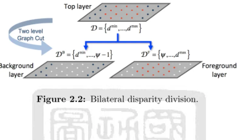
(27) 2.2. HBDS Algorithm. The HBDS algorithm is proposed for improving the efficiency of the disparity estimation process while simultaneously maintaining the quality of the disparity map. In HBDS, all disparity levels are divided hierarchically into multiple bilateral disparity structures until the finest disparity level is reached. Within each bilateral structure, the disparity set is split in accordance with a predetermined break point into two subsets, namely the foreground disparity set and the background disparity set. The image pixels are then assigned to the appropriate subset by minimizing the corresponding energy function using a graph cut algorithm. Each graph cut process involves just two levels. Thus, the computational complexity of each graph cut process is independent of the number of original disparity levels. Since HBDS decomposes the original multilevel disparity estimation problem into several bilateral disparity estimation problems, the overall computational complexity depends on the number of bilateral disparity estimation processes. In other words, the computational complexity varies linearly with the number of disparity levels.. 2.2.1. Proposed Disparity Structure. The basic concept of HBDS is to hierarchically decompose the original multilevel disparity estimation problem into a series of lower level bilateral disparity estimation problems. In each bilateral disparity estimation procedure, the current disparity set 𝒟 = {𝑑min , ..., 𝑑max } is divided into two subsets in accordance with a break point 𝜓. The subset containing the smaller disparities is regarded as the background subset and is labeled as 𝜆B , while the subset containing the larger disparities is regarded as the foreground subset and is labeled as 𝜆F . Accordingly, the bilateral disparity estimation problem is equivalent to that of finding the global labeling result 𝜆 which assigns each pixel 𝑝 ∈ 𝒫 with a bilateral label 𝜆𝑝 ∈ {𝜆B , 𝜆F } in such a way as to minimize the following energy function: 𝐸(𝜆) =. ∑︁ 𝑝∈𝒫. ∑︁. 𝐷𝑝 (𝜆𝑝 ) +. {𝑝,𝑞}∈𝒩. 13. 𝑉{𝑝,𝑞} (𝜆𝑝 , 𝜆𝑞 ).. (2.3).

(28) As shown in Fig. 2.2, the bilateral disparity estimation procedure separates the pixels in 𝒫 into a background layer 𝒫 B (containing all the pixels labeled as 𝜆B ) and a foreground layer 𝒫 F (containing all the pixels labeled as 𝜆F ). For each pixel 𝑝 with the label 𝜆B , the corresponding disparity 𝑑𝑝 is included in the set {𝑑min , ..., 𝜓−1}. By contrast, the disparity of each pixel labeled as 𝜆F is included in the set {𝜓, ..., 𝑑max }.. Figure 2.2: Bilateral disparity division.. The bilateral disparity estimation procedure is applied repeatedly to each separated layer to produce a hierarchical structure of bilateral layers with increasingly fine disparity sets. The top layer 𝒫 in this hierarchical structure contains all of the pixels in the reference image with the original disparity set {𝑑min , ..., 𝑑max }. As shown in Fig. 2.3, the initial bilateral disparity estimation process partitions 𝒫 into a foreground layer 𝒫 F and a background layer 𝒫 B . The bilateral disparity estimation procedure is then reapplied to separate 𝒫 F and 𝒫 B into their descendant bilateral layers, i.e., {𝒫 FF , 𝒫 FB } and {𝒫 BF , 𝒫 BB }, respectively. The partitioning procedure continues iteratively in this way until the divided disparity set reaches the finest disparity level.. Figure 2.3: Hierarchical disparity structure.. In the HBDS algorithm, the bilateral disparity estimation procedure described 14.

(29) above is implemented using the graph cut algorithm proposed in [16]. According to [16], the computational complexity of the graph cut algorithm is proportional to the number of pixels and the square of the number of disparity levels, i.e., 𝑂(|𝒫||𝒟|2 ). Since in HBDS, the number of labels used in each bilateral disparity estimation procedure is always equal to 2, the computational complexity of each graph cut algorithm is independent of the number of original disparity levels (i.e., 𝑂(|𝒫|)). HBDS continues to partition the original disparity set 𝒟 until the finest disparity subsets are obtained. Thus, a total of |𝒟| − 1 bilateral disparity estimation procedures are performed. As a result, the overall computational complexity of the HBDS disparity estimation process is equal to (|𝒟| − 1) × 𝑂(|𝒫|) (i.e., a complexity order of 𝑂(|𝒫||𝒟|)). Note that the number of pixels processed by the bilateral disparity estimation procedure reduces as the partitioning process proceeds to the lower disparity levels. As a result, the actual computational times of the lower layers are less than those of the higher layers.. 2.2.2. Specialized Energy Function for HBDS. Since the HBDS algorithm splits the original disparity set in a coarse-to-fine manner, the size of the processed disparity sets reduces as the estimation process continues. Consequently, the energy function used by the original graph cut algorithm cannot be applied. Accordingly, in this section, a new energy function specialized for HBDS is proposed.. Data Term The data term in the new energy function measures the cost of assigning the appropriate label to each pixel in accordance with the observed data. As described above, during each HBDS bilateral disparity estimation process, the disparity set 𝒟 is divided into a background subset 𝒟B and a foreground subset 𝒟F . Therefore, measuring the cost of assigning the label 𝜆𝑝 ∈ {𝜆B , 𝜆F } to a pixel 𝑝 is equivalent to measuring the cost of fitting the pixel 𝑝 to the corresponding disparity set {𝒟B , 𝒟F }.. 15.

(30) Accordingly, the problem of measuring the data terms 𝐷𝑝 (𝜆B ) and 𝐷𝑝 (𝜆F ) can be regarded as equivalent to that of choosing the most representative matching costs among the disparities in sets 𝒟B and 𝒟F , respectively. Since a smaller matching cost indicates a better assignment, the minimal matching cost obtained among the corresponding disparity set is adopted. The data term 𝐷𝑝 (𝜆𝑝 ) in the energy function utilized in HBDS is therefore defined as follows: ⎧ ⎪ ⎨ minF 𝑆(𝑝, 𝑑𝑝 ), 𝑑𝑝 ∈𝒟 𝐷𝑝 (𝜆𝑝 ) = ⎪ ⎩ min 𝑆(𝑝, 𝑑𝑝 ), 𝑑𝑝 ∈𝒟B. if 𝜆𝑝 = 𝜆F if 𝜆𝑝 = 𝜆B. (2.4). where 𝑆(𝑝, 𝑑𝑝 ) is the matching cost associated with the pixel 𝑝 and the disparity 𝑑𝑝 . From Eq. (2.4), it is seen that for 𝜆𝑝 = 𝜆F , the data term is determined by the minimal matching cost 𝑆(𝑝, 𝑑𝑝 ) found in the foreground disparity set 𝒟F . Similarly, for 𝜆𝑝 = 𝜆B , the data term is determined by the minimal matching cost 𝑆(𝑝, 𝑑𝑝 ) found in the background disparity set 𝒟B .. Smooth Term The smooth term in the energy function should enforce the disparities of neighboring pixels to be smooth if the observed data are similar, but should ensure that the disparities are discontinuous at the object boundaries. Accordingly, in performing bilateral disparity estimation, the smooth term can be designed as 𝑢{𝑝,𝑞} Δ(𝜆𝑝 , 𝜆𝑞 ), in which 𝑢{𝑝,𝑞} represents the penalty incurred when assigning different labels to neighboring pixels 𝑝 and 𝑞. If the two pixels are similar, i.e., they may belong to the same object and are likely to have the same label, 𝑢{𝑝,𝑞} should have a large value in order to prevent the pixels from receiving different labels during the estimation process. Conversely, if the two pixels are dissimilar, i.e., they most likely belong to different objects, the value of 𝑢{𝑝,𝑞} should be small in order to increase the likelihood of the pixels receiving different labels. In other words, the value of 𝑢{𝑝,𝑞} is inversely related to the similarity between 𝑝 and 𝑞. In practice, 𝑢{𝑝,𝑞} is generally implemented using the following decreasing function 𝑢{𝑝,𝑞}. {︀ }︀ min |𝐼𝑝 − 𝐼𝑞 |, 𝜏 = (𝑢min − 𝑢max ) + 𝑢max 𝜏 16.

(31) where 𝐼𝑝 and 𝐼𝑞 are the intensity values of pixels 𝑝 and 𝑞, respectively, and 𝜏 is a constant used to truncate and normalize the absolute difference value. In addition, the parameters 𝑢max and 𝑢min are two positive constants indicating the maximal and minimal penalties, respectively. In performing the disparity estimation process, the term Δ(𝜆𝑝 , 𝜆𝑞 ) is used to indicate whether or not pixels 𝑝 and 𝑞 are assigned with the same labels. ⎧ ⎨ 0, Δ(𝜆𝑝 , 𝜆𝑞 ) = ⎩ 1,. if 𝜆𝑝 = 𝜆𝑞. .. if 𝜆𝑝 ̸= 𝜆𝑞. In HBDS, the size of the divided disparity sets decreases from top to bottom. Thus, the effects of the smooth penalties incurred when assigning different labels to the neighboring pixels should be relative to the size of the corresponding disparity set. Consequently, the smooth penalty in HBDS is multiplied by an additional factor to take into account the size of the current disparity set 𝑉{𝑝,𝑞} (𝜆𝑝 , 𝜆𝑞 ) = 𝑢{𝑝,𝑞} Δ(𝜆𝑝 , 𝜆𝑞 ). |𝒟* | 2. (2.5). where |𝒟* | is the size of the disparity set in the current layer. Note that the term |𝒟* |/2 in Eq. (2.5) represents the average disparity difference to be passed through when assigning the different bilateral labels. It should be noted that |𝒟* |/2 has a larger value in the higher layers of the HBDS structure than in the lower layers due to the gradual reduction in size of the disparity sets as the partitioning process proceeds. Therefore, the bilateral disparity estimation which takes place at the higher layers yields a smoother result and tends to preserve the complete object regions due to the relatively stronger emphasis in the energy function on the smooth penalty. Conversely, in the lower layers, the bilateral disparity estimation process segments the scene in more detail due to the weaker emphasis on the smooth penalty. In other words, the HBDS algorithm performs a coarser disparity segmentation in the higher layers of the HBDS structure and a finer disparity segmentation in the lower layers.. 17.

(32) Matching Cost The matching cost function 𝑆(𝑥, 𝑦, 𝑑), which determines the data term, measures the degree of fit between the reference pixel 𝑝(𝑥, 𝑦) and the target pixel 𝑝′ (𝑥−𝑑, 𝑦) by comparing the observed features, e.g., the intensity, color or texture. The HBDS algorithm utilizes the matching cost function proposed in [50], which utilizes both the color features and the texture features to compute the matching cost. The cost function has the form (︁. )︁ (︁(︀ )︁ )︀ 𝑆(𝑥, 𝑦, 𝑑) = 𝑤(𝑥, 𝑦) × 𝑇 (𝑥, 𝑦, 𝑑) + 1 − 𝑤(𝑥, 𝑦) × 𝐶(𝑥, 𝑦, 𝑑). (2.6). where 𝐶(𝑥, 𝑦, 𝑑) is the matching cost of color feature, 𝑇 (𝑥, 𝑦, 𝑑) is the matching cost of texture feature, and 𝑤(𝑥, 𝑦) is a weighting ratio used to determine the relative importance of the texture features. Since the texture information is more distinguishable in the regions of the image with obvious edges, HBDS uses the normalized edge gradient value at 𝑝(𝑥, 𝑦) as the weighting ratio. In practical implementations, the edge gradient values are obtained by applying Sobel edge filter to the reference image. The color feature matching cost 𝐶(𝑥, 𝑦, 𝑑) is implemented using the linearly interpolated intensity function proposed in [51] 𝐶(𝑥, 𝑦, 𝑑) =. min{𝐶𝑓 (𝑥, 𝑦, 𝑑), 𝐶𝑟 (𝑥, 𝑦, 𝑑), 𝜂} . 𝜂. (2.7). In Eq. (2.7) the term 𝐶𝑓 (𝑥, 𝑦, 𝑑) measures the degree of fit between pixel 𝑝(𝑥, 𝑦) and pixel 𝑝′ (𝑥−𝑡, 𝑦), where 𝑡 lies in the disparity range [𝑑− 21 , 𝑑+ 12 ], and is computed as (︃ )︃ ∑︁ ⃒ ⃒ ⃒I𝛿 (𝑥, 𝑦) − I′𝛿 (𝑥 − 𝑡, 𝑦)⃒/3 𝐶𝑓 (𝑥, 𝑦, 𝑑) = min 1 ≤𝑡≤𝑑+ 1 𝑑− 2 2. 𝛿=𝑅,𝐺,𝐵. where I𝛿 (𝑥, 𝑦) represents the color value of 𝛿 ∈ {𝑅, 𝐺, 𝐵} at 𝑝(𝑥, 𝑦), and I′𝛿 (𝑥 − 𝑡, 𝑦) represents the color value at 𝑝′ (𝑥 − 𝑡, 𝑦). For symmetry, 𝐶𝑟 (𝑥, 𝑦, 𝑑) is also performed in the reverse direction in order to measure how well pixel 𝑝′ (𝑥−𝑑, 𝑦) fits back to pixel 𝑝(𝑡, 𝑦) with 𝑥− 12 ≤ 𝑡 ≤ 𝑥+ 21 . The corresponding equation is given as (︃ )︃ ∑︁ ⃒ ⃒ ⃒I𝛿 (𝑡, 𝑦) − I′𝛿 (𝑥 − 𝑑, 𝑦)⃒/3 . 𝐶𝑟 (𝑥, 𝑦, 𝑑) = 1min 1 𝑥− 2 ≤𝑡≤𝑥+ 2. 𝛿=𝑅,𝐺,𝐵. 18.

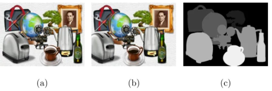
(33) Note that the constant 𝜂 in Eq. (2.7) is a truncated value used to reduce the influence of outliers and to normalize the value of the color matching cost within the range [0, 1]. Since the color matching cost is calculated in both the forward and the reverse directions with subpixel precision, the number of mismatches caused by noise in the stereo image pair is effectively reduced. The texture feature cost 𝑇 (𝑥, 𝑦, 𝑑) is implemented using the Normalized CrossCorrelation (NCC), which assesses the similarity between two pixels 𝑝 and 𝑝′ by inspecting their surrounding pixels within a bounding window 𝑊 )︀ (︀ )︀ (︀ ∑︀ I(𝑥, 𝑦) − 𝜇 × I′ (𝑥 − 𝑑, 𝑦) − 𝜇′ (𝑥,𝑦)∈𝑊 𝑁 𝐶𝐶(𝑥, 𝑦, 𝑑) = 𝑁 × 𝜎 × 𝜎′ where 𝜇 and 𝜎 denote the mean value and the standard deviation of the pixels within 𝑊 in the reference image, 𝜇′ and 𝜎 ′ denote the mean value and standard deviation of the corresponding pixels in the target image, and 𝑁 is the number of pixels within 𝑊 . The value of NCC ranges from −1 to 1, where a larger value indicates a better matching. Thus, the texture matching cost is obtained as 𝑇 (𝑥, 𝑦, 𝑑) =. 2.2.3. 1 − 𝑁 𝐶𝐶(𝑥, 𝑦, 𝑑) . 2. (2.8). Determining Optimal Break Point. The performance of the HBDS algorithm is fundamentally dependent on the value of the break point 𝜓 used to split the disparity set 𝒟 into the background and foreground subsets 𝒟B and 𝒟F . In general, a good background-foreground separation should result in an appropriate assignation of the scene objects to the bilateral layers in accordance with the scene composition and should prevent a single object at the same depth from being separated and assigned to two different layers. For illustration purposes, consider the stereo image set Teddy [52] shown in Fig. 2.4(a). The corresponding ground truth disparity map and disparity histogram are shown in Fig. 2.4(b) and (c), respectively. As shown in Fig. 2.4(c), the disparity histogram contains two distinct groups of pixels. This implies that the scene shown in Fig. 2.4(a) can be properly separated into two layers given the selection of an appropriate break point. Logically, the results presented in Fig. 2.4(c) suggest that 19.

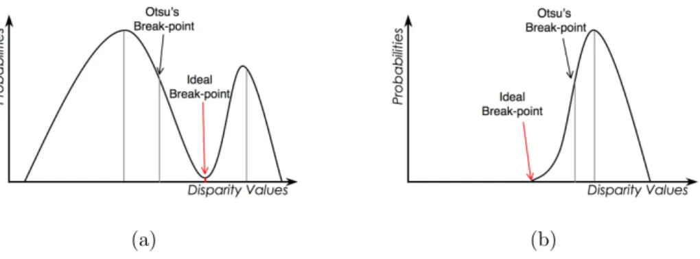
(34) (a). (b). (c). (d). (e). Figure 2.4: (a) Left image of Teddy. (b) Ground truth disparity map. (c) Disparity histogram of the ground truth disparity map. (d) Rough disparity map. (e) Disparity histogram of the rough disparity map.. the break point should be selected within the valley region between the two pixel groups. If the break point is specified in the middle of the foreground group (for example), part of the objects which properly belong to the foreground region of the image will be erroneously assigned to the background region. In general, to achieve a correct and balanced scene separation, the break point should be set at a point which divides the histogram into two main groups of pixels and contains the smallest number of pixels as possible. The thresholding method proposed by Otsu [53] finds the threshold value of 𝜓 in the range [𝑑min , 𝑑max ] which minimizes the within-class variance 𝜎𝑤2 (𝜓) = 𝜔F (𝜓)𝜎F2 (𝜓) + 𝜔B (𝜓)𝜎B2 (𝜓). (2.9). where 𝜔B and 𝜔F are the cumulative probabilities of the two groups separated by the threshold 𝜓 and 𝜎B and 𝜎F are the variances of these groups. Otsu’s thresholding method yields the statistically optimal solution for the break point if the two groups both have a Gaussian distribution. However, in practical situations, Otsu’s method has two significant drawbacks. First, according to the analysis presented in [54], when the difference between the within-class variances of the two groups is large, the threshold value is biased toward the group with the larger variance (see Fig. 2.5(a)). Second, it was shown in [55] that Otsu’s method usually fails to find a proper threshold if the distribution is unimodal or close to unimodal (see Fig. 2.5(b)). In other words, although Otsu’s method provides a threshold parameter value which enables the disparity histogram to be separated into two main groups, the threshold is not guaranteed to be located in the valley region between 20.

(35) (a). (b). Figure 2.5: Two typical situations in which Otsu’s thresholding method fails to find the optimal break point: (a) bimodal case with different variances and (b) unimodal case.. the two groups. Consequently, it is not suitable for the bilateral disparity estimation problem considered in the present study. In implementing the HBDS algorithm, the optimal value of the break point is determined by searching for the position with the lowest probability of pixel occurrence between 𝜇F and 𝜇B , which are the means of the two groups obtained via Otsu’s method. In other words, the optimal break point is determined as 𝜓 = arg min {𝑃T }. (2.10). 𝜇B ≤T≤𝜇F. where 𝑃T denotes the probability of pixel occurrence and is obtained from the disparity histogram at position T. Since the break point obtained from Eq. (2.10) is located at the position containing the fewest pixels between the two groups found by Otsu’s method, it is guaranteed that the bilateral disparity estimation process will avoid most of the erroneous segmenting situations in which an object at the same depth is segmented and assigned to different layers. Note that in practical implementation, a rough disparity map can be obtained using a simple Winner-Takes-All method from the matching cost volume computed before the optimization process. The rough disparity map provides an approximate indication of the disparity distribution of the stereo pair, and therefore allows an estimated disparity histogram to be obtained. Fig. 2.4(d) and (e) show the rough disparity map and the corresponding disparity histogram of the Teddy stereo pair.. 21.

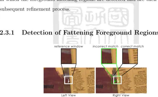
(36) 2.3. Disparity Refinement with Fattening Foreground Region Detection. In this section, the computed disparity map is further refined to remove the noises and to improve the precision at the object boundaries. Traditional disparity refinement methods, e.g. [28,56–58], achieve an effective refinement of the original disparity map by exploiting the information provided by the neighboring pixels. However, these methods are usually affected by a foreground fattening effect due to the window-based matching cost induced when computings the original disparity map [11,26,27]. Accordingly, this section proposes a disparity refinement mechanism in which the foreground fattening regions are detected and are then ignored in the subsequent refinement process.. 2.3.1. Detection of Fattening Foreground Regions. Figure 2.6: Typical example of foreground fattening effect.. In disparity estimation, a foreground fattening effect commonly occurs at the boundary between two objects at different depths when the background object has a homogeneous and repetitive pattern. Fig. 2.6 illustrates a typical example of the foreground fattening phenomenon. Consider point 𝑝 in the left view, located in the background region close to the boundary with the foreground region. Let the corresponding point in the right view be denoted as point 𝑝′ . Since the background region near the boundary in the right view is occluded by the foreground object, the pattern in the window centered on 𝑝′ is dissimilar to that in the reference window. Furthermore, since the homogeneous and repetitive patterns in the 22.

(37) (a). (b). (c). (d). (e). (f). Figure 2.7: (a) Reference image. (b) Estimated disparity map. (c) Segmentation of the reference image. (d) Disparity edges. (e) Combination of disparity edges and segments. (f) Detected fattening regions.. background region provide no distinctive features, the matching cost is dominated by the foreground region contained within the window. In such a situation, the incorrect matching point found when minimizing the matching cost usually has the same disparity as that of the nearby foreground object (e.g., point 𝑝′′ in Fig. 2.6). Therefore, the disparity estimation process erroneously assigns the foreground disparity to the background region near the boundary; causing the foreground region in the estimated disparity map to be larger than the actual foreground region. In the disparity estimation process, the edges in the disparity map represent the boundaries between objects located at different depths in the scene. If the disparities are correctly assigned, the disparity edges coincide with the corresponding object edges in the reference image. However, if the foreground fattening effect occurs, the edges of the fattening objects in the disparity map no longer match the corresponding edges in the reference image. Accordingly, in the foreground refinement mechanism proposed in this study, the fattening regions are detected by comparing the edges in the disparity map with the edges in the reference image. The disparity edges are obtained by applying the Canny edge detector [59] to the estimated disparity map. Fig. 2.7(a) and (b) show a typical reference image and the estimated disparity map, respectively. In order to determine the correct positions of the object boundaries, the reference image is partitioned into many small homogeneous regions (superpixels) using the segmentation technique proposed in [60]. (Note that this technique has the ability to avoid the under-segmentation problem, in which a single segment may contain multiple objects.) Fig. 2.7(c) shows the segmentation image results for the reference image in Fig. 2.7(a). Fig. 2.7(d) shows the disparity edges obtained from 23.

(38) the disparity map in Fig. 2.7(b). Having segmented the image, the coincidence (or otherwise) of the disparity edges with the segment boundaries is checked (see Fig. 2.7(e)). If a disparity edge lies on a segment, but does not fit the corresponding segment boundary, it is regarded as a fattening edge. The fattening edge divides the segment into two regions, i.e., the erroneous foreground fattening region and the background region. Since the fattening region is misassigned to the foreground, it has a larger disparity value than the neighboring background region. In other words, the region with the larger disparity value is detected as the fattening region. Fig. 2.7(f) shows the detected fattening regions in the disparity map shown in Fig. 2.7(b).. 2.3.2. Disparity Recovery. Once the fattening regions have been identified, the disparities within the image are recovered using a modified form of the disparity calibration method presented by Gu in [28]. In Gu’s method, the disparity values are calibrated in accordance with the disparity values of all the neighboring pixels within the supporting window. However, the erroneous disparity values in the fattening regions adversely affect the calibration results. Accordingly, in the proposed refinement mechanism, the fattening regions are excluded in order to enhance the accuracy of the calibrated disparity results. In implementing the modified disparity calibration (MDC) method, the calibrated disparity of pixel 𝑝 is determined by computing the supporting scores of all the possible disparities in {𝑑min , ..., 𝑑max } for pixel 𝑝 in accordance with the disparity values of all the reliable pixels within a window centered at 𝑝. Specifically, the supporting score of disparity 𝑑 for pixel 𝑝 is computed as Ω(𝑝, 𝑑) =. ∑︁. 𝑤(𝑝, 𝑞) × 𝐶(𝑞, 𝑑). (2.11). 𝑞∈W. where W represents the set of pixels in the supporting window. The function 𝑤(𝑝, 𝑞) in Eq. (2.11) measures the adaptive support-weight [61] between pixels 𝑝 and 𝑞 and therefore indicates the likelihood of the two pixels belonging to the same object. 𝑤(𝑝, 𝑞) considers both the color similarity of the two pixels and the spatial distance 24.

(39) between them, that is (︂ (︂ )︂)︂ Δ𝑐(𝑝, 𝑞) Δ𝑔(𝑝, 𝑞) 𝑤(𝑝, 𝑞) = exp − + 𝛾𝑐 𝛾𝑔 where Δ𝑐(𝑝, 𝑞) is the color distance between pixels 𝑝 and 𝑞, Δ𝑔(𝑝, 𝑞) is the spatial distance between pixels 𝑝 and 𝑞, and 𝛾𝑐 and 𝛾𝑔 are variables used to normalize the color and spatial distances, respectively. The term 𝐶(𝑞, 𝑑) in Eq. (2.11) is a binary decision function which indicates whether pixel 𝑞 has the disparity value 𝑑 while simultaneously excluding the pixels in the fattening regions. 𝐶(𝑞, 𝑑) is defined as ⎧ ⎨ 1, if 𝑑(𝑞) = 𝑑 and 𝑞 ∈ / fattening regions 𝐶(𝑞, 𝑑) = (2.12) ⎩ 0, else where 𝑑(𝑞) represents the disparity of pixel 𝑞. Significantly, the constraint defined in Eq. (2.12) ensures that only those pixels not in the fattening region are taken into account when calculating the supporting scores of the disparities. Finally, the disparity 𝑑′ which has the maximal supporting score is chosen as the recovered disparity value for pixel 𝑝, that is (︀ )︀ 𝑑′ = arg max Ω(𝑝, 𝑑) .. (2.13). 𝑑∈𝒟. Fig. 2.8(a) and (b) show a typical disparity map and the corresponding fattening regions, respectively. The refined disparity map produced by Gu’s method [28] is shown in Fig. 2.8(c), while the refined disparity map obtained using the method described above is shown in Fig. 2.8(d). It is seen that Gu’s method actually degrades the accuracy of the disparity map in some of the fattening regions (see the circled areas in Fig. 2.8(c)). By contrast, the refinement method proposed in this study improves the precision of the disparity map at the object boundaries.. (a). (b). (c). (d). Figure 2.8: (a) Original disparity map. (b) Fattening regions. (c) Refined disparity map by Gu’s method. (d) Refined disparity map by proposed MDC method.. 25.