On: 28 April 2014, At: 06:44 Publisher: Routledge
Informa Ltd Registered in England and Wales Registered Number: 1072954 Registered office: Mortimer House, 37-41 Mortimer Street, London W1T 3JH, UK
Transportation Planning and
Technology
Publication details, including instructions for authors and subscription information:
http://www.tandfonline.com/loi/gtpt20
A spatial and temporal bi
‐criteria
parallel
‐savings‐based heuristic
algorithm for solving vehicle routing
problems with time windows
Gwo‐Hshiung Tzeng a , Wen‐Chang Huang a
& Dusan Teodorovic b
a
Energy and Environmental Research Group and Institute of Traffic and Transportation , National Chiao Tung University , Taiwan, R.O.C.
b
Faculty of Transport and Traffic Engineering , University of Belgrade , Belgrade, Yugoslavia
Published online: 21 Mar 2007.
To cite this article: Gwo‐Hshiung Tzeng , Wen‐Chang Huang & Dusan Teodorovic (1997) A
spatial and temporal bi‐criteria parallel‐savings‐based heuristic algorithm for solving vehicle routing problems with time windows, Transportation Planning and Technology, 20:2, 163-181, DOI: 10.1080/03081069708717586
To link to this article: http://dx.doi.org/10.1080/03081069708717586
PLEASE SCROLL DOWN FOR ARTICLE
Taylor & Francis makes every effort to ensure the accuracy of all the information (the “Content”) contained in the publications on our platform. However, Taylor & Francis, our agents, and our licensors make no representations or warranties whatsoever as to the accuracy, completeness, or suitability for any purpose of the Content. Any opinions and views expressed in this publication are the opinions and views of the authors, and are not the views of or endorsed by Taylor & Francis. The accuracy of the Content should not be relied upon and should be independently verified with primary sources of information. Taylor and Francis shall not be liable for any losses, actions, claims, proceedings, demands, costs, expenses, damages, and other liabilities whatsoever or howsoever caused arising directly or indirectly in connection with, in relation to or arising out of the use of the Content.
substantial or systematic reproduction, redistribution, reselling, loan, sub-licensing, systematic supply, or distribution in any form to anyone is expressly forbidden. Terms & Conditions of access and use can be found at http://www.tandfonline.com/ page/terms-and-conditions
Photocopying permitted by license only license by Gordon and Breach Science Publishers Printed in Malaysia
A SPATIAL AND TEMPORAL BI-CRITERIA
PARALLEL-SAVINGS-BASED HEURISTIC
ALGORITHM FOR SOLVING VEHICLE
ROUTING PROBLEMS WITH TIME WINDOWS
GWO-HSHIUNG TZENG*,a, WEN-CHANG HUANGa and
DUSAN TEODOROVICb
aEnergy and Environmental Research Group and Institute of Traffic and Transportation, National Chiao Tung University, Taiwan, R.O.C.; bFaculty of
Transport and Traffic Engineering, University of Belgrade, Belgrade, Yugoslavia
(Received 25 June 1996; In final form 12 September 1996)
This paper proposes a spatial and temporal bi-criteria parallel-savings-based heuristic algorithm for solving vehicle-routing problems with time windows. The purpose of the algorithm is to reduce transportation costs and to satisfy the specific times, within time windows, which are required by customers. For evaluating the performance of the algorithm, two separate sets of time windows are created by generating data randomly. The test results reveal that both the preciseness and stability of the solutions perform much better than those based on the insertion method.
Keywords: Vehicle-routing problem; time windows; Bi-criteria; parallel savings; heuristic
algorithm
1. INTRODUCTION
Routing, scheduling and loading are prime factors that influence several costs in delivery systems. They represent the crux for the construction of a solution to the vehicle-routing problem with time windows. Typically, solutions are based on the well-understood traveling salesman problem (TSP). The objective is to minimise the total routing distance and to limit trips so as to pass by every customer point only once. This can be likened to the Hamiltonian cycle in
* Corresponding Author
163
graph theory. In the vehicle-routing problem (VRP), customers have a known demand for a service, and the total demand on the route cannot exceed the vehicle capacity. VRP, with the addition of loading limits, can be formed from TSP, and supplementary Hamiltonian cycles will be formed for all customers due to the loading limit. Therefore, the VRP looks for the shortest-routing distance to fulfill the customers requirements with a fleet of vehicles. Once the constraint of time windows is placed into VRP, it becomes a vehicle-routing problem with time windows (VRPTW). This means that every customer has a service-time interval (time window). Thus, we can see that VRPTW is actually an interdependent problem consisting of routing, scheduling and loading as the three major intertwining problems.
'Hard' and 'soft' windows can be respectively separated from time windows in VRPTW. The former, hard windows, refers to the time window constraint that allows no vehicle violation; the latter, soft windows, is the opposite case where time window constraints are put into the indices when searching for better solutions. This paper investigates the latter case.
In view of the features of vehicle fleet size and mix, we have a homo-geneous fleet and a heterohomo-geneous fleet. This paper deals with the problems of a homogeneous fleet, and the size of the fleet will depend on the number of tours.
If the characteristics of a network are considered in terms of connectivity, two types of network can be obtained, one complete and one incomplete. For the former, each of the customer points can be linked by a segment and vice versa. However, in the latter, once the transformation techniques have been applied to the data structure, one complete network can be formed. Whether the network is directional will be another important trait. With regard to the distance matrix, the possibility of forming either a symmetrical or an asymmetrical matrix will directly affect the data process. The items studied in this paper are for the non-directional complete network.
The structure of this paper is as follows: the next section reviews the liter-ature; the third section develops the spatial and temporal bi-criteria parallel-savings-based heuristic; the fourth section contains the test results; and the last section draws some conclusions.
2. LITERATURE REVIEW
One of the typical heuristic methods to find solutions to the VRP, the savings method, was developed by Clarke and Wright (1964), with the initial solution of servicing every node by a distinct vehicle. Then, upon satisfying the demands of two customers by the same vehicle, the savings will appear. These
savings are sorted in descending order. The original Clarke-Wright algorithm merges customers, taking into account the highest saving and existing vehicle capacity restrictions. There is a so-called sequential version and a concurrent version of this algorithm. The constraint of the former method is that the second tour can only be constructed after the completion of the first one, while the latter method follows strictly the savings index to contrive many tours (possibly just one). The superiority of one method over the other is still undecided (Golden, 1977; Mole and Jameson, 1976). Golden (1976) proposed the pathological analysis of the tour-contrivance method and attempted to show that higher stability is found in the sequential-contrivance method. If the techniques for finding solutions used in matching problems are applied, the results obtained from the pathological analysis put forward by Golden would not stand. Even though the savings method can be a way to find solutions to VRP, no in-depth consideration has ever been placed on the loading problem as the major key.
The parallel-savings-based heuristic put forward by Altinkemer and Gavish (1991) has used the management techniques of matching problems to combine tours endlessly so as to identify solutions to the VRP, in the hope that the arrangements of tours as a whole can be fully studied. Nevertheless, if the management techniques of matching problems alone are used, the loading limit is liable to be bypassed very soon, and solutions of inferior quality are most likely to be reached. In view of this, Altinkemer and Gavish suggested the notion of adding dummy points to control the violation speed of the loading limit. Therefore, the combination of the management techniques of matching problems and the notion of adding dummy points will be given dual func-tions: (1) to allow multiple combinations of loading and (2) to consider tour arrangements as a whole. Given such capabilities, the two major issues of the VRP, routing and loading, can be solved.
On the other aspect, Solomon (1986,1987), Golden et al. (1986) and Kolen
et al. (1987) tried many methods to solve the VRPTW. They concluded that
the insertion method achieved the highest degree of precision and stability in resolving solutions compared with all others, since the criteria it uses for seeking the better solutions are mainly space and time. The bi-criteria put forth by Van Landeghem (1988) to solve the VRPTW has applied the notion of scheduling. The purpose is to exhaust both the conventional means of routing, as well as the management techniques of scheduling, in finding a solution. However, the solutions to routing and scheduling in regard to the VRPTW fail to include loading combinations in their deliberations.
Given the significance of these three important issues, this paper proposes the concept of a spatial and temporal bi-criteria parallel-savings-based heuristic
to solve the VRPTW. The notation used is as follows, where N: the number of nodes in the problem; C: the vehicle capacity; g,-: the load to be delivered to node i; e,: the earliest allowed time point for beginning of service at node
i; /,•: the latest allowed time point for beginning of service at node i; and sp
duration of the service at node i.
3. THE SPATIAL AND TEMPORAL BI-CRITERIA
PARALLEL-SAVINGS-BASED HEURISTIC ALGORITHM
Three main points are included in this section: (1) the spatial and temporal bi-criteria saving index; (2) the parallel-savings-based heuristic; and (3) the algorithm of the spatial and temporal bi-criteria parallel-savings-based heuristic.
3.1. The Spatial and Temporal Bi-Criteria Saving Index
In terms of the spatial index, this study has employed the notion of a revised savings index by Yellow (1970), that is
sij = di0 + doj-gx dij (1) where sij is the savings value between point i and point j ; d[0 is the distance from delivery point / to depot; d^ is the distance between points / and j ; and
g is the route shape parameter.
In terms of the temporal index, the concept of "flexibility of scheduling" is presented in this paper and the overlapping of time windows is employed to see if it is beneficial to scheduling. Definitions of symbols are put forward to simplify the elaboration.
Entry window: the time window of the first customer being serviced after scheduling in a tour, indicated by (ea, la); where ea will be the starting point of the time window while la is the finishing point of the time window.
Exit window: the time window of the last customer being serviced after scheduling in a tour, indicated by (ev, /„); where ev will be the starting point of the time window while lv is the finishing point of the time window.
The time window of customer i: the initial time window of customer i yet to be scheduled, indicated by (e,-, /,-); where i ^ a, and i ^ v.
The service duration to customer /: the duration the vehicle stays at the customer point i, indicated by s,-.
Travel time from customer i to customer j : the routing time the vehicle spent on traveling from customer i to customer j , indicated by fy.
The maximal waiting time of vehicle: If the maximum tolerable waiting time of a vehicle at any one of the customer points is exceeded, such a customer will not be serviced (rendering an infeasible solution). It will be indicated by Max W.
Let us consider what is happening when service is done for customer i before customer j . In this case, the earliest and latest possible time points for beginning of service at node j are respectively equal to (e,- + si + tij) and
(/,- + Si + tij).
If the intersection of the two time windows (e,-+«,•+/,•_,-, /,•+•?,• + *,•_,•) and the time window (ej, /_,-) is not an empty set, it would be, Min(/,- + s,- + /,;-, lj) —
MaxO,- + si + tij, ej) > 0.
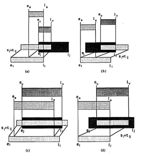
The entry and the exit windows are defined by the following relations: Entry window = (ea, la) = (Max(e,-, ej — ttj — st), Min(/,-, lj — ttj — st))
Exit window = (ev, lv) = (Max(e; + Si + tij, ej), Min(/,- + si + tij, lj))
as indicated in Figures l(a), (b), (c) and (d).
If the intersection is an empty set, and the waiting time is less than or equal to Max W, it would be:
0 < Max(e,- + st + ttj, ej) - Min(/,- + st + t{j, lj) < Max W ENTRY WINDOW = (ev, lv) = (/,-, /,-)
EXIT WINDOW = (ev, lv) = (eJt ej)
as indicated in Figure l(e).
If the intersection is an empty set and the corresponding waiting time has already exceeded the tolerable range, it would be, Max(e,- + S; + tij, ej) — Min(/,- + si + tij, lj) > Max W, as indicated in Figure 1 (f). In this case we will have an infeasible solution, without entry and exit windows.
Inequality e,- + s,- + tij > lj shows that customer j cannot be served after customer i. This case is shown in Figure l(g). The case is also characterized by the infeasible solution which is attributable to a shortage of entry and exit windows.
From the perspective of tour contrivance, the width of the entry and exit windows, which stands for the time window of the tour, is considered the key to scheduling in this study. When the intersection of the transformed time windows of time and space is not of an empty set, the tour width of either the entry or exit windows will be selected as the "flexibility of scheduling", with its index value to be the benefit item. When the intersection of the transformed time windows of space and time is an empty set and its waiting
I e i ! V (b) e si+ tU , a | I 1 l i
A
V / ei (c)FIGURE 1 Relationships of overlap in two time windows after the transformation of space and time.
time has not yet surpassed the tolerable range (Max W), the waiting time is chosen to respond to scheduling and the index value (flexibility of scheduling) now will be the item of cost (time). Thus, flexibility of scheduling F,;- =
Min(/,- + si + ttj, lj) - Max(e,- + 5,- + r,;-, e,) will be the index value while
Fij + Max W > 0.
Because of the differences in units between the distance index for better spatial routing and the time index for better temporal scheduling, the trans-formation techniques of a normalized linear scale are used in this paper, with an integrated index obtained from these two weighted factors, so that these two factors can be considered together. Moreover, both the negative and positive ideal solutions, acting as the extreme values for the linear scale of transformation, are employed on the grounds of iteration and of tackling an infeasible solution. Teodorovic, Kikuchi and Hohlacov (1991) have also used the TOPSIS method to obtain some kind of integrated index.
ea."a ev - l , S,+t MaxW "a,1 a v '" v (g) FIGURE 1 Continued
In terms of the distance index for better spatial routing,
SN'=
SiJ-
MinS11 M a x S - M i n S
where, SNij is the normalized value of Sty,
Max5 = 2 x Max{d,0} — g x Min{di;};
(2)
MinS = 2 x Min[dio} -gx Max{d,-,-};
In terms of the time index for better temporal scheduling,
= MaxW + F,7
ij MaxW + M a x F where, FNtj — F,7 will be the normalized value;
Fij = Min(/,- + si + Uj ,lj)- Max(e; + st + tu, ej) (4)
M a x F = Max{F,-,}.
ij
The weighting for the indices between the spatial and the temporal bi-criteria will be to combine the index for routing with that of temporal scheduling as one index:
SAL,7 = h x SNtj + (l-h)x FNU (5) where, SAL,7 = the indices of combining the spatial and the temporal
bi-criteria;
h = the weighting of the index of the importance for
spatial routing.
If the time window is ignored while h = 1, it will become the method to resolve conventional routing problems; if the saved routing distance is not considered and h = 0, it will be the method to resolve scheduling problems.
3.2. Parallel-Savings-Based Heuristic Algorithm
A savings method is conducted for the initial solution with one vehicle and one customer point, while the idea of a triangular inequality equation is then applied to narrow down the total routing distance of the initial solution. The method to reach the final solution would be attained at the end. During the contrivance of tours, only the linking of customer points to the depot will be taken into consideration, that is the combined benefits of the end-points. Therefore, the combined benefits of the two end-points, from the perspec-tive of each tour, alone have to be considered; in other words, the degree of each tour will constantly be two. Upon acquiring such characteristics, each tour can be taken as a point with two dimensions, and one fewer point will come from every merger for the entire network. With the trait of "degree of tour" constantly being two, as well as the needs of frequent merging oper-ations during tour contrivance, matching problems can be used to speed up tour contrivance, so that the benefits are considered comprehensively and the merging processes can be facilitated more efficiently. If the loading limit of the
VRP is shelved momentarily, it then becomes a TSP. The matching problem can then be used to lower the number of points of the network to half the size each time. Through iterating a matching problem, a Hamiltonian cycle can be obtained (if AT = 2").
Nonetheless, various situations are likely to occur if and only if matching problems are used to solve the vehicle routing problem. When the loading of all tours is greater than C/2, but far less than C, the heuristic algorithm can be used. As a result no more tour mergers are possible, and solutions are usually very far from optimum. To control the speed of the violation of the loading limit, the technique of adding dummy points proposed by Altinkemer and Gavish (1991) can be modified, so that the objective of parallel solutions can be obtained. Altinkemer and Gavish proposed to add a set of dummy nodes M,• to the network at each iteration i, with the idea of solving the rate at which tours are formed. Several qualifications are required for achieving this objective: (1) the dummy node must possess the traits of other actual nodes; (2) its quantity of necessity must be zero; (3) the additional node |Af,-| = 2 x (n — (i + 1) x T) — | V,_i |; where M,- denotes the set of the newly added dummy nodes during the iteration of i; n denotes all the customer nodes of the original network system (excluding depots); i denotes the number of iteration;
T denotes the parameter for controlling the rate of dummy nodes in which
clusters grow (such as 1 < T < n/2); V,- is the set of clusters at the end of iteration i; and |Vol = «• This research revised the number of additional dummy nodes as follows:
No. of No. of dummy nodes drij No. of No. of nodes after iteration actual nodes merging
i 2 x ( n - i x 7 ) - | V , _ ! | |V,-_i| (n-ixT)
The number of actual nodes will be reduced after every iteration, and the meaning of T can be translated as "the number of combined tours in every iteration."
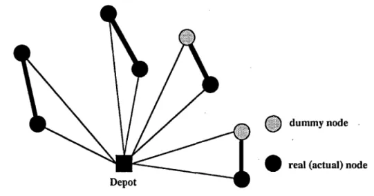
Using the aforementioned concepts, the solution with six customer nodes (Figure 2) is used to elaborate the idea of a parallel savings method for solu-tion: suppose T = 1 and the dummy number of points will be dnt = 4, then five tours will be generated; suppose T = 2 and the dummy number of points will be dni — 2, then four tours will be generated; suppose T = 3 and the dummy number of points will be dnt = 0, then three tours will be generated. Therefore, several trials of diverse loading combinations can be attempted, based on characteristics of the matching problem and the consideration of tour arrangements as a whole.
dummy node
^ P real (actual) node Depot
FIGURE 2 The Solution Concept for the Parallel Savings Method.
The symmetrical assignment problem and assignment problems (the core of VRPTW) differ mainly in that the symmetrical assignment problem can contrive every two points as one subtour. That subtour can be seen as a connected segment which enjoys the same significance as that of the matching problem (Burkard and Derigs, 1980). If the matching two points are regarded as one and are further iterated as a matching problem, it can be taken as a polynominal-time problem, and an approximate solution to TSP is found upon consideration of its comprehensiveness. Moreover, the solution to a symmetrical assignment problem, from the viewpoint of the cost matrix, will be in symmetry at those two cells. Those two cells respectively indicate the combined position and their end-points. The point of integration is an impor-tant index to record and transmit time window information.
In terms of the characteristics of the matching problem, the directionality incurred by the time window is actually the priority of customers, which happens to be a mutual contradiction. Of course, the data structure has to be adjusted so that the asymmetry characteristic of the problem is eliminated. From equation (4) the index representing "flexibility of scheduling" being
Fij = Min(/,- + Si + ttj, lj) — Max(e,- + s,- + ttj, ey) and the preliminary
assumptions of the discussed symmetry network by Euclidian space in this paper can be known. Through them we can conclude that the directionality is determined by "flexibility of scheduling". "Flexibility of scheduling" affects not only the duration of the waiting time, but also the length saved from the total routing distance. To speak in general terms, the greater the flexibility of
scheduling, the higher the probability that tours can be combined. The more the frequency of the combinations, the more distance can be saved from the total routing distance. Based upon the objective of the minimum total routing distance, a wider direction can be selected for "flexibility of scheduling" as its routing direction while the asymmetrical cost matrix can be transformed as being symmetrical.
To adjust to the flexibility of scheduling of tours, time windows (entry window, exit window or the original time windows of customers) are likely to change whenever there is any act of merging. As a result, should there be iteration, the starting and finishing points of the time window have to be revised. Such changes will impact on the spatial and temporal bi-criteria indices. With these adjustments, the effects can be fed back into the system after scheduling.
3.3. The Algorithm of the Spatial and Temporal Bi-criteria Parallel-savings-based Heuristic
The algorithm of the spatial and temporal bi-criteria parallel savings based heuristic is as follows:
STEP 0 Consider every customer as one tour and determine the number re-duced after every iteration, which will be the value of T.
STEP 1 Use equations (1) and (2) to find out the savings value and have it normalized.
STEP 2 Use equation (4) to cope with time-window and loading limit so as to find the flexible scheduling. If constraints are violated, flexibility of scheduling will be rendered negative to its unlimited greatness; use equation (3) again to have it normalized.
STEP 3 Use equation (5) to calculate the index value of the spatial and tem-poral bi-criteria.
STEP 4 Resolve the routing direction and transform the asymmetrical cost matrix to symmetry.
STEP 5 Insert the set of dummy nodes M,- and solve for the matching problem of the greatest weight; the number of these dummy nodes will be [Af,-| = (2xn-2x/xT-yM).
STEP 6 Modify the time window and loading amount, and examine the time window and loading limit so as to revise the index values of the spatial and temporal bi-criteria.
STEP 7 If limits are not yet fully violated, one additional iteration should be conducted and the process should proceed to step 2, otherwise to step 8. STEP 8 List the flexibility of every individual tour and calculate the vehicle starting time, total routing distance, total scheduling time and total waiting time of each tour at every depot.
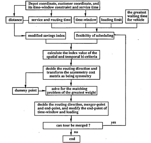
The relationships between and the operation of every variable can be seen in Figure 3. From the algorithm of the spatial and temporal bi-criteria parallel-savings method, it is found that when T = 1, only one point is reduced with every iteration, and the two tours with the greatest saving amount are merged with each iteration, resulting in a similar significance as that of the saving method contrived from conventional tours.
As can be seen from the solution flow chart and the assumption of a Euclidian spatial network, whether two tours can be merged is dependent
Depot coordinate, customer coordinate, and its time-window constraint and service time
distance — service and routing time time-window loading limit!
L
the greatest waiting time for vehicle
-»-] modified savings index flexibility of scheduling
X
calculate the index value of the spatial and temporal bi-criteria
\
dummy point
decide the routing direction and transform the asymmetry cost
matrix as being symmetry
solve for the matching problem of the greatest weight
decide the routing direction, merger-point and end-point, and modify the end-point of time-window and loading
can tour be merged ? yes
end
FIGURE 3 The solution flow chart of the spatial and temporal bi-criteria parallel-saving method.
on the limits of the time windows and loadings. If the flexibility of scheduling is decided on the one hand, the set of feasible solutions can be solved in the meantime. Suppose the time window to wait for any customer is started among any of the tours, flexibility of scheduling will be negative and the width of exit (entry) window will be zero, suggesting the punctuality to start the vehicle at this tour. In other words, either the waiting time of the vehicle will be increased or the limit of the time window ignored. Upon it, the peak time slot of outgoing goods is given, from the perspective of the internal operation of the depot. The information can also be referred to for the sorting order of picking-up goods at the depot. Furthermore, the designation of the greatest waiting time, for vehicles Max W, will affect the size of the feasible solution set, the total waiting time and the number of tours. In most of the cases, Max
W, within a specified range, reveals positive relationships with regard to the
size of the feasible solution set and the total waiting time, and vice versa to the number of tours.
4. TEST OF EXAMPLES
This section tests examples of the spatial and temporal bi-criteria parallel savings method presented in this paper. Since the tightness of the time windows is supposed to respond to the degree of difficulty of the problem, two sets of tightness are considered in this study. The magnitude of tightness £2 is indi-cated in equation (6); if £2 = 0, it is purely a scheduling problem; if £2 = 1, all time windows are equal (Desrocher, 1988).
x(MAX{/,}-MIN{e,}) (6) Thirty examples with fifty customer points in each example have been the subject of testing. These examples have been randomly created (0 < random < 1) and have utilized the traits of this randomness to design two sets of tightness for the time window. The illustration of Q < 0.5 is generated in such a manner to deliberately avoid over-concentration on the time window. The contents are: 1. Suppose that customers are spread throughout the rectangle of 90 x 90, the
coordinates (x, y) of the customers will be:
x = random x 90
y = random x 90 where 0 < x, y < 90. They will also be integers.
2. The depot will be positioned in the center of the rectangle 30 x 30, whose
coordinates (xx, yy) will be:
xx = 30 + random x 30 yy = 30 + random x 30
where 30 < xx, yy < 60. They will also be integers. 3. The amount q demanded by the customer:
q = 10 + random x (quantity of vehicle loading/12)
where 10 < q < 10 + (quantity of vehicle loading/12). It will also be an integer.
4. The starting point, width and service hour of the time window, which are: (1) the time window with a greater value of tightness:
e = 30 + random x 200 I = e + 10 + random x 110 s = 10 + random x 10
where (e, I) are the starting and finishing points of the time window, 30 <
e < 230, 40 < / < 350, 10 < time-window width < 120; s is the service
hour, 10 < s < 20.
(2) the time window with a smaller value of tightness:
e = 30 + random x 400
/ = e + 10 + random x 50
s = 10 + random x 10
where (e, Z) are the starting and finishing points of the time window, 30 <
e < 430, 40 < / < 490, 10 < time-window width < 60; s is the service hour,
10 < s < 20.
Performance comparisons are done by the insertion method of Baker and Schaffer (1986) (NSRTNB) and by that of Solomon (1987) (NSRTNS). The values of tightness of these two sets of test examples are shown in Table I.
The difference between NSRTNB and NSRTNS solutions is based on their different approaches and assumptions. The following is an elaboration of these criteria for generating better solutions of these insertion methods and their differences. Suppose i and j are two consecutive points on some known tour,
u is the insertion point; dy is the distance between i and j ; bi is the time that
point i is to be serviced; bj = MAX(ej,bj + si + f,;); bjU will be the time that point j is to be serviced after the insertion of point u, if e,-, /,-, Sj, f,;- are defined,
as in section 3. The increased distance will be en = dju + dUj — djj after the
TABLE I Characteristics of the Test Examples
Sets Values of Tightness
Wide Time Window Narrow Time Window
18.96-25.29% 7.09-9.15%
insertion of point u; the delay of service hour downstream is cyi = bju — by, the best criteria for better solutions proclaimed by Baker and Schaffer, and Solomon are respectively 2 x dou — en and 2 x dou — c\2. The former relies mainly on spatial criteria while the latter relies more on temporal criteria. The objective of BPSAD (the performance of the method studied in this paper) is based on minimising total routing distance. The objective of BPSAS (the performance of the method studied in this paper) is based on total scheduling time, and for BPSAW (the performance of the method studied in this paper) the objective is based on shortest waiting time.
The results of the first set of test examples, are as follows: given evaluation criteria as the number of tours, total routing distance and total scheduling time, the preciseness and stability of the solution derived from the spatial and temporal bi-criteria parallel-savings method is much higher than that of the insertion method, which is as indicated in Tables II and III.
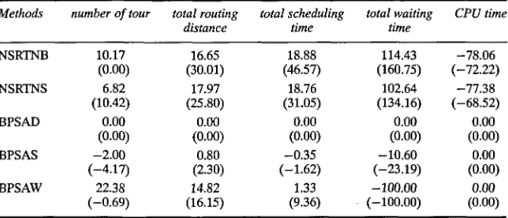
The results of the second set of test examples are as follows: given evalua-tion criteria as the number of tours, total routing distance, total scheduling time and total waiting time, the preciseness and stability of the solution derived from the spatial and temporal bi-criteria parallel-savings method is much higher than that of the insertion method, which is as indicated in Tables IV and V.
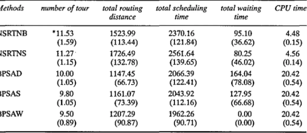
TABLE II The Average Performance of the First Set of Test Examples by the Insertion Method and the Bi-criteria Parallel-Savings Method
Methods NSRTNB NSRTNS BPSAD BPSAS BPSAW number of tour * 11.53 (1.59) 11.27 (1.15) 10.00 (1.05) 9.80 (1.05) 9.50 (0.89) total routing distance 1523.99 (113.44) 1726.49 (132.78) 1147.45 (66.73) 1161.07 (73.39) 1207.29 (90.87) total scheduling time 2370.16 (121.84) 2561.64 (139.65) 2066.39 (122.41) 2043.92 (112.16) 1962.26 (90.71) total waiting time 95.10 (36.62) 80.25 (46.02) 164.04 (78.08) 127.95 (66.68) 0.00 (0.00) CPU time 4.48 (0.15) 4.56 (0.14) 20.42 (0.54) 20.42 (0.54) 20.42 (0.54)
•denotes mean and (variance).
TABLE III The Comparative Performance (%) of the First Set of Test Examples by the Insertion Method and the Bi-criteria Parallel-Savings Method
Methods NSRTNB NSRTNS BPSAD BPSAS BPSAW number of tour 15.30 (50.00) 12.70 (8.49) 0.00 (0.00) - 2 . 0 0 (-0.94) - 5 . 0 0 (-16.04) total routing distance 32.82 (70.00) 50.46 (98.98) 0.00 (0.00) 1.19 (9.98) 5.22 (36.16) total scheduling time 14.70 (-0.47) 23.97 (14.08) 0.00 (0.00) - 1 . 0 9 (-8.37) -5.04 (-25.90) total waiting time -42.03 (-53.10) -51.08 (-41.06) 0.00 (0.00) -22.00 (-14.60) -100.00 (-100.00) CPU time -78.06 (-72.22) -77.67 (-74.07) 0.00 (0.00) 0.00 (0.00) 0.00 (0.00)
TABLE IV The Average Performance of the Second Set of Test Examples by the Insertion Method and the Bi-criteria Parallel-Savings Method
Methods NSRTNB NSRTNS BPSAD BPSAS BPSAW number of tour * 10.83 (1.44) 10.50 (1.59) 9.83 (1.44) 9.97 (1.38) 12.03 (1.43) total routing distance 1711.02 (149.46) 1730.50 (144.62) 1466.85 (114.96) 1478.57 (117.6) 1684.28 (133.53) total scheduling time 2858.93 (189.58) 2856.06 (169.50) 2404.85 (129.34) 2396.46 (127.24) 2436.76 (141.44) total waiting time 396.73 (142.68) 374.92 (128.13) 185.02 (54.72) 165.41 (42.03) 0.00 (0.00) CPU time 4.48 (0.16) 4.62 (0.17) 20.42 (0.54) 20.42 (0.54) 20.42 (0.54) 'denotes mean and (variance).
TABLE V The Comparative Performance (%) of the Second Set of Test Examples by the Insertion Method and the Bi-criteria Parallel-Savings Method
Methods NSRTNB NSRTNS BPSAD BPSAS BPSAW number of tour 10.17 (0.00) 6.82 (10.42) 0.00 (0.00) - 2 . 0 0 (-4.17) 22.38 (-0.69) total routing distance 16.65 (30.01) 17.97 (25.80) 0.00 (0.00) 0.80 (2.30) 14.82 (16.15) total scheduling time 18.88 (46.57) 18.76 (31.05) 0.00 (0.00) - 0 . 3 5 (-1.62) 1.33 (9.36) total waiting time 114.43 (160.75) 102.64 (134.16) 0.00 (0.00) -10.60 (-23.19) -100.00 (-100.00) CPU time -78.06 (-72.22) -77.38 (-68.52) 0.00 (0.00) 0.00 (0.00) 0.00 (0.00)
Among these criteria, the insertion method shown as total waiting time does not perform as well as our method with the narrow time window. It indicates that this spatial and temporal bi-criteria parallel-savings method can solve scheduling problems.
From these two sets of test examples, the research method studied in this paper, based on the number of tours, total routing distance and total scheduling time, fares much better than does the insertion method. As for total waiting time, though it sometimes performs worse than the insertion method, this study can somehow control the duration of the waiting time and be considered as an external variant determined by the depot. Only if Max W = 0 would there be such toil caused by the increased number of tours. It has evidently shown itself in the second set of test examples. As for the balance between total waiting time and the number of tours, the depot is authorized to make its own decisions according to the policy of the depot.
5. CONCLUSION
There are a number of conclusions which can be drawn from this study. The research method devised in this study has been developed with a view to solving the three interdependent problems of routing, scheduling and loading from the vehicle routing problem with time windows (VRPTW). With regard to the routing problem, the revised savings index by Yellow is adopted; as for scheduling, "flexibility of scheduling" is recommended in this study as the index; in terms of the loading problem, the techniques of adding dummy points by Altinkemer and Gavish are modified. Thus, when solutions are to be generated for these three major keys, they will not be strait-jacketed into any particular category.
The spatial and temporal bi-criteria parallel-savings method is capable of manipulating the set of feasible solutions because of its management of tem-poral criteria. We can see that throughout the stages of tour contrivance, both the changes of time windows and loading are specifically recorded. Conse-quently, the matching problem is so adapted that the outcome as a whole is well administered.
In view of the test performance, the results of the comparison between this study and the insertion method indicate that the insertion method excels by 6% to 40% over that of the spatial and temporal bi-criteria savings method with regard to the number of tours, total routing distance and total scheduling time. No evident trend of superiority or inferiority (better or worse) is seen in the category of total waiting time; moreover, the duration length of the total waiting time is well under the direction of this study.
However, suppose the finishing point of the customer time window is smaller than the period the vehicle needs to run from the depot to the customer point. The insertion method will not be able to put this customer point into any point of the tour. Practically speaking, the insertion method cannot meet all customer needs in that no vehicle can set off earlier than scheduled to accom-modate the customer time window. The tour contrivance employed in this study was by "routing and scheduling dual disposition"; therefore, not only the above-mentioned problems can be taken care of, but also the interval between vehicles starting from the depot can also be delayed as scheduled, because of the flexibility of tours resulting from the width of entry (exit) window of tours "flexibility of scheduling". With such practices, the depot can manage the prior operations of goods delivery, such as sorting and arrangements of staff shifts.
The spatial and temporal bi-criteria savings method proposed here is the measure to manage the three major problems and to introduce certain adjust-ments so that routing, scheduling and loading problems can be resolved respec-tively. When h = 1, where h is the weighting of the index of spatial routing, the outcome will be the practice of a parallel savings method to resolve the vehicle routing problem; when h = 0 the outcome will be the method to resolve the scheduling problem; when the smallest difference between the total capacity and total loading is considered as the objective, it will then be the method to resolve the loading problem.
Reference
Altinkemer, K. and Gavish, B. L. (1991) "Parallel Savings based Heuristics for The Delivery Problem", Operations Research. 39, 456-469.
Baker, E. K. and Schaffer, J. R. (1986) "Solution Improvement Heuristics for the Vehicle Routing and Scheduling Problem with Time Window Constraints", American Journal of
Mathemat-ical and Management Sciences, 6, 261-300.
Burkard, R. E. and Derigs, U. (1980) "Assignment and Matching Problems: Solution Methods with FORTRAN-Programs", Lecture Notes in Economics and Mathematical Systems, Sprin-ger Verlag, No. 184.
Clarke, G. and Eright, J. W. (1964) "Scheduling Vehicles from a Central Delivery Depot to a Number of Delivery Points", Operational Research Quarterly, 12, 568-581.
Desrochers, M., Lenstra, J. K., Savelsbergh, M. W. P. and Soumis, F. (1988) "Vehicle Routing with Time Windows: Optimization and Approximation", Vehicle Routing: Methods and
Studies, B. L. Golden and A. A. Assad (Editors), Elsevier Science Publishers B.V., 65-84.
Golden, B. (1976) "Shortest Path Algorithms: a Comparison", Operations Research, 24, 1164-1168.
Golden, B. (1977) "Evaluating a Sequential Vehicle Routing Algorithm", AIIE Transactions, 9. 204-208.
Golden, B. and Assad, A. A. (1986) "Vehicle Routing with Time Window Constraints", American
Journal of Mathematical and Management Science, 6, 251-260.
Kolen, A., Rinnooy Kan, A. and Trienkekens, H. (1987) "Vehicle Routing with Time Windows",
Operations Research, 35, 266-273.
Koskosidis, Y., Powell, W. and Solomon, M. (1992) "An Optimization Based Heuristic for Vehicle Routing and Scheduling with Soft Time Window Constraints", Transportation
Science, 26, 69-85.
Mole, R. H. and Janeson, S. R. (1976) "A Sequential Route-builting Algorithm Employing Gene-ralized Savings Criterion", Operational Research Quarterly, 27, 503-511.
Solomon, M. M. (1986) "On the Worst-case Performance of Some Heuristics for the Vehicle Routing and Scheduling Problem with Time Window Constraints", Networks, 16, 161-174. Solomon, M. M. (1987) "Algorithms for the Vehicle Routing and Scheduling Problems with
Time Window Constraints", Operations Research, 35, 254-265.
Teodorovic, D., Kikuchi, S. and Hohlacov, D. (1991) "A Routing and Scheduling Method in Considering Trade-off Between the User's and the Operator's Objectives", Transportation
Planning and Technology, 16, 63-75.
Van Landeghem, H. R. G. V. (1988) "A Bi-criteria Heuristic for the Vehicle Routing Problem with Time Windows", European Journal of Operational Research, 36, 217-226.
Yellow, P. C. (1970) "A Computational Modification to the Savings Method of Vehicle Schedu-ling", Operational Research Quarterly, 21, 281-283.