International Research Journal of Finance and Economics ISSN 1450-2887 Issue 27 (2009)
© EuroJournals Publishing, Inc. 2009 http://www.eurojournals.com/finance.htm
Forecasting Efficiency of Implied Volatility and the Intraday High-Low Price Range in Taiwan Stock Market
Chih-Hsing Hung
Department of Finance, Fortune Institute of Technology Kaohsiung County, Taiwan, R.O.C
E-mail: [email protected] Shyh-Weir Tzang
Department of Finance, Yung Ta Institute of Technology Ping-Tong County, Taiwan, R.O.C
E-mail: [email protected] David So-De Hsyu
Department of Finance, National Sun-Yat Sen University Kaohsiung, Taiwan, R.O.C
E-mail: [email protected] Abstract
The paper compares the efficacy of high low range volatility and implied volatility indexes in volatility forecasting. VIX and VXO, the constructed volatility indexes of Taiwan stock market, are usually believed to deliver effective forecasts of stock index return volatility. Based on the econometric models examined in the paper, the high low range volatility is found to provide volatility forecasting at least as efficient as do the volatility indexes. For smaller in-sample size, however, VIX is more efficient than other models in volatility forecast. In a market like Taiwan where volatility index may be hard to measure with accuracy due to a less liquid option trading, the high low range volatility, in combination with VIX, can be used by practitioners as alternative tools in investment decisions and risk management.
Keywords: VIX, VXO, GJR GARCH, volatility forecasting, JEL Classification Codes: C13, C22, C53, G14
1. Introduction
VXO and VIX are well-known indexes which are widely used to measure the perception of the option traders on stock market forward volatility. The VXO which CBOE has computed since 1993, originally called VIX, is the implied volatility of a hypothetical 30-calendar-day at-the-money S&P 100 index option. CBOE further introduced a new VIX volatility index in 2003 without using any particular option-pricing model. The new VIX incorporates information from the volatility skew by using a wider range of option series than just at-the-money option series. The so-called model-free implied volatilities provide ex-ante risk neutral expectations of the future volatilities (Dupire, 1993; Carr and
Madan, 1998; Britten-Jones and Neuberger, 2000; Lynch and Panigirtzoglou, 2003; Carr and Wu, 2005).
Whaley (2000) has indicated that many investors will agree with the fact that when stock prices get higher, investors will raise their concern on stock prices. The level of concern which reflects the investors’ consensus view or sentiment on stock prices or market index can be represented by the forward volatility implied by traded options. Implied volatility has been gaining attention from institutions and academics for its ability in predicting future market volatility.
For researchers and investors, the information content and forecast quality of implied volatility has become an important subject of research in recent years. Harvey and Whaley (1991) find that the implied volatility is able to forecast the forward volatility of the market. The forecast quality of implied volatility has been widely reviewed by a large amount of literature such as Latane and Rendleman (1976), Chiras and Manaster (1978), and Beckers (1981). They find that the implied volatility provides better estimates of future return volatility than standard deviations obtained from historical returns.
Jorion (1995) also finds that the implied volatilities from options on foreign exchange offer better estimates than do the historical prices
Different results are also found by Day and Lewis (1988), Lamoureux and Lastrapes (1993) and Canina and Figlewski (1993). Their empirical studies show that the implied volatility is not qualified as a good predictor for future return volatilities. Christensen and Prabhala (1998) refuted their results by showing that the weakness of the implied volatility in future volatility prediction is mainly resulted from the methodological issues like overlapping sample and mismatched maturities.
Blair, Poon, and Taylor (2001) further find that implied volatilities from option prices of S&P 100 index deliver better volatility forecasts than those obtained from either low- or high-frequency index returns. Corrado and Miller (2005) examine the forecast quality of three implied volatility indexes based on S&P100 (VXO), S&P500 (VIX) and Nasdaq 100 (VXN). Their empirical results reveal that the forecast quality of VXO and VIX has been improved since 1995 and VXN even provides better quality forecasts of future volatility.
The academic analysis of price range, which is defined as the difference between the highest and lowest prices of assets over some time interval, can be dated back to Parkinson (1980) and Garman and Klass (1980) and has seen a rapidly expanding literature on range-based volatility in recent years.
The empirical results show that variances measured by range estimators efficiently approximate the daily integrated variance. The performance evaluation of range-based estimators in literature can be found in Shu and Zhang (2006). Survey references include Poon (2005), McAleer and Medeiros (2008) and Chou et al. (2008).
Corrado and Truong (2007) finds that the intraday high-low price range provides volatility forecast as efficient as high-quality implied volatility indexes published by CBOE on four stock indexes. The advantages of high-low price range as a volatility forecast motivates us to conduct relevant regression analyses to compare the forecast efficiency of price range with volatility indexes.
The paper is structured as follows: section 2 is the data and methodology; section 3 is the empirical results; section 4 provides the concluding remarks.
2. Data
The sample period spans from 2004/1/2 to 2007/12/31 with a total trading days of 992. The options data before 2004 are excluded as the trading of options is still thin in comparison with the trading in subsequent years. The intraday prices of index options (with ticker symbol TXO) are obtained from Taiwan Futures Exchange (TAIFEX). Taiwan stock market index (TAIEX) is obtained from Taiwan Economic Journal (TEJ). Four kinds of data to be examined are described as below: VXO, VIX, daily squared returns and high low range volatility.
194 International Research Journal of Finance and Economics - Issue 27 (2009) 2.1. Volatility Indexes
By the white paper published by CBOE, VXO is constructed by using the implied volatilities of eight nearby and second-nearby options series with the nearest at-the-money strikes. The eight option series are equally divided into two groups: nearby and second-nearby options. For the nearest at-the-money options, there are two pairs of call/put option series with strike prices just bracketing the underlying stock index respectively. To compute the VXO, the term structure of volatility is assumed to be linear, and the implied volatility with 22 trading days (30 calendar days) to expire can be interpolated. Let
t1
N and N be the days to expiry for nearby and second nearby options. VXO will be obtained as follows: t2
2 1
2 1 2 1
1 2
22 22
VXO t t
t t t t
N N
N N N N
σ ⎛ − ⎞ σ ⎛ − ⎞
= ⎜⎜⎝ − ⎟⎟⎠+ ⎜⎜⎝ − ⎟⎟⎠ (1)
where σ1 and σ2 are implied volatilities of the nearby and second nearby options, respectively.
The computation of VIX by CBOE is described in the following formula, in which C K T ( , ) and P K T denote prices of call and put options with strike price K and days to maturity T. By ( , ) assuming strike prices to be order such that Kj+1 >Kj, the restriction is further imposed on two maturities such that T2 ≥22≥ ≥ . T1 8
2
1 1
2
1 2 1 1
VIX ( 1) 22 min( ( , ), ( , ))
N
j j
h h
j h j h
h j j
K K
T C K T P K T
T T K
+ −
= =
− −
= −
∑
−∑
(2)To reduce biases in computing the volatility indexes, CBOE uses the prices of second nearby options to replace nearby options with 8 days to expire.
For options trading in Taiwan market, the second-nearby options and the next to second-nearby options have rather thin trading. To mitigate the biases from the unavailability of option prices required in computing VXO and VIX, the paper uses the average of all the mids of bid and ask prices for all options trading within the trading interval. The trading interval is set up to be 1-minute to compute intraday volatility series. Therefore, the daily closing VXO and VIX can be obtained for further analysis by the paper.
2.2. Daily Squared Returns and Range Volatility
One simple measure of realized volatility is adopted by the paper for comparison purpose: the squared daily returns which are computed from natural logarithms of closing levels of Taiwan Stock Exchange Index as a benchmark for forecasting:
2 2
1
Re tt ln ( t )
t
c c−
= (3)
Rett represents the index return for day t based on index levels at the close of c and t ct−1. The range-based volatility is computed by the formula suggested by Parkinson (1980):
2
2 ln ( / )
4 ln 2
t t
t
W = h l (4)
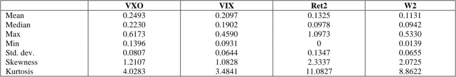
W represents the intraday high-low range volatility on day t. t h and t l denote the highest and lowest t price levels observed during trading on day t. To be consistent with other daily volatility measures, all implied volatility indexes are squared and divided by 252, the assumed number of trading days in a calendar year. The summary statistics of four measures and their correlation are reported in Table 1 and 2.
Table 1: Summary Statistics for Volatility Series (2004/1/2-2007/12/31) a
VXO VIX Ret2 W2
Mean 0.2493 0.2097 0.1325 0.1131 Median 0.2230 0.1902 0.0978 0.0942
Max 0.6173 0.4590 1.0973 0.5330
Min 0.1396 0.0931 0 0.0139
Std. dev. 0.0807 0.0644 0.1347 0.0655
Skewness 1.2107 1.0828 2.3337 2.0725 Kurtosis 4.0283 3.4841 11.0827 8.8622 a. Ret2 and W2 are the annualized volatility series based on daily squared returns and high-low price range.
Table 2: Correlations of the Volatility Series
VXO VIX Ret2 W2
VXO 1
VIX 0.9775 1
Ret2 0.4163 0.3973 1
W2 0.5845 0.5535 0.5714 1
3. Forecasting 3.1. Models
The paper uses the generalized autoregressive heteroskedasticity model, or GJR-GARCH model developed by Glosten, Jagannathan, and Runkle (1993), to account for the effect of good news and bad news on conditional volatility. The implied volatility indexes and high-low range volatility are included in the model for further examination. The augmented GJR-GARCH model is denoted as the following:
2 2 2 2
0 1 1 2 1 1 1 IVOL 1 1
t t
t t t t t t t
R
h s h W
μ ε
α α ε− α −ε− β − γ − δ −
= +
= + + + + + (5)
where R : return on day t; t h : conditional volatility on day t; t IVOLt−1: implied volatility at the end of option trading on day t-1; st−1: 1 if εt−1< , and 0 otherwise; 0 Wt−1: intraday high-low range volatility on day t-1. s is an indicator function to account for effect of the good news (t εt > )and bad news 0 (εt < ) on conditional variance. Therefore, the effect of good news is measured by 0 α1, and the effect of bad news is measured by (α α1+ 2). The effects of implied volatility and high-low range volatility on conditional variance are measured by coefficients γ and δ .
To assess the incremental information provided by implied volatilities and high-low price range, four models are examined as follows:
• Model 1: ht =
α
0+α ε
1 t2−1+α
2st−1ε
t2−1+β
ht−1• Model 2: ht =α α ε0+ 1 t2−1+α2st−1εt2−1+βht−1+γ IVOL2t−1
• Model 3: ht =α α ε0+ 1 t2−1+α2st−1εt2−1+βht−1+δWt2−1
• Model 4: ht =α α ε0+ 1 t2−1+α2st−1εt2−1+βht−1+γ IVOL2t−1+δWt2−1
In model 2 and model 4, the IVOL can be substituted for by VIX or VXO to evaluate their forecasting quality. Model 2-1 and 4-1 denote the IVOL replaced by VIX, and Model 2-2 and 4-2
196 International Research Journal of Finance and Economics - Issue 27 (2009) denote the IVOL replaced by VXO. To decrease the potential bias from large sample sizes leading to Type II errors, the critical test statistic values of t and F are also adjusted 1.
3.2. Out-of-Sample Forecasts and Efficiency Evaluations
As the sample size is limited to 992 days, the first 500-day data are used as in-sample data to estimate the required parameters. To ensure the stability of the estimated parameters, 250-day in-sample data are also used to estimate the parameters for comparison purpose. Based on the initial estimated parameters, the out-of-sample volatility forecasts are obtained for the next N=1, 10, 20 days after the estimation period. One day forecast is generated from each model specification. 10- and 20-day forecasts are obtained by multiplying 1-day volatility forecast by 10 and 20, respectively. The corresponding realized volatilities are computed as the sum of squared daily returns over each forecast period. The parameters are recalibrated by moving the sample window based on 250- and 500-day in- sample data. Four evaluation criteria are listed in the following:
• P-statistic: Suggested by Blair et al. (2001), P-statistic measures the proportion of the variances of realized volatilities explained by volatility forecasts.
( )/
2
( 1), ( 1),
1 ( )/
2 ( 1), 1
ˆ
( )
1
( )
T S N
S N i N S N i N
i
T S N
S N i N
i
y y
P
y y
−
+ − + −
=
−
+ −
=
−
= −
−
∑
∑
(6),
yt N denotes realized volatility measured as the sum of squared daily returns over an N-day forecast period beginning on day t, and yˆt N, denotes the corresponding volatility forecast for the same forecast period. For the data of TAIEX used in the paper, T=992 and S=250 and 500 for the two sample periods.
N is the forecast horizon of 1, 10 and 20 days.
• Root mean square error (RMSE):
( )/ 2
( 1), ( 1),
1
1 ˆ
RMSE ( ) / T S N
(
S N i N S N i N)
i
y y
T S N
−
+ − + −
=
= −
−
∑
(7)• Mean absolute error (MAE):
( )/
( 1), ( 1),
1
1 ˆ
MAE | |
( ) /
T S N
S N i N S N i N
i
y y
T S N
−
+ − + −
=
= −
−
∑
(8)• R from the following regression: 2
, ˆ,
t N t N t
y = +α β y + (9) e
R measures the ability of volatility forecast 2 yˆt N, to explain the corresponding N-day realized volatility yt N, .
By following Blair et al. (2001) to compare forecasts from Models 2-1, 2-2 and 3, the forecast errors from each model are regressed on forecasts from model 2 and 3 specified in the following:
3
2 2
, ˆM, 1 2 ˆM, 3 ˆM,
t N t N t N t N t
y −y = +a a y +a y +ε (10)
3 2 3
, ˆM, 1 2 ˆM, 3 ˆM,
t N t N t N t N t
y −y = +b b y +b y +ε (11)
2
ˆt NM,
y and yˆt NM,3 denotes an N-day forecast from model 2 and model 3, respectively. The forecasts
2
ˆt NM,
y and yˆt NM,3 are regarded as efficient when R values from the above two regressions are not 2
1 As shown by Lindley's paradox, the t-and F-statistics are adjusted when their absolute values are greater than the value of the following: * 1/ * 1 ( 1)/
( 1), ( 1)
1
T T k T
t T k T F T
K
− −
= − × − = × −
− where T is the sample size and k is the number of degrees of freedom lost in the regression.
significantly different from zero. The null hypothesis of a1 =a2 = (or 0 b1 =b2 = ) is also tested to see 0 if there is any forecasting errors left unexplained by the model examined.
4. Empirical Results
4.1. Estimation of Models by In-Sample Data
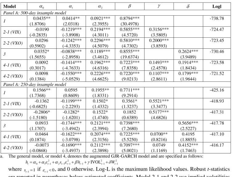
Table 3 shows the results of GJR-GARCH estimated parameters and related statistics across all models and different sample sizes. To account for effects of different sample sizes on estimated parameters, the results of the estimated parameters by 250-day sample size are reported in panel B. Model 2-1 and 2-2 denote the variable IVOL which is substituted for by VIX and VXO respectively. Similar notation applies to model 4. Columns 2 through 7 state estimated parameter values with robust t-statistics in parentheses.
Table 3: Summary of GJR-GARCH Estimated Parameters Based on 500- and 250-in-Sample Data a
Model α0 α 1 α 2 β γ δ Logl
Panel A: 500-day insample model
0.0435** 0.0414** 0.0921*** 0.8794*** -738.78 1 (1.8706) (2.0318) (2.3955) (30.4978)
-0.0190 -0.1219*** 0.2194*** 0.5855*** 0.3156*** -724.47 2-1 (VIX)
(-0.2835) (-3.8908) (4.3011) (4.5720) (3.5805)
0.0296 -0.1242*** 0.2296*** 0.5810*** 0.2000*** -723.45 2-2 (VXO)
(0.5902) (-4.3353) (4.5079) (4.7302) (3.8593)
0.0352* -0.0838*** 0.1189*** 0.8555*** 0.2624*** -730.46 3 (1.5655) (-2.8958) (3.4612) (19.6374) (3.9489)
0.0092 -0.1414*** 0.1962*** 0.7223*** 0.1493*** 0.1914*** -723.58 4-1 (VIX)
(0.3017) (-4.7633) (4.6316) (7.8358) (2.4578) (1.8434)
0.0098 -0.1550*** 0.2226*** 0.7220*** 0.1107*** 0.1799*** -721.52 4-2 (VXO)
(0.1384) (-5.0529) (4.6625) (9.0213) (2.8611) (1.9644) Panel A: 250-day insample model
0.1566** 0.0595 0.1955** 0.7711*** -425.16 1 (1.7368) (0.8609) (1.8331) (9.2914)
-0.1362 -0.1199*** 0.1502* 0.3561* 0.5521*** -418.93 2-1 (VIX)
(-0.6825) (-2.2293) (1.4332) (1.3237) (3.3477)
-0.2806* -0.1282* 0.1522* 0.1852 0.5177*** -417.31 2-2 (VXO)
(-1.5180) (-1.6201) (1.4740) (0.6389) (4.6826)
0.0933 -0.1744*** 0.2121*** 0.7398*** 0.5656*** -417.78 3 (1.1707) (-3.4942) (2.3994) (7.2680) (2.5227)
0.0464 -0.1622*** 0.2074*** 0.7225*** 0.0700** 0.4195 -417.10 4-1 (VIX)
(0.1874) (-3.0798) (2.3156) (5.5250) (0.8216) (1.8855)
-0.0073 -0.1690*** 0.2112*** 0.7097*** 0.0749 0.4152*** -416.17 4-2 (VXO)
(-0.0868) (-3.4937) (2.3898) (5.0021) (1.1169) (1.7463) a. The general model, or model 4, denotes the augmented GJR-GARCH model and are specified as follows:
2 2 2 2
0 1 1 2 1 1 1 IVOL 1 1
t t t t t t t
h =α α ε+ − +α s−ε− +βh− +γ − +δW−
where st−1=1 if εt−1<0, and 0 otherwise. Log-L is the maximum likelihood values. Robust t-statistics are reported in parentheses below estimated coefficients. Model 2-1 and 2-2 use implied volatilities based on VIX and VXO, respectively. The same notation applies to model 4.
b. The notations of *, ** and *** represent 0.1, 0.05 and 0.01 significance level, respectively.
In panel A, Model 4-2 yields the largest log-likelihood value, followed by Model 2-2 and 4-1.
The estimated parameters in Model 4-2 are all significantly different from zero except the constant term. When sample size decreases to 250, Model 4-2 in panel B still has the largest log-likelihood value, followed by Model 4-1 and 2-2. However, the estimated parameter γ in Model 4-2 becomes
198 International Research Journal of Finance and Economics - Issue 27 (2009) insignificant, suggesting that the explanatory power of VXO may not be stable with variant sample sizes.
In panel A and B, α1is negative and significantly different from zero for Model 2, 3 and 4. α2, which measures the effect of good news, is positive and significant for all models in both panels.
Moreover, (α α1+ 2)for models 2, 3 and 4 are all positive, indicating the existence of asymmetric news effect which is consistent with Corrado and Truong (2007).
γ and δ are significant for all models in panel A. However, γ is insignificant in Model 4-1 and 4-2 of panel B. In the general Model 4-1 and 4-2, the forecasting ability of volatility index tends to increases with in-sample size, but the absolute values of γ are smaller than those of δ , suggesting that the intraday high-low range volatility dominates implied volatility index in predicting the conditional volatility 2.
4.2. Out-of-Sample Forecast Evaluation
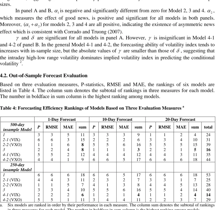
Based on three evaluation measures, P-statistics, RMSE and MAE, the rankings of six models are listed in Table 4. The column sum denotes the subtotal of rankings in three measures for each model.
The number in boldface in sum column is the highest ranking among models.
Table 4: Forecasting Efficiency Rankings of Models Based on Three Evaluation Measures a
1-Day Forecast 10-Day Forecast 20-Day Forecast 500-day
insample Model P RMSE MAE sum P RMSE MAE sum P RMSE MAE sum total
1 3 3 5 11 3 3 3 9 1 1 2 4 24
2-1 (VIX) 6 6 3 15 2 2 2 6 3 3 4 10 31
2-2 (VXO) 1 1 6 8 5 5 6 16 5 5 5 15 39
3 2 2 4 8 1 1 1 3 2 2 1 5 16
4-1 (VIX) 5 5 2 12 4 4 4 12 4 4 3 11 35
4-2 (VXO) 4 4 1 9 6 6 5 17 6 6 6 18 44
250-day insample Model
1 6 6 6 18 6 6 5 17 6 6 6 18 53
2-1 (VIX) 4 4 3 11 2 3 2 7 3 3 1 7 25
2-2 (VXO) 1 1 5 7 4 1 3 8 4 4 5 13 28
3 3 3 4 10 5 5 6 16 5 5 4 14 40
4-1 (VIX) 2 2 2 6 1 2 1 4 1 1 2 4 14
4-2 (VXO) 5 5 1 11 3 4 4 11 2 2 3 7 29
a. Six models are ranked in order by their performance in each measure. The column sum denotes the subtotal of rankings in three measures for each model. The number in boldface in sum column is the highest ranking among models.
For the 500-day in-sample data in Table 4, Model 3 ranks highest among all models, indicating that volatility index is less effective in volatility prediction than expected. For 1- and 10-day forecast in panel A, Model 3 ranked highest. For 20-day forecast, model 1and 3 ranked first and second. For 250- day in-sample data, Model 4-1 ranked highest in terms of overall rankings. Model 4-1 also ranked highest for 1-, 10- and 20-day forecasting periods. When the in-sample size increases from 250 to 500 days, the high-low range volatility seems to subsume VIX as a dominating factor in volatility prediction. The result is also consistent with the Corrado and Truong (2007) that the high low range volatility is no less efficient than VIX in volatility prediction.
2 The paper also used 125-day in-sample data to estimate γ and δ in Model 4. Both estimated coefficients are not significantly different from zero.
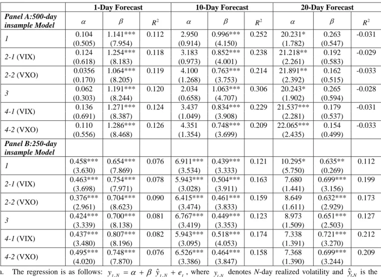
Table 5: Regression of Realized Volatility Against Out-of-Sample Volatility Forecasts a
1-Day Forecast 10-Day Forecast 20-Day Forecast Panel A:500-day
insample Model α β R2 α β R2 α β R2
0.104 1.141*** 0.112 2.950 0.996*** 0.252 20.231* 0.263 -0.031 1 (0.505) (7.954) (0.914) (4.150) (1.782) (0.547) 0.124 1.254*** 0.118 3.183 0.852*** 0.238 21.218** 0.192 -0.029 2-1 (VIX)
(0.618) (8.183) (0.973) (4.001) (2.261) (0.583) 0.0356 1.064*** 0.119 4.100 0.763*** 0.214 21.891** 0.162 -0.033 2-2 (VXO)
(0.170) (8.205) (1.268) (3.753) (2.392) (0.515) 0.062 1.191*** 0.120 2.034 1.063*** 0.306 20.243* 0.265 -0.028 3 (0.303) (8.244) (0.658) (4.707) (1.902) (0.594) 0.136 1.271*** 0.124 3.437 0.834*** 0.229 21.537*** 0.179 -0.031 4-1 (VIX)
(0.691) (8.387) (1.049) (3.908) (2.281) (0.537) 0.110 1.286*** 0.126 4.351 0.748*** 0.209 22.065*** 0.154 -0.033 4-2 (VXO)
(0.556) (8.468) (1.354) (3.699) (2.435) (0.499) Panel B:250-day
insample Model
0.458*** 0.654*** 0.076 6.911*** 0.439*** 0.121 10.295* 0.635** 0.112 1 (3.630) (7.869) (3.534) (3.333) (5.750) (0.269)
0.463*** 0.754*** 0.078 5.943*** 0.504*** 0.163 7.680 0.699*** 0.199 2-1 (VIX)
(3.698) (7.971) (3.028) (3.911) (1.441) (3.156) 0.376*** 0.704*** 0.090 6.415*** 0.461*** 0.159 8.649 0.632*** 0.173 2-2 (VXO)
(2.961) (8.623) (3.474) (3.833) (1.611) (2.929) 0.424*** 0.700*** 0.081 6.767*** 0.449*** 0.123 8.973 0.651*** 0.127 3 (3.339) (8.138) (3.419) (3.353) (1.509) (2.503)
0.437*** 0.807*** 0.082 5.943*** 0.518*** 0.174 7.338 0.721*** 0.212 4-1 (VIX)
(3.480) (8.196) (3.095) (4.053) (1.391) (3.270) 0.495*** 0.748*** 0.076 6.526*** 0.464*** 0.158 7.368 0.699*** 0.209 4-2 (VXO)
(4.020) (7.870) (3.386) (3.847) (1.390) (3.244) a. The regression is as follows: yt N, =α + β yˆt N, +et , where yt N, denotes N-day realized volatility and yˆt N, is the
volatility forecast for the same period. Robust t-statistics are reported in parentheses below estimated coefficients.
Table 5 reported the estimated coefficients and R2 values from regressing the realized volatility on out-of-sample volatility forecasts across models and periods based on two in-sample sizes. For 500- insample data, Model 3 has the highest R2 of 0.306 for 10-day forecast. For 1-day forecast, Model 4-1 and 4-2 have higher R2 values of 0.124 and 0.126 than other models. However, their efficacy decreases as forecast period increases to 10 and 20 days. For 20-day forecast, all models have insignificant R . 2
For 250-insample data in panel B, Model 4-1 consistently delivered better results (the highest R ) than other models. In general, for 500-day in-sample data, Model 4-1 and 4-2 yielded better 2
results for 1-day forecast; Model 3 is better in 10-day forecast and has the highest R value among all 2 models. For 250-day in-sample data, Model 4-1 consistently performs better than others across all forecast periods.
Based on the seemingly mixed results in the above, however, a more consistent conclusion can be made that VIX is more dominant than VXO in predicting future volatility. But the effectiveness of forecasting by VIX is not evident in the framework of a large sample size.
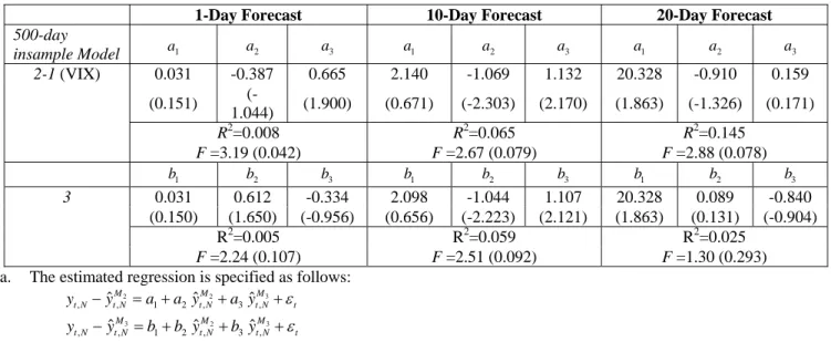
200 International Research Journal of Finance and Economics - Issue 27 (2009) Table 6: Regression of Volatility Forecast Errors on Forecasted Values by Model 2-1 and Model 3 a
1-Day Forecast 10-Day Forecast 20-Day Forecast 500-day
insample Model a1 a2 a3 a1 a2 a3 a1 a2 a3
0.031 -0.387 0.665 2.140 -1.069 1.132 20.328 -0.910 0.159 (0.151) (-
1.044) (1.900) (0.671) (-2.303) (2.170) (1.863) (-1.326) (0.171) R2=0.008 R2=0.065 R2=0.145
2-1 (VIX)
F =3.19 (0.042) F =2.67 (0.079) F =2.88 (0.078)
b1 b2 b3 b1 b2 b3 b1 b2 b3
0.031 0.612 -0.334 2.098 -1.044 1.107 20.328 0.089 -0.840 (0.150) (1.650) (-0.956) (0.656) (-2.223) (2.121) (1.863) (0.131) (-0.904)
R2=0.005 R2=0.059 R2=0.025 3
F =2.24 (0.107) F =2.51 (0.092) F =1.30 (0.293)
a. The estimated regression is specified as follows:
3
2 2
, ˆM, 1 2 ˆM, 3 ˆM,
t N t N t N t N t
y −y = +a a y +a y +ε
3 2 3
, ˆM, 1 2 ˆM, 3 ˆM,
t N t N t N t N t
y −y = +b b y +b y +ε
2
ˆt NM,
y denotes an N-day forecast from Model 2-1. The results of forecast errors in Model 3 are obtained from the second equation. The parentheses below each estimated coefficient are t-statistics. F-statistics and their corresponding p-value in the parentheses are also listed.
Table 6 reports the regression results by regressing the volatility forecast errors on the out-of- sample forecasted values by Model 2-1 and Model 3, respectively. If the forecasts made by Model 2-1 or Model 3 are efficient, the coefficients a and 1 a , or 2 b and 1 b , are expected be insignificantly 2 different from zero. The value of F-test on the null hypothesis of a1=a2 = (or 0 b1=b2 = ) is 0 reported with its corresponding P value. For the 500-day in-sample data, all R2 values are not significantly different from zero at critical p level of 0.01. For 250-day in-sample data in Table 7, Model 2-1 and Model 3 delivered efficient forecasts only for 20-day forecast period (with 5%
significance level for F test). In general, the forecasting efficiency of Model 2-1 and Model 3 is found to be more efficient in forecasting as the sample size increases from 250 to 500.
Table 7: Regression of Volatility Forecast Errors on Forecasted Values by Model 2-1 and 3
1-Day Forecast 10-Day Forecast 20-Day Forecast 250-day insample
Model a1 a2 a3 a1 a2 a3 a1 a2 a3
0.403 -0.668 0.429 6.019 -0.055 -0.466 9.383 0.165 -0.565 (0.127) (0.213) (0.194) (3.067) (-0.125) (-1.045) (1.640) (0.277) (-0.841)
R2=0.013 R2=0.159 R2=0.145 2-1 (VIX)
F =5.84 (0) F =7.91 (0) F =1.26 (0.295)
b1 b2 b3 b1 b2 b3 b1 b2 b3
0.403 0.331 -0.570 6.019 0.944 -1.466 9.383 1.165 -1.565 (0.127) (0.213) (0.194) (3.067) (-0.125) (-1.045) (1.640) (1.952) (-2.330)
R2=0.016 R2=0.218 R2=0.094 3
F =7.28 (0) F =11.17 (0) F =2.87 (0.070)
5. Conclusion
The volatility index has been widely accepted as an indicator to measure the sentiments of investors. In emerging market like Taiwan, however, the volatility index is still new to many investors. According to CBOE, the nearby and second nearby options prices will be used in the construction of the volatility series. However, the illiquid trading of the second nearby options in Taiwan may create missing data in computing the volatility index.
To gain more insight into the options market in Taiwan, the paper tries to construct the volatility indexes by different sampling methods to obtain a better measure of implied volatility series.
The paper uses the average of all the mids of bid and ask prices on options to reconstruct the volatility index series, in the hope of delivering more accurate measures of the volatility indexes like VIX and VXO.
The paper further compares volatility indexes with daily high-low range volatility in their forecasting efficiency. The general regression formula takes the form of GJR-GARCH model by considering as additional explanatory variables the implied volatility index and high-low range volatility. The results show that the high-low range volatility is at least as efficient as the volatility indexes across different forecasting periods.
For large 500-day in-sample data, the high-low range volatility outperforms the volatility indexes in 1-, 10- and 20-day volatility forecasts. However, for 250-day in-sample data, the volatility index seems to be able to provide incremental information on volatility forecast. The general GJR- GARCH model with VIX index consistently performs better than other models in three forecast periods. The regression of forecasting errors on various model specifications also confirms, though partially, the aforementioned results. The general GJR-GARCH model with VIX index is found to be able to deliver better forecasts in small in-sample data across all forecast periods. With a large in- sample data, the high-low range volatility seems to be more effective in forecasting than volatility indexes. Due to the limit of the sample size used in the paper, a more robust conclusion remains to be obtained when larger sample data is available.
202 International Research Journal of Finance and Economics - Issue 27 (2009) References
[1] Beckers, S., 1981, “Standard deviations implied in option prices as predictors of future stock price variability”, Journal of Banking and Finance, 5:363–381.
[2] Blair, B. J., S.-H. Poon, and S. J. Taylor, 2001. “Forecasting S&P 100 volatility: The incremental information content of implied volatilities and high-frequency index returns”, Journal of Econometrics, 105:5–26.
[3] Britten-Jones, M. and A. Neuberger, 2000. “Option prices, implied price processes, and stochastic volatility”, The Journal of Finance, 55:839–866.
[4] Canina, L. and S. Figlewski, 1993. “The information content of implied volatility”, Review of Financial Studies, 6:659–681.
[5] Carr, P. and D. Madan. Towards a Theory of Volatility Trading, chapter 29, pages 417–427. Risk Books, 1998.
[6] Carr, P. and L. Wu, 2005. Variance risk premia, Working paper.
[7] Chiras, D. P. and S. Manaster, 1978. “The information content of option prices and a test of market efficiency”, Journal of Financial Economics, 6:659–681.
[8] Chou, R. Y., H. Chou, and N. Liu, 2008. Range volatility models and their applications in finance, Working paper.
[9] Christensen, B. J. and N. R. Prabhala, 1998. “The relatioin between realized and implied volatility”, Journal of Financial Economics, 50:125–150.
[10] Corrado, C. and C. Truong, 2007. “Forecasting stock index volatility: comparing implied volatility and the intraday high-low price range”, The Journal of Financial Research, 30(2):201–215.
[11] Corrado, C. J. and T. W. Miller, 2005. “The forecast quality of CBOE implied volatility indexes”, Journal of Futures Markets, 25(4):339–373.
[12] Day, T. E. and C. M. Lewis, 1988. “The behavior of the volatility implicit in the prices of stock index options”, Journal of Financial Economics, 22:103–122.
[13] Dupire, B. Model art. Risk, pages 118–120, 1993.
[14] Garman, M. and M. Klass, 1980. “On the estimation of security price volatilities from historical data”, Journal of Business, 53:67–78.
[15] Glosten, L. R., R. Jagannathan, and D. E. Runkle, 1993. “On the relation between the expected value and the volatility of the normal excess return on stocks”, Journal of Finance, 48:1779–1801.
[16] Harvey, C. R. and R. E. Whaley, 1991. “S&P 100 index option volatility”, Journal of Finance, 46:1551–1561.
[17] Jorion, P., 1995. “Predicting volatility in the foreign exchange market”, Journal of Finance, 50:507–528.
[18] Lamoureux, C. G. and W. D. Lastrapes, 1993. “Forecasting stock-return variance: Understanding of stochastic implied volatilities”, The Review of Financial Studies, 6:293–326.
[19] Latane, H. A. and R. J. Rendleman, 1976. “Standard deviations of stock price ratios implied in option prices”, Journal of Finance, 31:369–381.
[20] Lynch, D. and N. Panigirtzoglou. Option implied and realized measures of variance, 2003. Working paper, Monetary Instruments and Markets Division, Bank of England.
[21] McAleer, M. and M. C. Medeiros, 2008. “Realized volatility: a review”, Econometric Reviews, 27:10–45.
[22] Parkinson, M., 1980. “The extreme value method for estimating the variance of the rate of return”, Journal of Business, 53:61–65.
[23] Shu, J. H. and J. E. Zhang, 2006. “Testing range estimators of historical volatility”, Journal of Futures Markets, 26:297–313.
[24] Whaley, R. E., 2000. “The investor fear gauge”, Journal of Portfolio Management, 26:12–26.