行政院國家科學委員會專題研究計畫 成果報告
股票市場反應,廠商規模與聯邦目標利率改變之關係
計畫類別: 個別型計畫
計畫編號: NSC94-2415-H-006-014-
執行期間: 94 年 11 月 01 日至 95 年 07 月 31 日 執行單位: 國立成功大學經濟學系
計畫主持人: 蔡群立
計畫參與人員: 羅于婷 溫智丞 陳姿秀 黃俊棋
報告類型: 精簡報告
處理方式: 本計畫可公開查詢
中 華 民 國 95 年 10 月 30 日
行政院國家科學委員會補助專題研究計畫成果報告
股票市場反應,廠商規模與聯邦目標利率改變之關係
St oc k Ma r ke t ’ s Re a c t i on, Fi r m s i z e , a nd Cha nge s i n t he Fe de r a l Funds
Rate Target
計畫類別: 個別型計畫
計畫編號:NSC 94-2415-H -006-014-
執行期間: 94 年 11 月 01 日至 95 年 07 月 31 日 執行單位:國立成功大學經濟系
計畫主持人:蔡群立
計畫參與人員: 羅于婷 溫智丞 陳姿秀 黃俊棋
Abstract
This paper analyzes the impact of changes in monetary policy on the stock market. The main innovation is the use of a measure of monetary policy shocks based on the ACH (Autoregressive Conditional Hazard) model for the federal funds rate target. This model allows analysis of two sources of monetary policy shocks. A positive monetary policy shock can be dues to an unexpected increase in the federal funds rate target, or it can be due to an expected decrease in the federal funds rate target that fails to occur. This decomposition of the monetary policy shock allows us to analyze the responses of stock returns to these two separate ways for a positive monetary policy shock to occur. Our results show that stock returns react negatively to surprise increases in the federal funds rate target, and the extend over a twelve month horizon.
Key words: Stock return, Fed Funds rate target, ACH model.
1. Introduction
We examine the impact of changes in monetary policy –specifically, changes in the federal funds rate target –on the stock market. We focus on unexpected changes in the federal funds rate target, and we decompose these into changes in the federal funds rate that are unexpected, and expected changes in the funds rate that do not occur, allowing these two sources of unexpected funds rate changes to have differential effects.
The Fed implements monetary policy by targeting the effective Federal Funds rate. Previous studies find that monetary policy influences the stock market; a common finding is that stock prices react strongly to surprise changes in the federal fund rate. See, for example, Bernanke and Kuttner (2005), Rigobon and Sack (2002), or Thorbecke (1997). Because the stock market is unlikely to respond to anticipated monetary policy actions, it is important to distinguish between anticipated and unanticipated policy changes, and this complicates attempts to estimate the response of stock prices to monetary policy. Thorbecke (1997) and Thorbecke and Alami (1994) measure monetary policy as the change in the federal funds rate, and estimate the impact of changes in the funds rate on stock returns. Bernanke and Kuttner (2005) and Guo (2004) decompose changes in the federal funds rate target into unanticipated changes and anticipated changes, in order to investigate the impact of unanticipated changes in the funds rate target on stock prices. While Guo (2004) uses federal funds rate futures to measure unanticipated changes in the federal funds rate target, Bernanke and Kuttner (2005) measure the unanticipated federal funds rate change using a linear VAR. Both Bernanke and Kuttner (2005) and Guo (2004) find there are significant responses of the stock markets to unexpected monetary policy actions.
Our motivation is to further investigate the link between unanticipated monetary policy and the stock market, decomposing unanticipated monetary policy into two terms, one measuring changes in the funds rate target that are unanticipated, and a second measures non-changes in the funds rate that are unanticipated. We then estimate the impact of these two different unexpected federal funds rate events on stock returns.
2. Data
In order to apply the ACH model we define five different discrete amounts by which the Fed may change its target, and classify all target changes as one of these five amounts. Historically the federal funds rate target changed in increments of 6.25 basis points, but starting in January 1991 the changes are in increments of 25.0 basis points. To proceed, we follow Hamilton and Jorda, consolidating the data as follows. For yt# denoting the actual change in target value from Table 1, we define the data for analysis as yt, defined as:
) , 4375 . 0 ( 50
. 0
] 375 . 0 , 0625 . 0 ( 25
. 0
] 0625 . 0 , 125 . 0 ( 00
. 0
] 125 . 0 , 4375 . 0 ( 25
. 0
] 5 . 0 , ( 50
. 0
#
#
#
#
#
t t t
t t
t
y if
y if
y if
y if
y if
y
In this paper, we define a week as beginning on a Thursday and ending on a Wednesday. In addition, the FOMC directives usually were not implemented until the week following the FOMC meeting. Finally, the target was characterized by small and frequent adjustments over this period. In the second subsamples, the FOMC directives were almost always implemented immediately. Thus, the samples are divided into two different subsamples. The first one corresponding to the borrowed-reserves target regime---March 1,1984---November 30,1989, the second
one to the explicit funds rate target regime---November 30,1989, to Dec 31, 2004).
3. Empirical Results
Table 1 reports maximum likelihood estimates for the best model for the first subsample, the ACH (1,1) model. The estimates suggest persistent serial correlation in the durations, because α+ β = 0.937. These are identical to the results reported by Hamilton and Jorda. Because we are interested in analyzing the impact of policy on the stock market, we also experimented with including the absolute value of stock returns as an explanatory variable for duration. However, adding this variable did not significantly increase the log likelihood value so in the end we adopted Hamilton and Jorda’sexactmodel.
For the second period we have a longer sample than Hamilton and Jorda and hence obtained different results. To get convergence in the second subsample the coefficient βon ψn(t-1)is set at zero. There are two variables added in the ACH (0,1) model for the second subsample.1 One is FOMCt, because the Fed tended to implement target changes during the week of the FOMC meeting rather than the week after. The other is SP6t1, the absolute value of the spread between the six month T-Bill and the federal funds rate. Again we experimented with adding the absolute value of stock returns, but it did not significantly improve the log likelihood value.
The second-period results are reports in Table 2. Our longer sample results in a slightly larger but still relatively small coefficient on un(t-1)-1 compared to Hamilton and Jorda, a somewhat smaller but still large in magnitude coefficient on FOMCt, and a somewhat larger in magnitude coefficient on |SP6t-1|. But qualitatively our estimates accord well with the Hamilton and Jorda estimates over the smaller sample.
1 Hamilton and Jordo (2002) showed that the absolute value of the spread between the effective federal funds rate and the six-month Treasury bill rate, SP6t1 , is an powerful variable to predict the target change.
Table 1
Parameter Estimates for ACH(1,1)Model for 1984-1989
Parameter variable estimate (standard error)
α un(t-1)-1 0.090 (0.056)
β ψn(t-1)-1 0.847 (0.078)
δ1 constant 2.257 (1.162)
δ2 FOMCt-1 -2.044 (0.631)
un(t-1)-1is the duration between the two most recent target changes as of week t-1.ψn(t-1)-1is the lagged value of the latent index ψ, dated as of the time of the last target change observed as of date t-1, and FOMCt-1is an indicator variable that takes the value of 1 if in week t-1 there was an FOMC meeting.
Table 2
Parameter Estimates for ACH(0,1)Model for 1989-2004
Parameter variable estimate (standard error)
α un(t-1)-1 0.061 (0.022)
δ1 constant 34.819 (8.493)
δ2 FOMCt -29.267 (8.629)
δ3 |SP6t-1| -6.282 (1.599)
FOMCt is an indicator variable that takes the value of 1 if in week tthere was an FOMC meeting,
|SP6t-1| is the absolute value of the spread between the six month T-Bill and the federal funds rate, where the 6-month treasury bill rate is the secondary market rate for the week ending Wednesday and the federal funds rate is an average of the daily effective fed funds rate for the week ending on Wednesday. (Where a holiday occurs during the week, it is an average of 4 observations.)
Table 3
Parameter Estimates for Ordered Probit Model for 1984-2004
Parameter variable estimate (standard error)
π1 yt(n-1) 3.489 (0.368)
π2 SP6t-1 0.794 (0.168)
c1 -2.273 (0.171)
c2 -1.113 (0.113)
c3 0.825 (0.104)
c4 2.084 (0.192)
Hereyt(n-1)is the magnitude of the last federal funds rate target change as of date t-1 andSP6t-1is the value of the six-month T-Bill rate minus the effective federal funds rate.
Estimating the Effects on Stock Prices from Federal Funds Rate Target Change
Let Yt denote a vector of variables in the stock market for month t, Yt= (EERt ,Pt, ft, M2t), where EER is the excess equity return, defined as the total return of equities on the S&P 500 minus the risk-free rate (measured as the 1-month Treasury bill yield), Pt is the S&P 500 stock price, ft is the federal funds rate, and M2t is the monthly log change in the M2 money stock. Let Y1,t = (EERt,,Pt) denote the variables that are causally prior to the federal funds rate, and Y2,t = (M2t) denote the variable that is causally posterior to the federal funds rate.
In linear VARs an estimate of the effects of a monetary policy shock based on a Cholesky decomposition of the residual variance-covariance matrix would calculate the impulse-response function as in equation (6),
t
t t t t s t
f
Y Y Y f Y E
( , 1, , 1, 2,...)
(6)
Equation (6) gives the effect on Yt+s of an orthogonalized shock to ft, where an orthogonalized shock is defined in equation (7) as:
,...)
,
,
(
1, 1 2
t t t t tf
t
f E f Y Y Y
u
(7)The shock in equation (7) can be also written as
}
,...)
,
,
(
{
1, 1 2 11
t t t t t t tf
t
f f E f Y Y Y f
u
(8)The first terms in equation (8) measures a change in the federal funds rate target, ft – ft-1 when no change is expected, so that
E(ftY1,t,Yt1,Yt2,...)ft1
0. The second terms in equation (8) represents an expected change in the target that did not occur, so thatE(ftY1,t,Yt1,Yt2,...)ft10 but in fact ft –ft-1 = 0. The advantage of using the ACH model is that it allows us to separate these two effects and see their differential impact, if any, on stock returns.To measure the consequences for stock returns of changes in the first term on the right hand side of equation (8), this paper calculates impulse response functions. It asks, for example, what difference it makes in the following equation, equation (9), if the Fed raises the target by 25 basis points during time t (so ft = ft-1+ 0.25) compared to if it had kept the target constant (ft = ft-1). The difference is normalized in units of a derivative, as
( ( )| 0.25) ( ( )| )
25 .
0 | 1
~ 1
| 1 ~
t t t t j t t
t t t j
t f f f y f f f
y ,j=1,2,…,h (9)
where |( )
~ t t j
t f
y summarizes the dynamic consequences of the forecast time path for {ft+j}j=0,∞as calculated by the ACH model. ( See Appendix).
We also investigate the consequences of the second term in equation (8), the impact if investors predicted a change in the target but none occurred? Let
^
1 t
ft denote the forecast for the target in month t based on historical information
available at month t-1. Then we calculate the consequences as equation (10)2,
( ( )| ) ( ( )| |1)
^
|
~ 1
|
~
t t t t t j t t
t t t j t
t y f f f y f f f
w (10)
where
otherwise f f if f
wt ft tt t tt
0
005
|
| ) (
^ 1
| 1
1
|
^
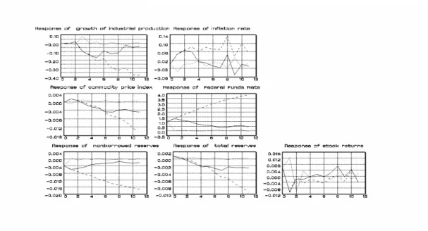
Figure 1 displays the dynamic response of excess returns, stock prices, and the growth rate of M2 from the change of federal funds rate (defined as a 100-basis-point increase in the federal funds rate). The solid line in the bottom-right panel of Figure 1 shows that excess returns decline due to unanticipated 100-basis-point increase in federal funds rate. If, however, investors predicted that the Fed was going to lower the target but in fact it did not, then the initial response of excess returns to this unexpected increase in the target is given by the dotted line, and shows is to increase in the first month. The bottom-right panel of Figure 1 shows that stock price reacts negatively to a surprise increase in the federal funds rate target, and the decline from the initial level is maintained over a 12-month horizon. This result is consistent with that of Bernanke and Kuttner (2005). In contrast, if investors predicted that the Fed would lower the target but in fact that target did not change, then stock prices delay one month to decrease.
5. Conclusion
This paper investigates the link between monetary policy and the stock market, in order to capture the relationship between the federal funds rate target and the stock market. We use a model that allows us to distinguish the effect on stock prices of
2 The effect of the weight wtin equation (10) is to ignore observations for which no change was expected, and to rescale positive or negative forecast errors into units comparable to equation (9).
unanticipated monetary policy arising from surprise increases in the funds rate target and unanticipated monetary policy arising from surprise“no change”occurrencesin the funds rate target. We use the ACH model to estimate the response of the stock market to these different unexpected monetary policy actions.
We find that stock prices react negatively to surprise change in the federal funds rate target. The long-run effect of the unanticipated monetary policy tightening is to decrease stock prices. This result is consistent with that of Bernanke and Kuttner (2005). In contrast, if investors predicted that the Fed was going to lower the target but in fact it did not, the response of stock prices are sticky for three months horizon.
Fig 1. Effect of
y
tj for j 0,1...11. Solid line shows the innovation of a forecast error in theVAR. Dashed line shows the innovation of that the Fed raised the federal funds target. Dotted line means the innovation of a forecast target change that failed to materialize. Different panes correspond to the different elements of y
6. Reference:
Bernanke, B., S. and Kuttner, K., N. (2005). What Explains the Stock Market’s Reaction to Federal Reserve Policy? The Journal of Finance, 6(3), p. 1221-1257
Guo, H. (2004). Stock Prices, Firm Size, and Changes in the Federal Funds Rate Target.
The Quarterly Review of Economics and Finance 44, 487-50
Hamilton, J.D., Jorda O. (2002). A Model of the Federal Funds Rate Target. Journal of Political Economy 110, p. 1135-1166.
Krueger, J. T., and Kuttner, K. N. (1996). The Fed Funds Futures Rate as a Predictor of Federal Reserve Policy, Journal of Futures Markets 16, p. 865-879
Rigobon, R., Sack, B. (2003). Measuring the Reaction of Monetary Policy to the Stock Market, The Quarterly Journal of Economics, May, 2003,
Smirlock, M., Yaitz, J. (1985). Asset Returns, Discounted Rate Changes, and Market Efficiency. Journal of Finance, 40, p. 1141-1158
Thorbecke, W. (1997). On Stock Market Returns and Monetary Policy, Journal of Finance 52, p. 635-654
Thorbeke, W. and Alami, T. (1994). The Effect of Changes in the Federal Funds Rate Target on Stock Prices in the 1970s. Journal of Economics and Business 46, p. 13-19
計劃成果評析 1. 完成之工作項目
a) Analyze the impact of changes in monetary policy on the stock market.
b) Decompose the monetary policy shocks based on the ACH (Autoregressive Conditional Hazard) model for the federal funds rate target.
c) Estimate the impact of these two different unexpected federal funds rate events on stock returns.
2. 評估是否可在國際期刊發表
本人在今年暑假前往 Texas A&M University, department of Economics, 與我的指導教授 Dr. Dennis, W. Jansen 合作完成此計劃, 預計今年年底將 此計劃投到國際的 Journal.