Learning Efficiency Improvement of Back Propagation Algorithm by Error Saturation Prevention Method
Hahn-Ming Lee, Tzong-Ching Huang and Chih-Ming Chen
Department of Electronic Engineering
National Taiwan University of Science and Technology
Abstract
Back Propagation algorithm is currently the most widely used learning algorithm in artijicial neural networks. wirh properly selection of feed-fnvard neural network architecture, it is capable of approximating most problems with high accuraq and generalization ability.
Howevec the slow conveeence is a serious problem when using this well-known Back Propagation (BP) learning algorithm in many applications. As a result, many researchers take effort to improve the learning eflciency of BP algorithm by various enhancements. In the research, we consider that the Error Saturation @S) condition, which is caused by the use of gradient descent method, will greatly slow down the learning speed of BP algorithm.
Thus, in the paper; we will analyze the causes of the ES condition m output layez An E m r Saturation Prevention (ESP) finction is then proposed to prevent the nodes in output 1ayerfi.om the ES condition. We ako apply this method to the nodes in hidden layers to a&& the learning terms. By the proposed methoak, we can not only improve the learning eflciency by the ES condition prevention but also maintain the semantic meaning of the energvfirnction.
Final&, some simulations are given to show the workings of our proposed method
Keywor&Back Propagation Neural Network, E m r Saturation(ES) Condition, Error Saturation Prevention(ESP) finction, Distance Entmpy
1. Introduction
The Back-Propagation (BP) algorithm [l] is a widely used learning algorithm in artificial neural networks [2]. It works well for many problems (e.g. classification or pattern recognition etc.) [1,3,4]. However, it suffers two critical drawbacks fiom the use of gradient-descent method one is the learning process often traps into local
minimum and another is its slow learning speed. As a result, there are many researches on them [5,6,7], especially for the learning efficiency improvement by preventing the Premature Saturation (PS) phenomenon [8,9]. The Premature Saturation (PS) means that outputs of the artificial neural networks temporally trap into high error level during the early learning stage. In the learning issues of PS phenomenon, researchers have designed many usable modifications to solve this phenomenon [10,11,12].
However, the proposed methods are limited to many assumptions and seem to be complex (will be detailed in the next subsection). In this research, we think that the Error Saturation (ES) condition [ l l ] is the main cause of
PS phenomenon. The ES condition means that the nodes in each layer of artificial neural network models have outputs near the extreme value 0 or 1, but with obvious differences between the desired and actual outputs.
Consequently, the learning term (signal) will be very small for the increment of weights or others parameters [13].
Therefore, we will use the Error Saturation Prevention (ESP) method to overcome the PS phenomenon and thus the learning convergence will speed up and the local minimum problem will be relieved. Besides, we keep the semantic meaning of used Mean Square Error (MSE) h c t i o n to rationalize the evaluation of error criterion.
2. Error Saturation Problem
In this paper, we focus on the efficiency improvement of BP algorithm by preventing the Error Saturation (ES) condition. This is because in our study we find that the main cause of the slow convergence in BP algorithm is the occurrence of the Premature Saturation (PS) phenomenon, and the ES condition will result in the PS phenomenon [11,12]. The PS phenomenon is shown in FIGURE 1. In this figure, we can check that during the occurrence of PS, the Mean Square Error (MSE) [l] will stay high in the early learning stage (iteration 140 to iteration 500) and will decrease gradually to lower error level after iteration 610.
In FIGURE 2, we give two examples to indicate the ES
condition. In CASE A, we can find that the desired output is 0 but the actual output is near 1 (i.e. the actual output is close to the extreme area). Under this condition, the ES will occur to result in the PS phenomenon and thus slow the learning efficiency. The similar condition will occur as shown in CASE B. Therefore, we can avoid the PS phenomenon by the ES prevention methods to improve the learning efficiency of Back Propagation Neural Network (BP") models.
0 5 I 1
- PS Occurrence -expected result
0
- - 2 : : g g s : :
iteration d e r (1110)
FIGURE 1. The. Premature Saturation (PS) phenomenon
CASEA: Desireaoutput(A) Actual output (A)
0 1 - 0 2 _,W' , , d < & Y W + , W < W
- 2
- (A) I Io'8 7
1 %Temc-a@)
CASE B
-
ouaul (B) D e S i d O U t p U t ( B )FIGURE 2. The E m r Saturation (ES) condition in nodes of output layer
3. Error Saturation Prevention Method
In this section, we will first analyze the causes of the Error Saturation (ES) condition and how the influence related to the learning efficiency of Back Propagation (BP) algorithm. Secondly, we construct an Error Saturation Prevention (ESP) function (e.g. parabolic function) to avoid the ES condition fiom output nodes. Then we apply the ESP method to the nodes in hidden layers with proper modifications.
3.1. Error Saturation Condition in Nodes of Output Layer
By gradient descent method used in BP algorithm, we can get the learning term for output nodes as:
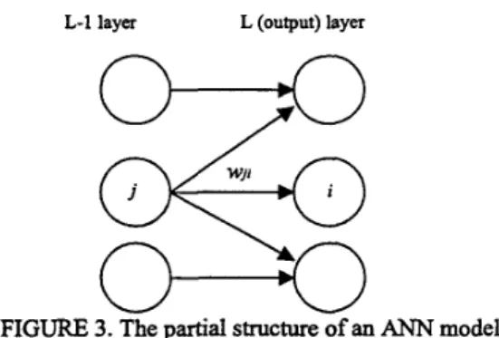
d i and Oi are the desired and actual values of the i-th output node, A w j i is the increment of the weight from the j-th node in L-1 layer to the i-th node in L layer, q is the learning rate, k is the temperature variable of activation function (assumed to be 1 in this paper), and oj is the output of the j-th node in G1 layer. The partial structure of an ANN model is shown in FIGURE 3.
L-1 layer L (output) layer
0-0
FIGURE 3.
0-0
The partial structure of an ANN model In order to analyze the learning term 6 in detail, we plot the learning term 4 as a function of delta value( d i - oi) and the actual output O i in FIGURE 4. In this figure, we can find that when the output oi is in extreme value close to 1 or 0, the learning term t i will be very small even the delta value ( d i -a) is large. That is, when the actual output Oi is in the extreme area, the learning term 6 is very small even the desired output d i is far from the actual output o f . Thus, w e must propose some methods to avoid the ES condition.
In order to understand the ES condition, we give the relationship of the learning term ti and learning factor oi x (1 -0) to illustrate the learning process dynamics. In FIGURE 5, we can see that the distribution of the learning term and learning factor. The desired output is assumed to be 1 to simplifi the representation. Since the learning term is determined by the learning factor oix (1 - oi) and the difference between the desired and actual outputs (delta value), the small quantity of the learning factor when the actual output is in the extreme area will decrease the learning term greatly even the delta value is large. Thus, it will delay the learning convergence a lot.
Awi = q x ( d i - oi) X k x oix (1 - oi) X O j = q X t i X O j (2) where 4 means the learning term for the i-th output node,
I actual output 0 1
deltavatuei-oi ;"i
FIGURE 4. The learning term ti of original BP algorithm
o m o o 8 o ~ o ~ o ~ o x o a os o n o ~ o . n o . 7 8 0 8 5 0 ~ 0 ~ d oapul 01
FIGURE 5. Distribution of the learning term ti when the desired value is 1
3.2. Using the ESP function to prevent the error saturation condition
In this paper, the Error Saturation Prevention (ESP) function is given to be a parabolic function as:
where a is scale term, n is exponent value and oi is the actual output of the i-th no& in output layer.
The examples of parabolic function are shown in FIGURE 6. In this figure, we can find that the parabolic function is indeed helpful to scale up the learning term when the actual output oi is near the extreme value 0 or 1, but it has little influence on the learning term when the actual output is at about 0.5. Therefore, we use the parabolic function as our ESP function. After including the ESP function, the learning term in equation (1) will become:
where ESP(a) is the used parabolic function a x (oi - 0.5)" as indicated in equation (3).
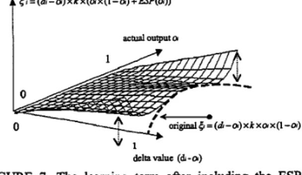
From FIGURE 7, we can find that the learning term {r will be enhanced when the actual output is in the extreme area. That is, including the ESP function to the learning term could help to overcome the degeneration of the learning Edctor ( a x (1 -a) ) when the actual output is near 0 or 1. Thus, the Error Saturation (ES) condition can be avoided.
ESP(Oi)=ax(a-O.5)" (3)
ti = (di -a) x k x ( a x (1 -a) + ESP(a)) (4)
-16X(a-O.5)'
8 X ( h - 0.5)'
16X(a-O.S)'
- _.__.
2 0 2
0 . - " " . , y w c m m
d ~ d d d o o o o o o
actual output a
FIGURE 6. Examples of parabolic function The parameters ( CL , n) are set to be (16,4), (8,6), and (16, 6) , respectively.
= (d -a) x k x(ax(1 -a) + ESP(ol)) actual output a
delta value (dl - a)
FIGURE 7. The learning term after including the ESP function
3.3. Effect of the ESP Method to the Energy Function
In our model, for the reason to overcome the degeneration of the learning factor OiX (1 -a) when the actual output oi is in the extreme area (i.e. the occurrence of the Error Saturation (ES) condition), we speed up the learning process by including the ESP function to the learning term t i . However, we should consider the effect of the ESP method to the energy function. Therefore, we will formulate the energy function after including our ESP
function. Then we analyze how the new energy function will contribute to the learning process.
In the Back Propagation learning algorithm, the Mean Square Error (MSE) function [l] is used as the energy function. We derive the energy function for training pattern p as:
E p = T X l N (di - O i ) 2
i = l
(5) where N is the node number of output layer, di and oi are the desired and actual outputs for node i in output layer.
Thus,
E = - - X ~ E ~ l P (6)
p=l
where E means the energy function (or called MSE
function), and P is number of training patterns. From the above energy function and the gradient descent method, the increment of weights is shown as:
JEP
&ji
Awji = - q X - = - q X ( o i - - ) X k X o i X ( l - o i ) X O j (7) where di and oi are the desired and actual outputs of the i-th output node, Awji is the increment of the weight from the j-th node in G 1 layer to the i-th node in L layer, q is the leaming rate, k is the temperature variable of activation function (assumed to be 1 in this paper), and Oj is the output of the j-th node in L-1 layer. The partial structure of an ANN model is shown in FIGURE 3. After including the ESP function, the increment of weight will become:
Awl'.. j i - - -7 x (oi - di) x k x (oi x (1 - oi) + ESP(0i)) x Oj (8)
As a result, we consider that the original energy function will be changed to:
E; = E ~ + E; (9) where E p is the MSE energy function for pattern p, g p is the added energy function after including our ESP fimction, and E; is the new energy function. Thus, we can rewrite the increment of weight Awji as:
For output node i , we derive the following equations
N
E% = z g p i i
where EA. is the MSE energy function of output node i for pattern p, and E'A. is the added energy function of output node i after applying the ESP method for pattern p.
From equation (1 0), (1 I), and (1 2), we could rewrite AW"ji
as follows:
(13) 3 ( E p i + E'pi)
=-qx ~
&ji
Also, from equation (8), we can easily derive the following term:
Aw'ji = -77 x (oi- di) x k x (oix (1 - oi) + ESP(0i))X Oj
= - q X +( -7 X (Oi - di) X k X ESP(0i)X Oj ) (14)
aWji
From equation (1 3) and (1 4), we have:
J (Epi + E;i)
aWji
= - q X
(15)
JEpi JE'pi)
= - q x- +( -7 x- )
&ji &ji
As a result, we can have the following equation:
(16) JE>i
aWji
- = (a - d) x k x ESP(0i) Xoj
Thus, by the integral method, chain rule and equation (3), we can derive the added energy function as:
(1 7)
+ 2 x d x (1 - d) - 2
From equation (17), energy function for patter p can be derived as:
1 N N
2 i I
E ; = E ~ + E ; , = - x z ( ~ ~ - o ~ ) ~ + z E ; ~ 1 N
2 i
= - x (di - Oi)2 +
Finally, the new energy function is:
. m
I '
El'=-x Z E ; P p = l
3.4. Applying the ESP method to the learning term in hidden layer
Without loss of generality, we assume the feed- forward neural network used is three layers, i.e. input- hidden-output layers. The learning term, which is propagated from output layer, is derived as:
i i
where 8 and 6 are the learning terms of the i-th output node (L layer) and the j-th hidden node (L-1 layer), w j i is the weight from the j-th node in L-1 layer to the i-th node in L layer, ne0 is the net value of the j-th node in L-1 layer, and oj is the output of the j-th node in G 1 layer.
The partial structure of an ANN model is shown in FIGURE 3.
From equation (20), we can find that the learning term for hidden layer will be small when the actual output is in the extreme area. This is the same as the Error Saturation (ES) condition in the output layer. However, there is no enough information about the desired output in hidden nodes during learning. Therefore, we can not directly handle the ES condition as the ESP method in output layer.
From equation (20), we could find the following facts:
2 3 Average The learning term for hidden layer can be divided into
two terms: one is the first derivative of activation fkction on the net input of the j-th node in hidden layer, i.e. the learning factor f ( n e 0 ) = W X ( ~ -@) , and the other is the learning term propagated from
3.16 3.71
4.30 4.57
3.48 3.83
N nodes in output layer C W j i t i .
i
Since we have enhanced the learning term in output layer, we will focus on the learning factor. In other words, we will overcome the degeneration caused by the learning factor to enlarge the learning term.
Therefore, for the improvement of the learning term in hidden layer, we consider that the learning term propagated fiom the output layer ( witi ) is appropriate. We could also include the ESP function to the learning term in hidden layer. By this way, we could speed up the learning convergence by the ES prevention. However, due to the unknown desired output in hidden layer, we could not apply the ESP function directly. Since we find that the learning term in nodes of hidden layer is too small, it may be enlarged hundreds of times if we apply the ESP function directly. This may lead the learning process to an oscillation state. Thus, we need properly control the effect of the ESP function when it is used to the learning term of hidden layer. We will use a constant factor (a real value) to the ESP function to make the enhancement of the learning term reasonable. Therefore, the learning term in the j-th hidden node willbe as:
N
i
N
6 = ~ w j i ~ x [ ~ x ( l - ~ ) + c x ~ ~ ~ ( ~ ) ] (21)
i
where C is a small real factor (e.g. 0.01)
Therefore, in our following experiments, we will first apply the ESP method to the learning term in nodes of output layer. Then we apply the ESP method to the learning term both in nodes of output and hidden layers.
We could find that the learning convergence speeds up as we apply the ESP method to output layer or both layers.
We will detail these results in the next section.
4. Experimental Results
In order to illustrate the workings of proposed methods, We use two classification problems with different complexity to verify our study in the Error Saturation Prevention (ESP) problem.
4.1. Experiment on Breast Cancer Data
This Breast Cancer data is obtained fiom the University of Wisconsin Hospitals [15]. There are nine attributes used to represent the pattern, and each pattern belongs to one of two classes: benign or malignant. The database consists of 367 data patterns originally [15].
Currently, it has been extended to 699 patterns. Since the original set (367 instances) is often referenced, we use the 367 patterns to be our training database. By considering the characteristics of the database, we use a 9 x 6 ~ 2 neural network model to solve the classification problem.
We set the node number of hidden layer to be 6 by the heuristic that the node number in hidden layer can be equal to the average of input (9) and output (2) node numbers.
In what follows, we divide the 367 patterns into training set (187 patterns) and testing set (180 Patterns), and use a=256 and n=8 to set our ESP function, i.e. the ESP ihction is set to be 256x(oi - 0.5)' . Besides, we set the learning rate to be 0.5 and the maximum learning iteration number to be 2000.
4.1.1. The experimental result of the ESP method in output and hidden layers
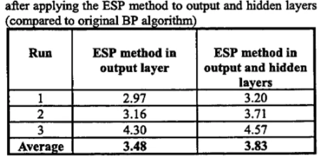
In order to show the applicability of the ESP method in output and hidden layers, a simulation result is shown in TABLE 1. In this table, we record the accelerating rates after applying the ESP method to output and hidden layers.
In this case, we can find that the improvement of the learning convergence will speed up to 3.83 times. Thus, the ESP method is applicable to learning process in hidden layers.
TABLE 1. The accelerating rates on Breast Cancer data after applying the ESP method to output and hidden layers
ESP method in ESP method in
4.2. Experiment on Fisher Iris Data
Run 1 2 3 Average
In this subsection, we use Fisher Iris data [14] as our second training database. The Fisher Iris database includes 150 four dimension features patterns in three classes (50 for each class). We use a 4 x 4 ~ 5 neural network model to solve the classification problem. In what follows, we divide the 150 patterns into training set (75 patterns) and testing set (75 patterns) and use a=4 and n=2 to set our ESP h c t i o n , i.e. the ESP function is set to be 4 ~ ( o i - 0 . 5 ) ~ . Besides, we set the leaming rate to be 0.1 and the maximum leaming iteration number to be 1600.
ESP method in ESP method in output output layer and hidden layers
1.36 1.57
1.47 1.89
1.72 2.05
1.51 1.84
4.2.1. The experimental result of the ESP method in output and hidden layers
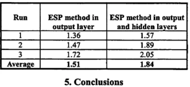
In order to show the applicability of the ESP method in hidden layers, a simulation result is shown in TABLE 2.
In this table, we record the accelerating rates after applying the ESP method to output and hidden layers. In this case, we can check that the improvement of the learning convergence will speed up to 1.84 times. Thus, the ESP method is also applicable to the learning term in hidden layers.
TABLE 2. The accelerating rates on Fisher Iris data after applying the ESP method to output and hidden layers
According to the previous analysis and simulations, we can draw the following advantages of applying our ESP methods:
(1) The ESP method is simple and intuitive to prevent the ES condition during the leaming process.
(2) The ESP method can speed up the leaming efficiency and escape &om the local minimum.
(3) Distance-Entropy can explain the phenomenon of accelerating learning and the ESP method could keep the semantic meaning of the used energy function.
References
[l] D. E. Rumelhart, G. E. Hiton, and R J. Williams, Learning Internal Representation by Error Propagation, Parallel Distributed Processing 1 (1 996)
31 8-362.
[2] R P. Lippmann , An Introduction to Computing with Neural Net, IEEE ASSP. MAG. (1987) 4-22.
[3] Y . L. Cun , Back-Propagation Applied to Handwritten Code Recognition, Neural Computing 1 (1989) 541- 551.
[4] M. Arisawa and J. Watata , Enhanced Back Propagation Learning and it’s Application to Business Evaluation, 1994 IEEE International Conference on Neural Networks, 1994, Vol. 1, pp. 155-160.
[SI N. Baba , A New Approach for Finding the Global Minimum of Error Function of Neural Networks, Neural Networks 2 (1989) 367-373.
[6] N. Baba , A Hybrid Algorithm for Finding Global Minimum of Error Function of Neural Networks, Proceeding of International Joint Conference on Neural Networks, 1990, pp. 585-588.
[7] S. Kollias, and D. Anastassiou , An Adaptive Least Squares Algorithm for the Efficient Training of Artificial Neural Networks, IEEE Transactions on Circuits and Systems, CAS-36, (1989) 1092-1101.
[8] J. E. Vetela and J. Reifinan , The Cause of Premature Saturation in Back Propagation Training, IEEE International Conference on Neural Networks, 1994, [9] Y. Lee, S. H. Oh, and M. W. Kim, The Effect of Initial Weights on Premature Saturation in Back Propagation Learning, Proceeding of International Joint Conference on Neural Networks, Seattle, WA., 1991, 101 K. Balakrishnan, and V. Honavar , Improving Convergence of Back-Propagation by Handling Flat- Spots in the Output Layer, Proceeding Of International Conference on Artificial Neural Networks, 1992, Vol.
111 Y Lee, S. H. Oh, and M. W. Kim , An Analysis of Premature Saturation in Back-Propagation Learning, Neural Networks 6 (1993) 719-728.
[12] J. E. Vetela and J. Reifinan , Premature Saturation in Back-Propagation Networks: Mechanism and Necessary Conditions, Neural Networks 10 (4) (1997) [13] S. H. Oh , Improving the Error Back-Propagation Algorithm with a Modified Error Function, IEEE Transactions on Neural Networks 8 (3) (1997) 799- 803.
[14] R Fisher , The Use of Multiple Measurements in Taxonomic Problems, Annals of Eugenics 7 (2) (1936) [15] 0. L. Mangasarian, R Setiono, and W. H. Wolberg ,
Pattern Recognition via Linear Programming: Theory and Application to Medical Diagnosis in: Large-scale Numerical Optimization (SIAM Publications, Philadelphia, 1990, pp. 22-30).
Vol. 2, pp. 1449-1453.
pp. 765-770.
2, pp. 1003-1009.
72 1-735.
179-1 88.