延長網路存活時間之適應性錨節點睡眠排程

國立臺灣大學工學院工程科學與海洋工程學系 碩士論文

Department of Engineering Science and Ocean Engineering College of Engineering

National Taiwan University Master Thesis

Maximizing Network Lifetime with Adaptive Beacon Duty Scheduling

延長網路存活時間之適應性錨節點睡眠排程

周元超

Yuan-Chao Chou

指導教授：丁肇隆 博士、張瑞益 博士

Advisors: Dr. Chao-Lung Ting and Dr. Ray-I Chang

誌謝

時光飛逝，兩年多的碩士生涯即將劃上句點。本論文的完成要感謝許多人的 協助與幫忙，首先最感謝我的指導教授丁肇隆博士及張瑞益博士。丁老師與張老 師帶領著懵懵懂懂的我進入了無線感測網路的專業領域，且總是不厭其煩地給予 許多建議與教誨；從兩位老師身上我學習到了做研究應有的精神，對學問的嚴謹 態度更是我學習的最佳典範，無論在生活上或是研究上皆受益良多，在此對兩位 老師致上由衷的謝意。另外還要感謝口試委員王家輝博士以及林正偉博士對於論 文的指導與建議，使得此論文能夠更臻完善。

感謝研究夥伴們在這兩年間的照顧與陪伴。感謝學長姐棨椉、忠原、育正、

孟翰、建彰、佳穎、任芯總能在我迷惘時適時地替我解惑；感謝一起打拼的戰友 承鴻、志永、孃瑩、景陽、肇普、昱瀚、仁峰、柏沇及學弟妹涵仁、億鑫、之盈、

東輝、禹豪在研究上的切磋砥礪及課餘的嘻笑打鬧，真的很開心能夠認識你們。

感謝弈勳、光宏、詠翔、書蔚、博範、彥廷，碩士生涯中有你們的相挺與陪 伴，為這兩年的研究生活提供源源不絕的活力。女朋友雅鈴在背後的默默支持更 是我前進的動力，沒有雅鈴的體諒、包容，相信這兩年時光描繪的會是幅很煎熬 的光景。

感謝我最親愛的家人們，李春菊女士與弟弟周華展，謝謝你們給我的支持與 包容，讓我能順利完成碩士學位。最後，謹以此篇論文獻給所有關心我的人。

周元超 謹致於 國立台灣大學 工科所 資訊與網路實驗室 中華民國 101 年 7 月

中文摘要

定位技術已在無線感測器網路(WSNs)中被廣泛應用於找出節點之未知位置。

一般在執行定位技術的過程中，會大量佈置錨節點(位置已知之節點)來協助推算其 他節點之位置；然而，同時啟動所有的錨節點並不能明顯地增加定位準確率，反 而會增加額外的能量成本與頻寬成本。在這樣的情況下，通常只需要同時啟動一 部分的錨節點就能達到準確率的要求，因此為了減少成本並延長網路存活時間，

本論文提出了可使錨節點自己安排工作周期的 Adaptive Beacon Duty Scheduling (ABDS)演算法。ABDS 會在線上即時量測錨節點位置之效益(在此位置啟動錨節點 後可能帶給定位準確率多少助益)，並且根據此量測結果挑出對定位準確率最有效 益的那些錨節點以啟動之，以將同時啟動的錨節點數量最小化。由於在前人的相 關研究中，並未實際去量測不同錨節點位置的不同效益，因此 ABDS 可更佳地適 應充滿無法預測之雜訊的真實環境。此外，為了在 ABDS 中精確地量測錨節點位 置之效益，我們觀察到錨節點對其覆蓋範圍產生的定位效能改善量事實上是非均 勻分布的，並提出了尚未被討論過的 Distribution-Adapted Grid (DAG)量測法以適 應此現象。與前人的方法相比，使用了 DAG 量測法的 ABDS 可以減少 10%的錨節 點使用量，並且延長 54%的存活時間。

關鍵字：無線感測器網路、定位、錨節點位置、工作排程、睡眠排程。

ABSTRACT

Within typical localization processes in wireless sensor networks (WSNs), beacon nodes which know their locations will broadcast information for localizing an unknown location. Although beacon nodes are massively deployed in the terrain, only a fraction of the beacon nodes are required to be active for satisfying accuracy requirement. Too many active beacon nodes may bring the system with little improvement on localization accuracy but waste of both costs of energy and bandwidth. To reduce the costs and prolong the system lifetime, we propose the Adaptive Beacon Duty Scheduling (ABDS) algorithm that can self-configure beacon duty. ABDS can turn on only the minimum set of beacon nodes in a same time according to the online-measured effectiveness of beacon locations (the effect of activating a beacon node at the location for improving localization performance), which is not considered in previous methods. Moreover, to precisely measure the effectiveness of beacon locations in ABDS, we need to realize the fact that a beacon node actually contributes non-uniformly distributed impact within its coverage. This Distribution-Adapted Grid (DAG) measurement that can adapt the non-uniformly distributed impact was not discussed in previous methods. Compared to the previous methods, ABDS with the usage of DAG measurement can reduce 10%

beacon usage and provide 54% longer lifetime.

Keywords: Wireless sensor networks, localization, beacon location, duty scheduling, sleep scheduling.

CONTENTS

口試委員會審定書... #

誌謝 ... i

中文摘要 ... ii

ABSTRACT ... iii

CONTENTS ... iv

LIST OF FIGURES ... vi

LIST OF TABLES ... viii

Chapter 1 Introduction ... 1

1.1 Motivation ... 1

1.2 Contributions ... 2

1.3 Thesis Organization ... 4

Chapter 2 Related Works ... 5

2.1 Beacon Duty Scheduling Algorithms ... 5

2.2 Related Works on the Measurement of the Effectiveness to Beacon Locations ... 8

2.3 Localization Algorithms ... 10

Chapter 3 Distribution-Adapted Grid Measurement ... 12

3.1 The Problem of Predicting the Effectiveness of a Beacon Location ... 12

Chapter 5 Evaluations ... 28

5.1 Environment Model ... 28

5.2 Evaluation of the DAG Measurement ... 29

5.2.1 Localization Algorithms ... 29

5.2.2 Simulation Parameters ... 30

5.2.3 Performance Metrics ... 30

5.2.4 Simulation Flow ... 31

5.2.5 Simulation Results ... 32

5.3 Evaluation of the ABDS algorithm ... 35

5.3.1 Energy Model ... 36

5.3.2 Localization Algorithms ... 36

5.3.3 Parameter Setting of Algorithms ... 37

5.3.4 Performance Metrics ... 39

5.3.5 Simulation Results ... 39

Chapter 6 Conclusions ... 46

REFERENCES ... 48

LIST OF FIGURES

Fig. 2.1. The state transition of STROBE. ... 6

Fig. 2.2. The state transition of E-STROBE. ... 7

Fig. 2.3. Illustration of the Max algorithm... 9

Fig. 2.4. Illustration of the Grid algorithm... 10

Fig. 3.1. Illustration of the positive effect and negative effect of adding a beacon node in connectivity based localization. ... 14

Fig. 3.2. Illustration of the impact of RSSI variation. ... 15

Fig. 3.3. The distribution of averaged improvements on localization error in the coverage of beacons. ... 16

Fig. 3.4. The averaged improvement distribution and weight distributions. ... 17

Fig. 3.5. The plot of Cauchy-form weight distribution with γ = 1. ... 18

Fig. 4.1. The state transition of ABDS... 24

Fig. 5.1. Solid circles mark the training data points. ... 30

Fig. 5.2. Flow chart of incremental beacon placement. ... 32

Fig. 5.3. The final beacon placement of Max, Grid, Greedy, and DAG in a 2-dimentional space. ... 33

Fig. 5.4. Performance of the measurements to incrementally place beacon nodes with connectivity based localization... 34 Fig. 5.5. Performance of the measurements to incrementally place beacon nodes with

Fig. 5.7. Mean localization error of ABDS, STROBE, and E-STROBE on connectivity-based localization. ... 42 Fig. 5.8. Active beacon ratio of ABDS, STROBE, and E-STROBE on connectivity-based localization. ... 43 Fig. 5.9. Snapshots of active beacon map of ABDS and Gribben’s method on MLE localization. ... 44 Fig. 5.10. Mean localization error of ABDS and Gribben’s method on MLE localization. ... 44 Fig. 5.11. Active beacon ratio of ABDS and Gribben’s method on MLE localization. 45

LIST OF TABLES

Table 5.1. Parameters and their values used in the simulations of incremental beacon

placement. ... 30

Table 5.2. Parameter settings of the energy model in the simulations of beacon duty scheduling algorithms. ... 36

Table 5.3. Parameters of ABDS and corresponding values. ... 38

Table 5.4. Parameters of STROBE and E-STROBE, and corresponding values. ... 38

Table 5.5. Parameters of Gribben’s method and corresponding values. ... 38

Table 5.6. Performance comparison of ABDS, STROBE, and E-STROBE. ... 41

Table 5.7. Performance comparison of ABDS and Gribben’s method. ... 45

Chapter 1 Introduction

1.1 Motivation

In wireless sensor networks (WSNs), both network operations and most application level tasks require the help of localization algorithms to acquire knowledge of the physical locations of devices [1], [2], [3], such as event detection [4], routing [5] and coverage [6]. These localization algorithms usually make use of beacon (anchor) nodes, whose locations are known prior to perform the localization algorithm, for the purpose of estimating unknown locations of other sensor nodes [7], [8], [9]. Locations are then computed by proximity-based approaches, range-based approaches, or angle-based approaches [3] according to the information gathered from beacon nodes. The accuracy of location estimations may increase as a function of the number of covered beacon nodes. However, deploying too many beacon nodes brings costs of bandwidth and excessive power consumption with limited improvement on localization accuracy, and thus leads to shortened system lifetime. Therefore, a scheduling scheme which considers effectiveness of beacon locations (the effect of activating a beacon node at the location for improving localization performance) to schedule their duty cycle is useful for the purpose of increasing system lifetime while maintaining required localization accuracy. Most of existing scheduling algorithms are designed for maintaining sensing coverage or connectivity [10], [11], [12], [13]. Only a few papers are proposed to schedule beacon duty cycle, such as [14], [15], [16], [17]. However, most of them did not consider the impact of beacon node deployment, which has been identified as a significant factor that has strong influence on localization accuracy [18]. Moreover, they are designed to control the density of active beacon nodes. It is not friendly for users (in

this thesis, “users” are the people that apply a localization algorithm and a beacon duty scheduling algorithm to construct their localization system) to set a desired control point of localization accuracy. In [15], the authors propose a scheduling algorithm that considers theoretical location error estimation of beacon nodes, which is not able to adapt noisy environment in real world. In addition, it is specifically designed for distance-based localization and cannot be applied to other kinds of localization algorithm.

1.2 Contributions

As demonstrated in [18], a good beacon deployment can meet the localization performance requirement with fewer active beacon nodes. The costs of power and bandwidth can be reduced and the system lifetime can be prolonged if only fewer beacon nodes are active to strobe at the same time. In real world, noise is inevitable and unpredictable in the localization systems. Therefore, a scheduling method that can dynamically adapt the noisy environment is necessary for both the purposes of selecting minimum active set of beacon nodes to reserve energy and controlling localization accuracy to user defined control point.

In this thesis, we propose Adaptive Beacon Duty Scheduling (ABDS) algorithm which can prolong system lifetime while maintaining required localization accuracy.

The fundamental limitation of previous approaches is that they basically miss the actual impact of beacon location in real world. They do not take into account effectiveness of

consumption and packet traffic. Therefore, an improved measurement to the effectiveness of beacon locations that can more precisely dig out beacon nodes with better effect on localization is also developed in this thesis. Empirical manners that can adapt to terrain conditions are favored in real world because it is hard to build a model to fit a certain environment. To our knowledge, little literatures have been published into this area, such as [18], [19]. In [18], Max and Grid take localization error and regional cumulative localization error as the measurements to the effectiveness of beacon locations respectively. In [19], Greedy addresses the beacon placement as a set cover problem, and takes coverage degree as the measurement to the effectiveness of beacon locations. We observed that after activating an additional beacon node, the impact on localization performance does not uniformly distribute in its coverage. The region closer to the beacon has better chance to reduce localization error. This phenomenon was not discussed in previous studies and should be overcome to get a more precise measurement to the effectiveness of beacon locations. Consequently, we improve the measurement in Grid and propose the Distribution-Adapted Grid (DAG) measurement for designing minimum active beacon nodes deployment in beacon duty scheduling.

The scheduling algorithm meets following design goals.

 Maximize system lifetime

 Distributed

 Adaptive to noisy environment in real world

 Can be applied to any types of localization algorithm

 User defined localization accuracy requirement

1.3 Thesis Organization

The remainder of this thesis is organized as follows. Chapter 2 discusses related researches about beacon duty scheduling, measuring effectiveness of beacon locations, and localization algorithm. The DAG measurement is developed in Chapter 3. In Chapter 4, the ABDS algorithm is developed. Chapter 5 shows the performance evaluation of proposed methods. Finally, the conclusions are made in Chapter 6.

Chapter 2 Related Works

In this section, related works are presented in three parts. Section 2.1 introduces existing algorithms for scheduling duty cycle of beacon nodes. Two referred works on the measurement to the effectiveness of beacon locations are introduced in Section 2.2.

To explain the phenomenon of non-uniformly distributed impact produced by beacons on localization, two localization algorithms are introduced in Section 2.3.

2.1 Beacon Duty Scheduling Algorithms

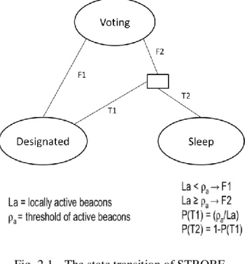
In [16], STROBE algorithm is proposed to schedule beacon duty by tuning the operation beacon density. STROBE adopts a scheduled rendezvous scheme that activates all beacon nodes up at the same time. Beacon nodes then exchange the information of activation distribution with their neighbors. If the local density of active beacon nodes is under a user defined threshold, the beacon node remains active for transmitting beacon signal to maintain the active density requirement. If the density exceeds the threshold, the beacon node takes a probability of excess density (e.g., the threshold is 7 and the density for now is 9, then the probability is (9-7)/7) to sleep for the purpose of reducing density to the threshold. The state transition of STROBE is shown in Fig. 2.1.

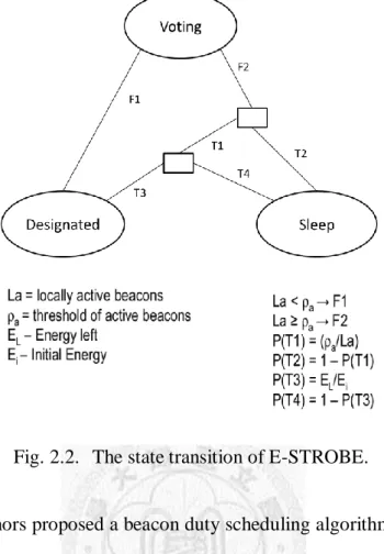
In [17], in order to spread energy consumption over beacon nodes for loading balance, the authors proposed E-STROBE, which extends STROBE to consider the ratio of remaining energy as a factor in making decision to active or sleep. E-STROBE takes a probability of the ratio of remaining energy before entering into the active state.

Fig. 2.2 illustrates the state transition of E-STROBE.

Fig. 2.1. The state transition of STROBE.

In [14], the authors proposed a beacon duty scheduling algorithm inspired by Span [10]. The algorithm fuses the parameters of active density and remaining energy into a delay time. After a beaconing or sleeping period, each beacon node transits the state to calculate the delay time. When the delay timer expires, the beacon node checks the active density in its neighborhood. If the density does not satisfy a user defined threshold, the beacon node is activated to transmit beacon signal, otherwise it is turned off to sleep for reserving energy.

In [15], the authors of [14] improve their scheduling algorithm by considering the theoretical location error estimation [20] rather than the density of beacon nodes as the design parameter. The location error estimation, which is specifically designed for range-based localization algorithms, makes use of the CRLB that places a lower bound on the variance of unbiased estimators [21] and was derived for position estimation in [22]. If the estimated location error is above a user defined threshold, the beacon node is

Fig. 2.2. The state transition of E-STROBE.

activated to transmit beacon signal, otherwise it is turned off to sleep.

2.2 Related Works on the Measurement of the Effectiveness to Beacon Locations

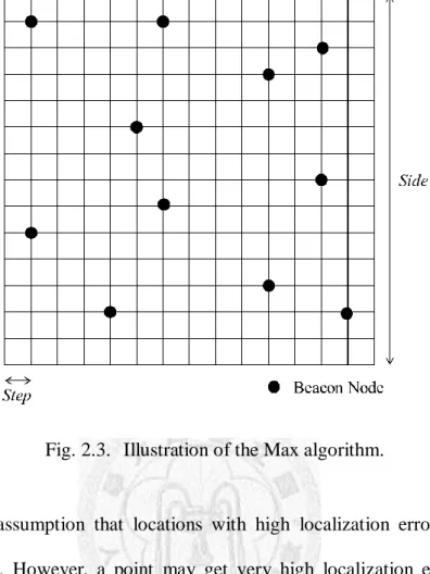
In the Max algorithm [18], localization error (distance between estimated location and actual location) is taken to be the measurement to evaluate the effectiveness of a beacon location. The idea is that a location with larger localization error has larger room to improve localization performance and thus larger benefit gained by placing a beacon node on this location. By this measurement, beacons are placed in an incremental manner. Every time the effectiveness for localization performance at each point on the terrain is measured, and then an additional beacon is placed on the point with highest localization error. The steps to incrementally place beacons are described as following.

1. The environment terrain is divided into Step× Step squares.

2. Measure the effectiveness for reducing localization error at each point in the terrain that corresponds to a square corner.

3. Add an additional beacon at the point that has the highest measurement value among all points.

Fig. 2.3 illustrates the Max algorithm.

There is an assumption that locations with high localization error are spatially correlated in Max. However, a point may get very high localization error while the localization error at other points close to it remains low, and that adding an additional beacon affects the localization error on its nearby region not just the point where it is placed. Based on these observations, the authors proposed the Grid algorithm [18]. In Grid, a 2-dimensional rectangular sliding window called “grid” with side length gridSide=2R (R is the ideal radius of communication range) is set up and the

localization errors that lie in the grid are summed up to be the measurement at the center of this grid. The Grid measurement is taken to incrementally place beacons (by the steps described in Max beacon placement algorithm) in the Grid algorithm, as illustrated in Fig. 2.4

Fig. 2.3. Illustration of the Max algorithm.

It is a proper concept in Grid to cumulate regional localization error as the measurement to decide beacon locations. However, the Grid measurement overestimates the ability of a beacon to improve the localization performance on its nearby region in such a way that beacon node resources are misspent. The observation of this phenomenon and the proposed measurement to more precisely estimate regional localization impact are described in Chapter 3.

2.3 Localization Algorithms

Connectivity based localization. Connectivity based localization [8] adopts beacon Fig. 2.4. Illustration of the Grid algorithm.

beacon nodes, the blind node estimates its location (X_est, Y_est) as the centroid of the locations of all connected beacon nodes with the centroid formula shown in Eq. (2.1).





, _{est est} X X^N Y Y^N

X Y

N N

 

 

  

  (2.1)

Pattern matching localization. Based on taking received signal strength indices

(RSSIs) from beacons as the feature vector of a location, pattern matching localization estimates an unknown location with similar features [7]. This localization algorithm consists of two phases, namely training phase and locating phase. In the training phase, RSSIs on training locations are recorded with the location coordinates, and the collected data are used to build a localization model. In the locating phase, a blind node collects the RSSIs from beacons to be the feature vector of its location, and then inputs the feature vector into the localization model to estimate the unknown location.

Chapter 3 Distribution-Adapted Grid Measurement

In order to select out a minimum set of active beacon nodes with best effect on localization to satisfy the requirement of localization accuracy, a precise measurement to the effectiveness of beacon locations is necessary for efficient beacon duty scheduling. Researchers have proposed methods for the measurement in beacon placement algorithms [17], [18]. However, the Grid measurement has a defect and solutions have not been proposed, hence for better predicting the effectiveness of beacon locations, an improved measurement (i.e., Distribution-Adapted Grid or DAG) is proposed in this chapter.

3.1 The Problem of Predicting the Effectiveness of a Beacon Location

This thesis addresses the problem of predicting the effectiveness of a beacon location as follows. A deployment B that consists of n active beacon nodes _aⁿ { ,...,b_a1 b_aⁿ} with Cartesian coordinates {z¹_a 







 



mean localization error _mean on T with a certain active beacon deployment B_aⁿ is

 

0 0

2

( , ), ( )

( 1)

side step side step

n a

x y

n

mean a

x y B

B side

step



  ^{ }



 

. (3.1)

A measurement to the effectiveness of beacon locations ( ,z B_aⁿ) takes the active beacon deployment and measurable information of the location (e.g., measured RSSIs, measured distances, packet receiving ratios, etc.) as inputs to predict a location’s effectiveness for activating a beacon node to reduce the mean localization error on the terrain. That is, for a perfect measurement ( ,z B_aⁿ), given an existing beacon deployment B_aⁿ and ^{Ban1 }



 



( _n 1,B_aⁿ) _mean

 z _   , (3.2)

where _mean_mean(B_aⁿ)_mean(B_a^n1). (3.3) The precision of a ( ,z B_aⁿ) can be evaluated by the reduction of mean localization error produced via activating a beacon node at the location z with maximum _i

( ,_i B_aⁿ)

 z , i.e.,

 

1 1

( )

( , ) ( ) ( , (arg max ( , )) )

n

i a

n n n n n n

mean a a mean a mean a a i a

T B

B B B B b B

 ^   ^ 

 

 

 

    

 

 ^{z z} z  . (3.4)

3.2 Developing Distribution-Adapted Grid Measurement

According to the definition proposed in Section 3.1, the measurements used in Max and Grid can be written down as Eq. (3.5) and Eq. (3.6).

( , ⁿ) ( , ⁿ)

Max Ba Ba

 z  z . (3.5)

 

. .

. .

( , ) ( , ),

R R

x y

step step

n n

Grid a a

R R

x x y y

step step

B x y B

 

 

   



 

z z

z z

z (3.6)

Although the Grid measurement _Grid can be used to design appropriate beacon locations when beacon density is low, it starts to mismeasure the effectiveness of beacon locations when the beacon density rises and the ability of a beacon to improve the localization performance on its nearby region decays. To consider regional localization error is reasonable. However, we observed that the improvement on localization performance in the coverage of a beacon node does not distribute uniformly. The location where an additional beacon is activated holds best effect of improving localization accuracy. This was observed from both connectivity based localization and pattern matching localization.

For the case of connectivity based localization, the estimated location of a blind node with unknown location is the centroid of connected beacons. Due to the fact that activating an additional beacon that covers it will pull the estimated location to be closer to the new beacon, both positive effect and negative effect on the nearby region of a new beacon are possible to occur, as illustrated in Fig. 3.1. Therefore, only the locations of added beacons always gains improvement on localization performance.

For the case of pattern matching localization, the information of locations hides in RSSI features, hence the pattern matching localization performs better with more dissimilar RSSI features. According to the path loss model without the noise term, signal strength decreases with the increase of distance in a logarithmic fashion [23], as described in Eq. (3.7).

0

0

( )

10 log( ) ( )

r

r dB

P d d

P d  d

 

   

  , (3.7)

where Pr(d) is the mean received power at distance d, Pr(d0) is the received power at the close-in reference distance d0 and β is the environment-dependent parameter. The closer the distance between transmitter and receiver is, the greater the change of RSSI is. Fig.

3.2 illustrates this phenomenon.

Even if noise exists in the path loss model in real world, a location closer to the beacon has better chance to get a more distinguishable feature and thus better performance of pattern matching localization.

To confirm our observations, Fig. 3.3 shows the distribution of averaged improvements on localization error in the coverage of beacons over iterations in an incremental beacon placement. The point where a beacon is placed holds best effect to improve localization performance as our inference. The ability of a beacon to improve the localization performance on its neighboring region decreases with the increase of the distance from the beacon.

Fig. 3.3. The distribution of averaged improvements on localization error in the coverage of beacons.

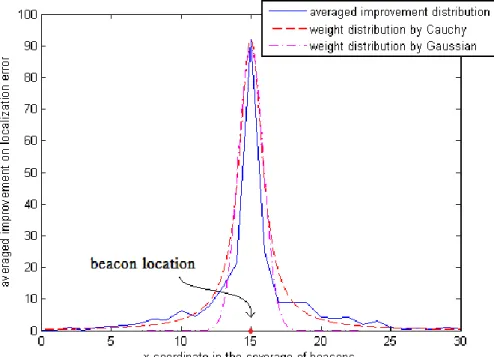
the beacon coverage. As a result, the Distribution-Adapted Grid (DAG) measurement that can more properly measure the effectiveness of a beacon location is proposed in this thesis. Two famous centralized distributions, namely Cauchy and Gaussian, are considered to weight the regional error. Fig. 3.4 shows the lateral view of the improvement distribution shown in Fig. 3.3 and the weight distributions generated by Cauchy and Gaussian.

The Cauchy distribution is more approximative to the improvement distribution, and thus adopted to generate a centralized weight distribution to adjust the cumulation process in regional localization error to fit the improvement distribution in beacon coverage. The three-parameter Cauchy distribution is defined by





0

; , ,

( )

f x x I I

x x

 



 

    , (3.8)

where 𝛾 is the scale parameter which specifies the half-width at half-maximum, I is the height of the peak, and x₀ is the location of the peak of this distribution. Because the

Fig. 3.4. The averaged improvement distribution and weight distributions.

purpose of this distribution function here is to generate weight distributions, I is taken with 1, and (x-x0) can be replaced by the distance D between beacon location and the location which contributes its localization error to cumulate regional error. Accordingly, the Cauchy-form weight distribution function here is defined by





w D ( )

D

 

 

 . (3.9)

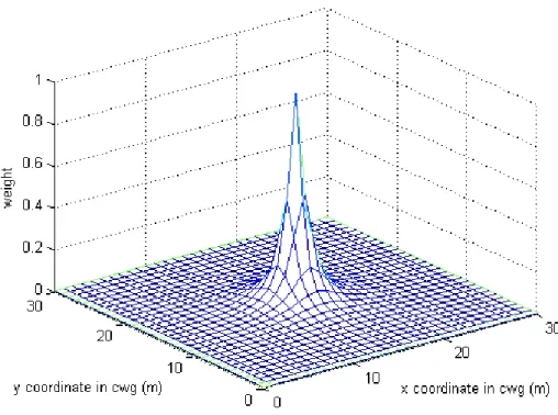
Fig. 3.5 demonstrates a weight distribution generated by Eq. (3.9) with γ = 1.

To compute the DAG measurement, the weight distribution is applied to weighting the regional localization error. A 2-dimensional rectangular sliding window called

Fig. 3.5. The plot of Cauchy-form weight distribution with γ = 1.

   

. .

. .

( , ) ;

( , ) ( , ),

R R

x y

step step

n n

DAG a a

R R

x x y y

step step

B w x y  x y B

 

 

   

 



 

z z

z z

z z . (3.10)

In this chapter, we observe that a beacon node contributes a centralized-distributed localization improvement in its coverage. Its location holds the best effect to reduce localization error, while the amount reduced on neighboring region decreases with the increase of the distance from the beacon node. It can result bias in measuring the effectiveness of a beacon location if one does not consider the regional error or consider the regional error as uniformly distributed. According to the impact distribution shown in Fig. 3.3, we select the Cauchy distribution, which can fit the distribution best, to design the DAG measurement. DAG can consider the real impact distribution in a proper manner and thus measure the effectiveness of a beacon location more precisely.

Previous measurements were implemented in the manner of incremental beacon placement (i.e., given an initial beacon deployment, then iteratively place a beacon node at the location with greatest measured effectiveness). Therefore, to evaluate and compare the performance of our DAG with previous methods, it will be applied to design beacon deployments by incrementally placing beacon nodes in Chapter 5.

According to Eq. (3.2), a measurement is more precise if the mean localization error reduced by activating an additional beacon node with biggest value is greater.

Accordingly, the localization accuracy can be achieved with fewer active beacon nodes.

Chapter 4 Adaptive Beacon Duty Scheduling

Most of previous scheduling algorithms that consider beacon duty cycle take active beacon density as the design parameter to adjust beaconing duty and be provided for users to set desired control points, such as [14], [16], [17]. Nevertheless, two drawbacks majorly exist in such manners.

 They do not consider the impact of beacon location, which has been identified as a significant factor for localization accuracy [18]. The algorithms make beacon nodes detect active neighbors and compute local density (density in their radio coverage) when the beaconing (sleeping) timers expire, and then select beacon nodes to be turned on or turned off to satisfy the density requirement according to random factors rather than the impact of beacon nodes. Therefore, some beacon nodes located at the locations without any benefit on reducing localization error (e.g., the location near to an active beacon node) may be turned on to transmit beacon signal, and thus the costs of energy and bandwidth are wasted.

 Density is not an intuitional parameter for setting a desired control point.

Expressly, one wants to set the requirement of localization accuracy when he is building a localization system with a beacon duty scheduling algorithm.

The relation between density and accuracy depends on the localization algorithm used, environmental factors, and power settings of beacon nodes. It

In [15], a location error estimation method is introduced to evaluate the localization error against probability at a beacon location [20], [21], [22]. However, the scheduling algorithm attempts to assign more beacon duty to the beacon nodes placed at a location with lower estimated error. In the formula of delay time [15],

( ) 1

max

i r

i

t

d P E

delay R T

D E

     

    

    

  , (4.1)

a smaller ratio term of location error estimation will result in a shorter delay time, and thus make the beacon node earlier to wake up to preempt a beacon duty. As a result, beacon nodes located at the locations with less effectiveness on reducing localization error are easier to be turned on, hence the costs of energy and bandwidth rise. Although the estimation formula considers two environment-dependent parameters, they are fixed that do not adapt to the variations in environments. Furthermore, the environment-dependent impact of beacon locations is not considered The Gaussian noise variable introduced in the estimation is used to describe the spatially distributed noise [23], whereas the formula considers it in a time-dependent manner. Moreover, the location error estimation is derived for distance-based localization algorithms, hence cannot be applied to localization algorithms in other types.

To effectively reduce cost of beaconing and maximize system lifetime, the impact of beacon locations must be adaptively considered in scheduling beacon duty cycle. In this chapter, we use the DAG measurement developed in Chapter 3 to design an adaptive beacon duty scheduling algorithm.

4.1 Problem of Beacon Duty Scheduling

Beginning from following the notations defined in Section 3.1, we introduce other

network N consists of beacon nodes b in ⁱ BN that know their locations





beacon nodes B_aⁿ B to transmit beacon signal in a period T , while the amount of _B mean localization error _mean(B_aⁿ) remains below a distance threshold D. Other beacon nodes B_s^m B in the sleeping state turn off their radio transceiver to reserve energy. Neighbors of a beacon node bⁱ is denoted by





( ) ( )

i j

i j

r b b threshold

N b  b B P d P , which are the beacon nodes that receive the signal from b with RSSI greater then received power threshold ⁱ P_threshold.

4.2 Developing Adaptive Beacon Duty Scheduling

In this section, we propose Adaptive Beacon Duty Scheduling (ABDS) algorithm, which attempts to achieve following design goals.

 Maximize system lifetime: A beacon duty scheduling algorithm must be able to

find out redundant beacon nodes that have less effectiveness on reducing localization error and make them sleep to reduce power consumption.

 Distributed: The scheduling algorithm should be distributed that needs only

local information obtained by 1-hop broadcast from neighbors for two reasons:

WSNs are usually constructed in an ad-hoc manner, hence it should be able to adapt churn (nodes joining or leaving) without coordination provided by a

system into the working environment (e.g., measure the RSSIs at various distances to evaluate noise strength) in real world. In addition, the environmental conditions may change and disturbances may occur when the system is working. Therefore, an on-line adaptive manner is attractive in this scenario.

 User defined localization accuracy requirement: The mean localization error

in a terrain should be maintained to satisfy a required threshold. The intuitional parameter for setting requirement for a localization system is localization error. Accordingly, a beacon duty scheduling algorithm must be able to control localization error.

ABDS mainly consists of decision stage and execution stage. In the decision stage, information about local mean error, remaining energy, and effectiveness on reducing localization error are computed and exchanged between neighboring beacon nodes in B. After making the decision, beacon nodes join the active beacon set B to take the _aⁿ duty to transmit beacon signal or join the sleeping beacon set B_s^m to reserve energy in the execution stage. When the timer of execution period expires, a decision is remade for rotating the beacon duty. To apply DAG measurement _DAG( ,z B_aⁿ), localization errors at neighboring beacon nodes are required, and therefore the decision stage is composed of three phases. First, activity information about one-hop neighbors is collected. The localization error at beacon nodes’ location can thus be computed and exchanged between neighboring beacon nodes in the second phase. With the knowledge of localization errors on one-hop neighbors, beacon nodes can then locally compute DAG measurement to evaluate their effectiveness on reducing localization error. The value of DAG measurement is fused with the ratio of remaining energy and exchanged

in the third phase. Finally, the decision can be made according to the comparison of active priority with neighbors. The state transition of ABDS can be illustrated by Fig.

4.1.

Follows describe the detail of each phase in ABDS.

 Decision stage-Beacon Signal (DBS) phase: All beacon nodes bⁱB start with stateⁱ active and set a timer T_DBS . Active beacon nodes b_aⁱB_aⁿ broadcast advertisements in a beaconing interval T to announce their _B activity. All b turn on the radio transceiver to listen for advertisements from ⁱ their neighboring active beacon nodes and construct active neighbor list

 

( ) ( i j)

i j n

a a a r threshold

N b  b B P d P . When the timer T_DBS expires, all b ⁱ Fig. 4.1. The state transition of ABDS.

active neighbor list N b_a( )ⁱ and compute localization error of ( ,zⁱ N b_a( ))ⁱ , and then broadcast the value of ( ,zⁱ N b_a( ))ⁱ to neighboring beacon nodes in

( )ⁱ

N b in the beaconing interval T_B and listen for





 Decision stage-Active Priority (DAP) phase: All beacon nodes b set a timer ⁱ TDAP . According to the localization errors distributed in N b( )ⁱ , i.e.





  ^{ }

( )

, ;

( ) ( , ( ))

j

i j

i

i j j

DAG b b a threshold

b N b

N

w d b

   









z z , (4.2)

where _threshold is the user defined mean error threshold. A fused active priority AP can then be computed by

 

( ) 1

i

i i r

DAG i

i

AP ef E ef

 ^{ }E ^{ }

     

   

 

z , (4.3)

where E is the remaining energy of _rⁱ b , ⁱ E is the initial energy of _iⁱ b at ⁱ time 0, and ef in the range





i r i i

E

E be considered. For a b with ⁱ

i 0

AP  , it has higher priority to take a beacon duty with higher AP for the ⁱ reason of activating beacon nodes as few as possible. Otherwise for APⁱ 0, it has higher priority to sleep with higher AP (less effect on reducing ⁱ localization error) for inactivating beacon nodes as many as possible.

Therefore, the energy ratio term is considered in this way to make a beacon

node with less energy get a chance to sleep more easily. All b broadcast ⁱ their AP in ⁱ T and listen for _B





 

 

( )

( , ( )) ( )

j i i

j j

a

b N b b

i

mean i i

N b N b b



  ^



. (4.4)

If the state of b is active and the local mean error ⁱ _meanⁱ is smaller than

threshold

 , b may be a redundant active beacon node, hence it then compare ⁱ

its AP with other neighbors that have same conditions (ⁱ state^j active and

j

mean threshold

  ) and set its state to be asleep if AP is the greatest one. ⁱ

Otherwise, if the state of b is asleep and the local mean error ⁱ _meanⁱ is greater than _threshold, b is a candidate to be active to reduce localization ⁱ error, hence it then compare its AP with other neighbors that have same ⁱ conditions (state^j asleep and _mean^j _threshold) and set its state to be active if AP is the greatest one. This can be expressed by ⁱ

   

i i i

mean threshold

state asleep state active   

 





       (4.5)

and

  



i i i

mean threshold

state active state asleep   

and broadcasts beacon signal in next stage. Otherwise, if stateⁱ asleep, b ⁱ joins B_s^m and sleep for reserving energy.

 Execution stage-Beacon Only (BO) phase: All b_aⁱB_aⁿ set a timer T_BO at the start time in BO. All b_aⁱ periodically transmit beacon signal at intervals

T and sleep for the remainder of the intervals. When the timer B T_BO expires, all b_aⁱ transition back to the DBS phase.

 Execution stage-Sleep (SL) phase: All b_sⁱB_s^m set a timer T at the start _SL time in SL and then go to sleep. When the timer T expires, all _SL b _sⁱ transition back to the DBS phase.

Chapter 5 Evaluations

Simulations and evaluations of proposed DAG measurement and ABDS algorithm are carried out in MATLAB 7.11.0 with a wireless sensor network simulated by the typical shadowing propagation model [23]. To confirm our observations in Section 3.2, the DAG measurement is evaluated on both connectivity based localization and pattern matching localization. To compare with previous methods, the ABDS algorithm is evaluated on connectivity based localization for the comparison with STROBE and E-STROBE, and on maximum-likelihood estimator (MLE) for the comparison with Gribben’s method in [15].

5.1 Environment Model

The log-normal shadowing model is adopted to generate simulated terrains with real-world noise condition. Based on the path loss model as defined in Eq. (3.7), the Gaussian random variable with zero mean and standard deviation _db (shadowing deviation) Xdb N





 

 

r

dB

r dB

P d d

d X P d

    

  

   

   

 

. (5.1)

5.2 Evaluation of the DAG Measurement

To be compared with previous measurements proposed in beacon placement algorithms, proposed DAG measurement is applied to incrementally place beacon nodes to design beacon deployments. Not only referred works in [18], but also a recent empirical method namely Greedy [19], which allows adaptation to terrain conditions and takes connected beacon density as the measurement to incrementally place beacons to design beacon deployment, was carried out in simulations and compared with proposed DAG measurement.

5.2.1 Localization Algorithms

The incremental beacon placement process was performed on connectivity based localization and pattern matching localization. Connectivity based localization algorithm computes the centroid of connected beacons as the estimated location for a blind node. If the mean received power exceeds the receiving threshold P_threshold, a blind node is identified as connected with the beacon node. Subsequent to computing mean received power by Eq. (5.1), connectivity is evaluated by applying following condition,

r( ) threshold

P d P . (5.2)

In the pattern matching localization algorithm, the k-nearest neighbor (KNN) algorithm, which uses Euclidian distance to find out k nearest patterns and select the mode to be the output, is applied to extract signal feature of locations. This localization algorithm comprises training phase and locating phase. The half of data points (feature vector of signal strengths and corresponding location coordinate) are uniformly chosen to be the training data set to establish feature database amid the training phase. The training data selection is illustrated in Fig. 5.1. In the locating phase, an unknown location is

estimated by the KNN operation on its signal strength feature.

5.2.2 Simulation Parameters

The values of log-normal shadowing model parameters are chosen from the ranges of their typical values in indoor environments [23]. Pr(d0) is obtained by the experiment in an indoor environment. The parameters and corresponding values used in this simulation are summarized in Table 5.1. They do not exactly reflect the details of a real environment, but are representative of the range of environments in which the algorithms may be applied.

Fig. 5.1. Solid circles mark the training data points.

Table 5.1. Parameters and their values used in the simulations of incremental beacon placement.

used to evaluate and compare the performances of various measurements used to design beacon deployment. However, according to the fact that the locations of training data are known, for the simulations with pattern matching localization, only the data points which are not in the training data set are chosen to examine the mean localization error.

Therefore, following equation is used to examine the mean localization error in the pattern matching localization.

 

mod 2

0 0

2

( , 2 mod 2), ( )

1 2

side step side step x

n a

x y

n

mean a

x y x B

B

side step







 



   

   

  

 

 

(5.3)

5.2.4 Simulation Flow

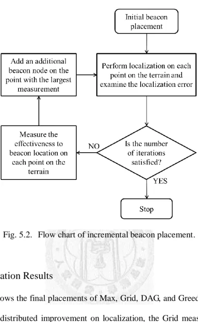
DAG, Max, Grid, and Greedy were evaluated in the simulations carried out in MATLAB to incrementally place beacons (by the steps described in Section 2.2) respectively. In each of simulation rounds, initially 20 beacons are randomly placed in the terrain. After examining the localization errors on the terrain, the location without a beacon that has highest measurement value is chosen to place an additional beacon.

Then the mean localization error is re-examined. Fig. 6 shows the flow chart to illustrate the flow of incremental beacon placement. There is a random factor in the initial state (i.e., random beacon placement). To characterize the statistical significance of our simulation results, each simulation executes for 10 times with different random initial beacon placements.

5.2.5 Simulation Results

Fig. 5.3 shows the final placements of Max, Grid, DAG, and Greedy. According to the centralized-distributed improvement on localization, the Grid measurement overly expects the ability of a beacon node to reduce the localization error in neighboring region. Therefore, many beacon nodes will be designed to place at locations with no any benefits on localization. This overestimation flaw of Grid causes a locally dense placement behavior that extremely squanders on beacon resource.

Fig. 5.2. Flow chart of incremental beacon placement.

Fig. 5.4 and Fig. 5.5 show the simulation results of incrementally placing beacons on connectivity based localization and pattern matching localization respectively. The averages and 95% confidence intervals are plotted in the figures.

Fig. 5.3. The final beacon placement of Max, Grid, Greedy, and DAG in a 2-dimentional space.

Fig. 5.4. Performance of the measurements to incrementally place beacon nodes with connectivity based localization.

As shown in Fig. 5.4, Grid provides better performances than Max at early placement stage. That confirms the idea of considering regional localization error. However, because of the locally dense placement behavior, Grid quickly starts to converge and provides the saturated localization performance much worse than Max. Although Greedy and GWG have similar trends on reducing localization error, DAG performs about two times better than Greedy at saturated state. DAG surpasses other three methods at early placement stage and provides the saturated performance same as Max (around mean error of 4 meters) with less additional beacon number to save 30%

beacons. Moreover, for the device shortage scenario, it reduces 76% localization error compared to Max when only half of the beacons at saturated state (around 150 beacons) are placed. This phenomenon also exists in the pattern matching localization as shown in Fig. 5.5. DAG can reduce 25% usage of beacons and reduce 61% localization error with half of the placed beacons at saturated state.

5.3 Evaluation of the ABDS algorithm

To evaluate the performance of ABDS, STROBE, E-STROBE, and Gribben’s method are also implemented in the simulated wireless sensor network to be compared with ABDS. The simulated network is composed of 100 beacon nodes uniformly deployed in a square area of size 100 m × 100 m in a grid manner. Beacon duty scheduling algorithms are performed on each beacon node. The environmental condition (noise distribution) is same across simulations of various beacon duty scheduling algorithms. Simulation methodologies are described in following sections.

5.3.1 Energy Model

In addition to the signal propagation model in Section 5.1 and corresponding values in 5.2.2, an energy model is introduced to simulate the energy usage of beacon duty scheduling algorithms. We use the same energy model in [16], as summarized in Table 5.2. This energy model only characterizes the energy usage of the radio transceiver and does not model the energy usage of local computation, because typical computational costs are much lower than communication costs and thus negligible [15], [16], [17], [24].

Table 5.2. Parameter settings of the energy model in the simulations of beacon duty scheduling algorithms.

specifically designed for range-based localization methods. The input for localizing a blind node is the estimated distance from beacon nodes, which is derived from Eq. (5.1) and given by

 

1

0

, 0

,

( )

r r i j

i j

d

P d P d

d

 

 

  

 

. (5.4)

Accordingly, the scheduling algorithm cannot be applied on proximity-based localization. It was evaluated on MLE [22], which is

 

 

2 2 ,

ˆ arg min ln 2

,

i an

i j i

T j B i j

d C

d

 

 

 





z

z z z , (5.5)

 

ln 10 exp 1

2 10

C db



   

 

  

   

 

(5.6)

for a node i with connected active beacon nodes B . Therefore, ABDS is also _aⁿ implemented on MLE in another simulation for the comparison with Gribben’s method.

5.3.3 Parameter Setting of Algorithms

Due to the fact that all beacon nodes are active to exchange information for making decision at decision stage and only a fraction of beacon nodes are active at execution stage, system lifetime is sensitive to the ratio of time of execution to time of decision.

Higher ratio can result in longer system lifetime. However, a long time of execution stage can bring the system low response to variations. Accordingly, these scheduling algorithms need to set a same time of execution stage for fair comparison. Table 5.3, Table 5.4, and Table 5.5 summarize the parameters in ABDS, STROBE, E-STROBE, and Gribben’s method, and corresponding values set in the simulations.

Table 5.3. Parameters of ABDS and corresponding values.

Table 5.4. Parameters of STROBE and E-STROBE, and corresponding values.

Table 5.5. Parameters of Gribben’s method and corresponding values.