基於實時通話行為建模之詐騙電話偵測研究

(1)

國立臺灣大學電機資訊學院資訊工程學研究所碩士論文

Department of Computer Science and Information Engineering College of Electrical Engineering and Computer Science

National Taiwan University Master Thesis

基於實時通話行為建模之詐騙電話偵測研究 Modeling Real-Time Call Behaviors for

Fraudulent Phone Call Detection

蘇健嘉 Jian-Jia Su

指導教授：陳縕儂博士 Advisor: Yun-Nung Chen, Ph.D.

中華民國 108 年 7 月 July, 2019

(2)

(3)

Acknowledgements

In the two-year master’s program, I gain knowledge and improve my research skills. This will not come true without the help from the people around me. First of all, I would like to thank my advisor, professor Yun-Nung Chen, for all the invaluable advice she has given me regarding my research project.

Also, I would like to thank all the members in Lab 524 for giving their free time to discuss with me when I struggled in making difficult decisions. Fur- thermore, I would like to thank Gogolook for offering their valuable and unique dataset and a lot of practical advice. Last but not least, I would like to thank my parents and family for their all-time support, encouragement, and unconditional love.

(4)

(5)

摘要

本篇論文主要目的在提出一個即時辨識電話號碼是否為詐騙電話的模型。在辨識電話號碼是否為詐騙電話時，有兩個問題需要處理，一個是訓練好的模型無法適用於新的資料，而另一方面，可以對新出現的電話號碼進行辨識的模型又準確率不高。

我們提出一個模組化的通話表徵與辨識模型，藉由兩階段的訓練，

學習產生通話表徵以及用通話表徵進行辨識。第一階段的通話行為預測訓練讓模型學會產生含有豐富資訊的通話表徵，有了通話表徵，就可以訓練一個簡單的分類器進行辨識是否為詐騙集團。模型在實驗中表現遠高於隨機分類並擊敗對通話行為沒有建模的基準模型。

在未來工作方面，可以考慮同時對多個電話號碼建模，因為有些詐騙行為是同時運用多個電話號碼協作完成。

關鍵字：神經網路，模型化序列，詐騙偵測，詞嵌入，表徵

(6)

(7)

Abstract

The main purpose of this thesis is to propose a model that can detect whether a phone number is a fraud in real-time. There are two problems in detecting fraud. Some methods can only apply at the same time interval as training data. On the other hand, a model that can apply to a new phone number have low precision.

We propose a modularized call representation and detection model. By two-phases training, our model can generate call representations and uses the call representations to detect fraud. In the first phase, call behavior prediction training allows model generating call representation containing rich information. We then train a simple classifier to detect fraud based on the call representation. Our model outperforms the random baseline and beats baseline model which lacking the call behavior module.

As for future work, multi phone number modeling can be used to detect complex fraud because Some fraud is cooperating between several phone numbers.

Keywords: neural networks, sequence modeling, fraud detection, embed- ding, representations

(8)

(9)

List of Figures

2.1 (left) Scaled Dot-Product Attention. (right) Multi-Head Attention consists

of several attention layers running in parallel . . . 8

3.1 Visualized call logs . . . 12

3.2 Bipartite graph of call logs . . . 13

3.3 Call sequence of p1 and p2 . . . 13

4.1 A bipartite phone call graph . . . 15

4.2 Network embedding for phone call graph . . . 16

4.3 FrauDetector . . . 17

5.1 Precision-recall curve . . . 20

6.1 Illustration of the call behavior modeling phase. . . 24

6.2 Illustration of the fraud detection phase. . . 24

6.3 Illustration of sequence models applied in the model. . . 27

6.4 (left) Aggregation over time steps. (right) Aggregation over layers. . . 29

7.1 PCA visualization of aggregated representation. Fraud and normal ratio is 1:4 . . . 35

7.2 PCA visualization of aggregated representation with name. The red dots are fraud and the words are their name labels. . . 35

(12)

(13)

List of Tables

3.1 Basic data statistics. . . 11

3.2 An example of call logs. . . 12

3.3 Data distribution of fraudulent labels in our dataset. . . 14

6.1 Call duration level . . . 26

7.1 Average precision of proposed models. The classifier concatenates over layers and operates mean-pooling over time steps. (%) . . . 33

7.2 Average precision for ablation study of auxiliary features. The classifier concatenates over layers and operates mean-pooling over time steps. (%) 33 7.3 Average precision of different aggregations. . . 34

7.4 All concatenate over layers and operates mean-pooling over time steps. Average precision with dataset 20 and dataset 10. . . 36

(14)

(15)

Chapter 1 Introduction

1.1 Motivation

With the recent development of modern technology and global communication, anti-fraud has been an important issue. Showing alert when receiving fraudulent calls is one of the anti-fraud techniques.

However, making accurate alert need many annotations on frauds but the annotations are sparse and delayed. Several attempts have been proposed to tackle this problem. The main topic of this thesis is proposing an accurate fraud detection model that is capable of working in a real-time scenario.

Call behavior is changeable over time. A phone number could be unused for a month- long and makes fraudulent calls on the next month. We address this problem by learning real-time call representations given sequences of phone calls in order. By modeling a sequence of calls between one particular phone number and others, the proposed method can separate different number types in real-time scenarios. In the experiments of using human fraud reports, our model is capable of detecting if a number is fraudulent in a small number of calls that interact with it.

Detecting fraudulent remote phone number from telecommunication records is an imbalance-label prediction problem [1, 2]. Directly train with the rare fraud label may introduce large bias into the model. Motivated by ELMo [3] and BERT [4], we use two phase training to address this problem.

(16)

1.2 Problem Description

Given past call records and annotation of fraud as training data, detect the probability of that a phone number is a fraud, based only on new call records in an online detection manner.

1.3 Main Contributions

• This thesis first proposes a neural model for real-time fraudulent phone call detec- tion.

• To best of our knowledge, this work is the first attempt that models the order and timing of calls for modeling call behaviors.

• The experiments demonstrate the superior performance over baselines such as a classifier with raw features, bag-of-words Transformer in terms of various evaluation metrics.

1.4 Thesis Structure

The thesis is organized as below.

• Chapter 2 - Background

This chapter reviews background knowledge utilized in the proposed methods.

• Chapter 3 - Dataset

This chapter details the dataset used in this thesis.

• Chapter 4 - Related Work

This chapter summarizes related work and discusses the current challenges of the field.

• Chapter 5 - Problem Formulation This chapter clearly define the problem.

(17)

• Chapter 6 - Model

This chapter focus on introducing our real-time detection model.

• Chapter 7 - Experiment

This chapter contains experiment setup and results.

• Chapter 8 - Conclusion and Future Work

This chapter concludes the contributions and describes the potential future research directions.

(18)

(19)

Chapter 2 Background

In this chapter, we will give some background knowledge about models and training al- gorithms.

2.1 Representation Learning

The word representation is well known as ”a word is characterized by the company it keeps” [5]. That is, every word is represented by a continuous vector which updated to maximize the collocation likelihood of the target word w_i and the context word w_j:

p(w_j | wi) = exp(U_w^T_iV_w_j)

∑

wkexp(U_w^T

iV_w_k) (2.1)

The equation 2.1 is the skip-gram objective for training word representations. U is the matrix for target word embedding and V is the matrix for context word embedding.

However, it is impractical to calculate because of the large vocabulary size. We can ap- proximate the above objective by the negative sampling [6] and choose N words in the vocabulary as negative samples.

log p(w_j | wi) = log σ(U_w^T_iV_w_j) +

∑N k=1

Ewk∼p^neg(w)[σ(−Uw^TiV_w_k)], (2.2)

This technique can be used to learn representation other than words. For example, let the current user ID as the target word and the next user ID as the context word, we can

(20)

learn the representation for each user ID.

2.2 Recurrent Neural Models

In this section, we will introduce the standard recurrent neural network (RNN) and Long Short-Term Memory unit (LSTM) we used for modeling call sequences.

2.2.1 Recurrent Neural Network (RNN)

RNN [7] is designed to capture information of time dimension of a sequential observa- tions (x₁, x₂, . . . , x_T). The network will generate a sequence of hidden representations (h₁, h₂, . . . , h_T), where h_tencodes observations (x₁, x₂, . . . , x_t). The hidden representation is generated recursively like equation 2.3:

ht= σ(Whxt+ Uhht−1+ bh) (2.3)

σ is a non-linear activation function applied element-wise(e.g., sigmoid) and W_h, U_h and b_hare matrices and vector to be learned. The hidden state h_tis used to predict a target output o_t. For example, if we want to predict the next user ID in a sequence, the target output o_twill be a vector of probabilities across all the user ID like equation 2.4

ot= sof tmax(W_yht+ b_y) (2.4)

where Σ_ioⁱ_t= 1, and W_y and b_y are learned parameters.

2.2.2 Long Short-Term Memory Unit (LSTM)

As the observations become longer and longer, the model introduced in Sec 2.2.1 will encounter the vanishing gradient problem. The problem is that networks use backpropa- gation to compute gradients. After multiplying numbers smaller than one several times, the “front” time step may receive a very small gradient which makes it untrainable. To

(21)

avoid this problem, LSTM cell [8] is introduced. The internal structure of a LSTM cell is:

i_t = σ(W_i· [ht−1, x_t]) (2.5) ft = σ(W_f · [ht−1, x_t]) (2.6)

o_t = σ(W_o· [ht−1, x_t]) (2.7)

C˜_t = tanh(WC˜t· [ht−1, x_t]) (2.8) Ct = σ(f_t∗ Ct−1+ i_t∗ ˜Ct) (2.9)

h_t = tanh(C_t)∗ ot (2.10)

Where W_i is the parameter for the input gate, W_f is the parameter for the forget gate, and W_ois the parameter for output gate. The input gate and forget gate control what will be stored into the new long term memory Ct. The short term memory htis generated from long term memory C_t.

2.3 Transformer

In the RNN-like models, the information of the first observation needs to traverse through many time steps to reach the end of the sequence. The last hidden representation is hard to consider the first observation carefully. An attention model is to map a query and a set of key-value pairs to an output, where the query, keys, values and the output are all vectors. The output is the weighted sum of the values, where the weight for each value is calculated by a compatibility function of the query with the corresponding key. By directly query each other, an attention model makes consider all information easier.

Transformer [9] is a neural machine translation model using attention models. It consists of an encoder to read the source language and a decoder to generate target language.

The encoder is composed of a stack of several identical blocks. Each encoder block has a multi-head self-attention sub-layer and a simple position-wise fully connected feed- forward sub-layer. The apply a residual connection [10] around each of the two sub-layers, followed by layer normalization [11]. Each decoder block is also composed of a stack of

(22)

several identical blocks. The decoder block has the two sub-layer and a third sub-layer, which perform multi-head attention over the output of the encoder. The self-attention sub-layer in the decoder is modified to prevent positions from attending to subsequent positions.

In this thesis, our transformer block have a masked multi-head self-attention sub-layer and a simple position-wise fully connected feed-forward sub-layer. The multi-head self- attention sub-layer is an attention layer which attends on itself. The multi-head attention mechanism is used to add more capacity to the model.

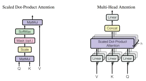
2.3.1 Scaled Dot-Product Attention

The input consists of queries and keys of dimension d_k, and values of dimension d_v. Com- pute the dot products of the query with all keys, divide each by√

d_k, and apply a softmax function to obtain the weights on the values.

In practice, a set of queries will be packed together into a matrix Q, and computation of the attention function will be simultaneous. The keys and values are also packed together into matrices K and V .

Attention(Q, K, V ) = sof tmax(QK^T

√d_k )V (2.11)

Figure 2.1: (left) Scaled Dot-Product Attention. (right) Multi-Head Attention consists of several attention layers running in parallel

(23)

2.3.2 Multi-Head Attention

A single attention function can represent one type of relation. If there are multiple attention functions, it can catch more relationships between entities. Linearly project the queries, keys and values h times with different, learned linear projections to d_k, d_k and d_v dimensions, respectively. Perform the attention function in parallel to each of the pro- jected versions of queries, keys, and values, yielding d_v-dimensional output values. These are concatenated and then projected again, resulting in the final values, as in Figure 2.1.

M ultiHead(Q, K, V ) = Concat(head₁, ..., head_h)W^O (2.12)

head_i = Attention(QW_i^Q, KW_i^K, V W_i^V)

The projections are parameter matrices W_i^Q ∈ R^d^model^×d^k, W_i^K ∈ R^d^model^×d^k, W_i^V ∈ R^d^model^×d^v and W^O ∈ R^hd^v^×d^model.

(24)

(25)

Chapter 3 Dataset

The Chapter describes the dataset used in this thesis.

3.1 Dataset Overview

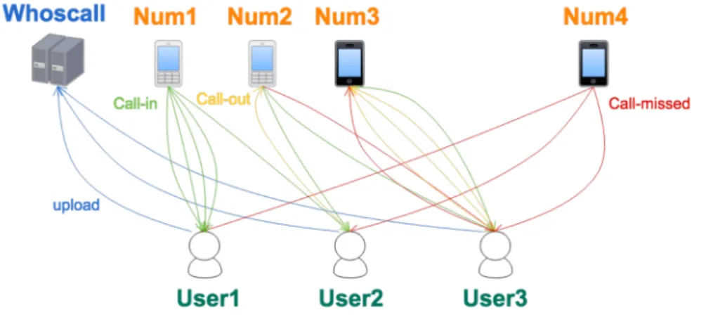
In our experiments, we use a dataset provided by Gogolook, which develops a smartphone application, Whoscall, on Android/iPhone for detecting whether an incoming call belongs to telemarketing, harassment, call centers, or frauds, based on known information such as yellow pages and Internet forums. The dataset was collected for a month in March 2018 from a group of voluntary users. The dataset was contributed by 2,221,711 voluntary app users, who collectively contributed a total of 16,634,311 remote phone numbers and 246,908,630 call records during the period shown in Table 3.1. With users’ consent, each call record comprises the time, user id, remote phone number, call duration, the ring tone type, whether the incoming call is in the contact book, the country code of the incoming call, whether the call is missed, etc.

In this dataset, each call record is an interaction between a user and a remote phone

March, 2018

# of call records 246,908,630

# of phone numbers 16,634,311

# of voluntary users 2,221,711 Table 3.1: Basic data statistics.

(26)

Phone Number

User Duration Direction Contact Starting Time

p1 u1 00:03:19 in yes 16:22:01

p2 u1 00:00:00 out yes 16:25:41

p1 u1 00:04:08 out yes 16:25:45

p2 u1 00:01:37 in yes 16:32:01

p3 u2 00:01:40 in yes 17:02:08

p4 u2 00:00:31 out yes 17:05:21

p4 u2 00:00:00 in yes 17:07:48

p5 u3 00:02:54 in no 17:09:01

p2 u3 00:17:35 in yes 17:12:18

p3 u2 00:03:14 out yes 18:07:08

p2 u2 00:00:00 out no 19:00:08

p2 u3 00:01:12 out yes 19:01:05

p5 u2 00:00:00 out yes 19:10:08

p1 u2 00:09:23 out no 19:12:32

p2 u2 00:00:57 in no 19:22:55

p2 u3 00:37:40 in yes 20:02:17

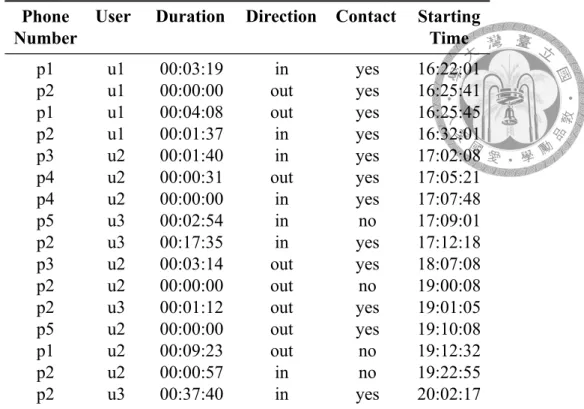
Table 3.2: An example of call logs.

number. For simplicity, we will just name them as user and phone number, respectively.

Each call has several attributes but we only use four of them as follows:

1. Duration: how long the call takes by second; zero indicates that the user did not answer the call

2. Direction: incoming call or outgoing call

3. Contact: whether the remote number is in the user’s contact book

4. Time: when the call is dialed

p1 p2 p1 p2 p3 p4 p4 p5 p2 p3 p2 p2 p5 p1 p2 p2

u1 u2 u3

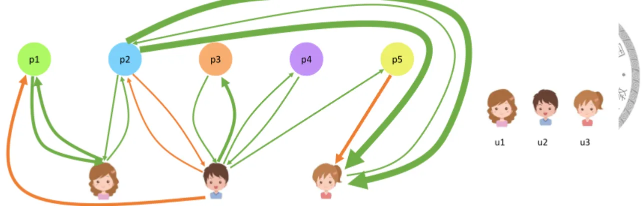
Figure 3.1: Visualized call logs

(27)

u1 u2 u3

p1 p2 p3 p4 p5

Figure 3.2: Bipartite graph of call logs

Note that call records in this dataset are incomplete. Not all call record related to a phone number is collected. We can only find records that interact with the user. Table 3.2 is an example of call logs, where each row in the call logs is a call between a user and a remote phone number. Figure 3.1 is the visualized version. The direction of the arrow indicates the direction of the call. The width of the arrow roughly indicates the duration of the call. The green arrow tells the phone number is in the user’s contact book.

One way to deal with the call logs is by using a graph. Figure 3.2 shows table 3.2 in a graph. As the edges connect the nodes altogether, it is not easy to get a reasonable subgraph. We can also line up call logs according to the phone number and form a call sequence. Figure 3.3 is the call sequence of p1 and p2. In this view of call logs, we can analysis a small part of call logs at a time.

There are user reports for phone number. After receiving a fraudulent call, an app user can report the phone number with a tag. The report also contains the report time so

p1 p1 p1 p2 p2 p2 p2 p2 p2 p2

u1 u2 u3

Figure 3.3: Call sequence of p1 and p2

(28)

Number Type # Numbers

Normal Number 16,609,081

Human-Annotated Fraud 23,434 Government-Reported Fraud 2,026

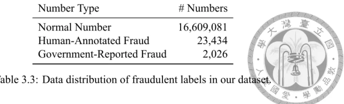
Table 3.3: Data distribution of fraudulent labels in our dataset.

we know when the phone number is reported. In the previous research [12], they notice the fraud label, harassment label, and telemarketing label are mixed and undistinguished.

Therefore, we use all these labels as fraud label. Another source of labels is provided by the National Police Agency (NPA), Ministry of the Interior. This kind of label is more sparse but accurate. Table 3.3 shows the distribution of normal phone numbers, human- annotated frauds, and government-reported frauds. Both labels are imbalanced, where the proportion of human-annotated fraud numbers in our dataset is 1/650.

(29)

Chapter 4 Related Work

There is a lot of research on fraud detection in telecommunications. America biggest telecommunication company AT&T had pointed out this problem [13]. Many approaches have been used in this area such as neural network and user profile based [14], LDA [15], Gaussian mixture model(GMM) [16].

4.1 Network Embedding

One of the approaches is to treat the interaction between users and phone numbers as a network. In Figure 4.1, each user or phone is a node in the bipartite graph. Each call interaction between the user and the phone number is represented by an edge. There are many network embedding methods that can construct an embedding for each node. Then

Figure 4.1: A bipartite phone call graph

(30)

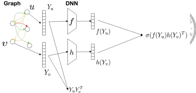
Figure 4.2: Network embedding for phone call graph

we can learn a classifier to detect fraud from phone numbers based on their embedding.

Lee [12] utilize this method on fraud detection. Figure 4.2 is his model. Similar to [17], he uses two projection matrix to project the two vectors Yu and Yv from a call between u and v. To maximize the graph likelihood, he makes the cosine similarity of the two outputs close to a co-occurrence matrix. The two different projection matrix will thus consider the direction attribute. To generate the co-occurrence matrix, they use low-rank approximation [18] instead of simulating random walk [19, 20], and weight each node with its call frequency. Finally, they minimize the root mean square error between the call duration and the cosine similarity of the two node embedding.

Although the network embedding contains rich information about the graph, only the seen entity has an embedding. We would have zero knowledge about a new phone number.

Adding new nodes and edges is a solution, but the network embedding will need fine tuning or even training from scratch. This makes it hard to use in real time analysis.

4.2 Real Time Analysis

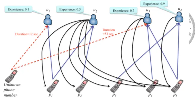
Tseng et al. [21] uses Weighted Hyperlink-Induced Topic Search algorithm to learn a trust value for each phone number and an experience value for each user. In Figure 4.3, user u₁ to u4 have learned experience values, representing their ability to detect fraud and hang

(31)

Figure 4.3: FrauDetector

up. Based on the learned trust value, experience value, they can calculate the trust value of the unknown phone number according to the statistic of the calls. With a proper threshold set in the light of the learned trust value from p₁ to p₅, they will know how likely the unknown phone number is a fraud. However, they only use aggregated features such as total duration a phone number and call frequency of a phone number. Their model loses the order of call and many details in the interaction between users and phone numbers.

4.3 Summary

Network embedding is a great way to capture complicate relations in a graph. Phone numbers with similar characteristics will be close in the embedding space. With network embedding, Lee [12] can train a very good classifier to detect fraud. However, he can only detect on old numbers appearing in training time. On the other hand, Tseng et al. [21] can detect in a real time scenario. They use an EM-like training procedure to learn the experience value and the trust value. With the two kinds of related value, they can approximate the trust value for unknown phone numbers. Nevertheless, they only use aggregated call graph instead of raw call logs. This will lose some important information. Another problem is the metric they used. AUC on ROC isn’t suitable for imbalanced classification

(32)

problems. One can easily create a classifier with a high value in AUC on ROC but have poor performance. In contrast, our model uses raw call logs directly to recognize the behavior of the phone number and is able to apply on new unknown phone number.

(33)

Chapter 5 Problem Formulation

5.1 Goal

We want not only to recognize the fraudulent phone number but also to detect the future fraudulent phone number. Therefore, given the training data up to now, we would like to detect well in the future.

5.2 Input

For each phone number, there is a sequence of call records related to it. Each call record contains five features.

1. User ID: whom the phone number interacts with.

2. Duration: how long the call takes by second; zero indicates that one of them did not answer the call

3. Direction: incoming call or outgoing call

4. Contact: whether the phone number is in the user’s contact book 5. Time: when the call is dialed

(34)

5.3 Output

Each phone number has a label indicating whether it is fraud, but we want the fraudulent probability of each phone number instead of binary output. This allows comparing the ability of two models. It is also more useful for real application where different trade-off could be considered.

5.4 Evaluation metrics

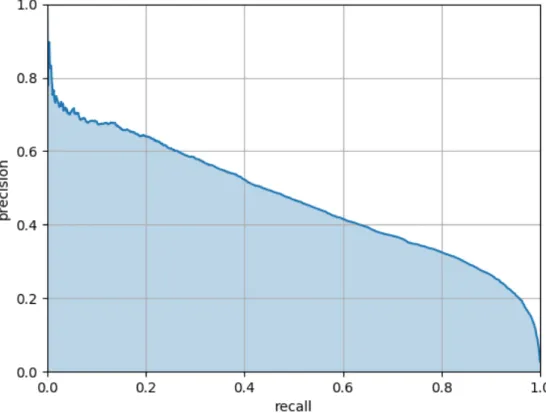
This is an imbalanced binary classification problem. To consider both precision and recall, we use the average precision, the precision averaged across all values of recall between 0 and 1. This value will be similar to the Area Under Curve(AUC) of Precision-Recall Curve(PRC), which is more appropriate then AUC of Receiver Operator Characteris- tic(ROC) [22]. Figure 5.1 shows a precision-recall curve, and the blue area is average precision.

Figure 5.1: Precision-recall curve

(35)

To draw the precision-recall curve, Sort all the probability first. For each threshold of probability, draw a dot by corresponded precision and recall. Connect the dots to form the precision-recall curve. In particular, we calculate the precision at the first recall. Then, for every 0.1% of recall, a precision is calculated. There will be 1001 precision values.

We calculate the trapezoidal interpolation of the precision as average precision.

The random guess baseline of this metric is the percentage of the positive label. If only 1% of the sample is positive, the average precision of the random baseline will be 1%. That is, having 1% of precision for all recall.

(36)

(37)

Chapter 6 Model

6.1 Overview

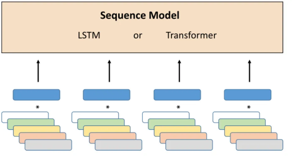
The task is to learn real-time call representations for fraudulent call detection and this thesis proposes a novel sequence-based call behavior modeling framework, where the calls between a particular remote number are lined up to form a sequence, named “remote sequence”. Each call in the sequence has associated attributes, including user ID, duration, direction, whether the remote phone number is in the user’s contact books, and time. Mo- tivated by the recent advances of pre-trained informative models such as ELMo [3] and BERT [4], the proposed approach first learns rich representations from sequences and then predict whether each call is fraudulent or not based on the learned number embeddings.

In our proposed model, there are two phases: 1) call behavior modeling and 2) fraud detection. As illustrated in Figure 6.1, in the call behavior modeling phase, there are two modules:

• Latent cross for feature fusion: Latent Cross [23] is an elegant way to fuse the main feature with several auxiliary features.

• Sequence modeling for capturing real-time, dynamic features: After passing the latent cross module, we have a latent representation for each call, still, line up in a sequence. To make our model consider the order of calls, we use LSTM [24]

or Transformer [9] as our sequence models considering their superior capability of

(38)

* * * *

Sequence Model

LSTM or Transformer

Figure 6.1: Illustration of the call behavior modeling phase.

modeling sequential information.

The concept is inspired by the work about recurrent recommendation systems proposed by Beutel et al. [23]. Their model first fuses several features and generate a representation for each time step. Then, use the representation to recommend the next video. Although our task is not to recommend or predict the next call, the ability to utilize several features and generate dynamic representation match our needs. Therefore, we use a similar architecture to build our model. We think that a model that can predict the remote sequence well must contain rich information for the call behaviors. In the call behavior modeling phase, the sequence model is trained to predict the next call given the previous call sequence in order to model the call behaviors and produce the corresponding number representations.

𝑟_𝑡−1^𝑙−1 𝑟𝑡𝑙−1 𝑟_𝑡+1^𝑙−1

𝑟_𝑡−1^𝑙 𝑟_𝑡^𝑙 𝑟_𝑡+1^𝑙

𝑟_𝑡−1^𝑙+1 𝑟𝑡𝑙+1 𝑟_𝑡+1^𝑙+1

Aggregated embedding

Fraud detector A simple classifier

Figure 6.2: Illustration of the fraud detection phase.

(39)

After pre-training the model to capture the call behaviors, there are two modules in the fraud detection phase, as illustrated in Figure 6.2:

• Embedding aggregation for leveraging the learned number representations: The learned number representations have two dimensions for aggregating features, time and layer; within one dimension, there are also several ways to combine feature embeddings such as concatenation and pooling.

• Fraud detection for predicting whether the call is fraudulent or not: After aggregating the learned number representations, a classifier uses a fully connected layer and an output layer to determine the probability of the call is fraudulent.

Four components, 1) a latent cross model tries to aggregate multimodal features in call behaviors, 2) A sequence model focuses on learning the corresponding representations for call sequences, 3) an aggregation module combines the embeddings to represent each number, and 4) a fraud detector utilizes the representations to predict if the incoming call is normal or fraud, are detailed below.

6.2 Feature Fusion

With various features for each call, a remote sequence is a sequence of user numbers with the associated attributes. Therefore, we treat user numbers as our main feature and other features as auxiliary features. For the primary feature, user number, each number has its own embedding. The auxiliary features that are continuous are quantized into discrete features, where each level has the feature embedding with the same dimension as user embedding.

Beutel et al. [23] proposed the latent cross technique, where multiple latent representations can be fused to form a rich embedding. When combining several latent representations, the most common way is concatenation. We can concatenate several feature vectors, forming a long vector, and pass it to the next layer. They claimed that neural networks are inefficient in modeling the interactions between concatenated input features, and proposed an alternative method to fuse input features. Taking one main feature and

(40)

Level 1 2 3 4 5

Range 0 1∼ 2 3∼ 6 7∼ 14 15∼ 30

Level 6 7 8 9 10

Range 31∼ 62 63 ∼ 126 127 ∼ 254 255 ∼ 510 510∼ Table 6.1: Call duration level

two auxiliary features as example, let h^{(τ )}be the primary feature vector and wt, wdbe two context feature vectors. ˆh^{(τ )} is the fused vector:

ˆh^{(τ )}= h^{(τ )}∗ (1 + wt+ w_d) (6.1)

We perform element-wise product between context features and primary features to form the fused vector. The context feature vectors are initialized by a zero-mean Gaussian. This can be interpreted as a mask or the attention mechanism.

In our model, we use four context features, including call duration, call direction, whether the remote number is in contact book, and the time of the call as described in Chapter 5. We split call duration into 10 levels by the length, where the first level indicates that the phone rings but no one answers. The second level is the call with 1 to 2 seconds long. Table 6.1 details the duration range for each level. In terms of call direction, a boolean feature is adopted: 1) the user dials to a remote number or 2) a remote number dials to the user. Whether the remote number is in the user’s contact book is a boolean feature. We split a day into 12 time slots to create the time features.

The output of latent cross modules is a sequence of embedding vectors. Each output vector represents a call embedding that fuses multiple features.

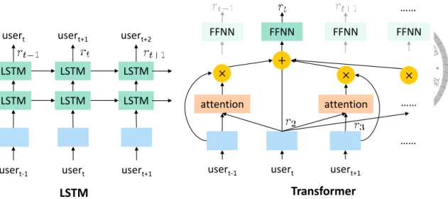
6.3 Sequence Modeling

With the rich embeddings for calls as the input, to extract useful information from sequences, two models are adopted. LSTM and Transformer are good at modeling sequential data illustrated in Figure 6.3. The hidden size of LSTM and Transformer are the same as input embedding size for simplicity. Both LSTM and Transformer have dynamic lengths,

(41)

FFNN

attention

user_t-1

FFNN

user_t

FFNN

attention

user_t+1 +

× ×

FFNN

LSTM × LSTM

user_t-1

LSTM LSTM

user_t

LSTM LSTM

user_t+1

LSTM Transformer

user_t user_t+1 user_t+2

……

Figure 6.3: Illustration of sequence models applied in the model.

allowing our model to take any length of remote sequences as the input.

For the LSTM model, we use 2 LSTM layers as shown in the figure. For the Trans- former model, we use 1 Transformer block. The input is first added with a positional encoding. The sub-layers are a masked multi-head self-attention and a feed-forward network. We apply masking to attention because while pre-training, the model should not see the next label. The feedforward network consists of two linear transformations with a ReLU activation in between.

F F N N (x) = max(0, x· W1+ b₁)· W2+ b₂, (6.2)

where F F N N (x) is the representation corresponding to the specific input in the sequence illustrated in Figure 6.3.

In this task, our goal is to detect fraudulent calls. However, the label size is relatively sparse compared to the data size. To enable learning without the labels for sequences, pre-training the feature extractor with a prediction task can make the feature extractor know the underlying structure of sequences. Motivated by the recent advances achieved by ELMo [3] and BERT [4], where they treat the next word as the target to enable unsu- pervised training, and the pre-trained models carry informative cues for various language understanding tasks because the linguistic knowledge is modeled by the pre-trained model.

In our task, we set the prediction target each time step is the user id and direction at the

(42)

next time step. The goal is to capture the call behaviors for a number in a dynamic manner.

To train the next call predictor, we use softmax cross entropy loss. This needs to perform a linear transform on the outputs of the last LSTM layer. We allow the linear transform to share weights with user embedding vector. U is the whole user embedding matrix. w, b are two transform matrices. h_i is the learned representation at t-step. The next user id u_t+1is formulated as

W = w∗ U, (6.3)

B = b∗ U, (6.4)

u_t+1 = arg max(h_i∗ W + B). (6.5)

There are a few reasons to use share weights. First, the prediction target domain is the same as the input user domain. There is no reason to learn one thing twice. For example, if the model has learned the embedding of user id 3, it should know when to predict the next user id is 3. Second, the main goal of the prediction task is to allow the sequence model to learn from sequences. Here, the linear transformation is not used for the following modules, because the call embeddings learned by the sequence model come from the hidden layers instead of the final prediction layer.

6.4 Embedding Aggregation

With the representations learned by the sequence model, our goal is to build a classifier to tell whether the remote number is a fraud. To enable real-time inference, there is a tradeoff between the number of time steps used in the classifier and the achieved performance, because the output representation of each time step contains rich information. In the above sequence models, the goal is to learn the representations that can reflect the information from the whole sequence. The former time step depends on less input of sequence. If the classifier only uses the last time step, the model could be used for any length of a remote sequence but its performance may not be good. If the classifier uses the last 20 time steps, it has more information about the sequence but can only be used on those sequences which

(43)

longer than 20. On the other hand, it has less training data since it can only be trained with sequences which longer than 20. When the performance is compatible, we would like to use the model which uses fewer time steps for its ability to detect on a shorter sequence, allowing fast detection. We can identify the fraud right after they show up.

Figure 6.4 shows the two dimensions needed to aggregate. This is a two layer LSTM model with three calls as input. Each square is a vector. In the left part, we want to aggregate the output of feature extractor over time steps. There are two kinds of classifiers, whether they use the fixed length of feature extractor outputs or not. Using a dynamic length of feature extractor outputs can give us the flexibility to predict both long sequences and short sequences. To build a dynamic length classifier, we can use a pooling on several time steps. We use mean-pooling and max-pooling. To build a fixed length classifier, we first decide how many time steps to take. We have two ways to aggregate over time step, concatenation, weighted sum.

Though mean-pooling and max-pooling have fully dynamic input length, we still set a minimum input length for them. We think a meaningful judgment should have suffi- cient information. Making detection with an extreme short sequence such as only one call doesn’t make sense. Let minL be the minimum length of the detect model. Concatena- tion model will concatenate over the last minL time steps. Weighting model will get a weighted sum over the last minL time steps. The mean-pooling model will do a mean- pooling over the last minL time steps. Max-pooling model will do a max-pooling over the last minL time steps.

call call call call call call

Figure 6.4: (left) Aggregation over time steps. (right) Aggregation over layers.

(44)

In the right part of Figure 6.4, we also aggregate the output of feature extractor over layers. For a two layers LSTM feature extractor, there are three layers, the output of latent cross modules and the output of two LSTM layers. For Transformer feature extractor, there are always two layers, the output of latent cross modules and the output of Transformer.

L_iis the i-th step of latent cross. h^l_iis the output of i-th step of l-th LSTM layer. The basic way is only to use the topmost layer h²_i. Another typical way is concatenating all layers [h²_i; h¹_i; L_i]. The last one is doing a weighted sum over the layers with trainable weights h²_i ∗ w1+ h¹_i ∗ w2+ Li∗ w3.

6.5 Fraud Detection

After two-dimensional aggregations, we obtain a flat latent vector for representing the real-time number behavior. We use a hidden layer with 256 neurons and an output layer with a single neuron to build the detector. We use sigmoid cross entropy loss for detector training.

6.6 Training and Inference

In our training procedure, we apply two-phase training. First pre-train the model without the classifier. The training target is to predict the next user and the next direction, just like training a recommender or language model. After pre-train, we train the classifier with detection loss.

In the inference stage, to detect whether a new remote phone number is fraud or not, we just line up those new calls into a remote sequence and apply our detect model. Then the detector can perform in real-time once we collect at least k calls in the sequence.

This is a binary classification task on the extreme imbalance dataset. A detection model should give each remote sequence a probability of fraud. We can set a threshold depending on our needs. Different thresholds give different precisions and recalls. The performance of precision and recall is a trade-off in real applications.

(45)

Chapter 7 Experiment

To evaluate the performance of the proposed approach, a set of experiments are conducted.

7.1 Setup

The experiments are conducted on the collected call behaviors built on the dataset in chapter 3. The dataset includes calls in March 2018, along with human annotation and Gov- ernment report. We take the first 20 days as training data and the rest as testing data. All calls and labels in the first 20 days are available in training. Testing data only contains calls happened in the last 11 days. Note that some remote phone numbers may have calls in the first 20 days and the last 11 days. If such calls are enough to construct a remote sequence in training data as well as testing data, there are some remote sequences generated by the same remote number across training data and testing data. Half of the testing data serves as our validation set, and another half is real testing. The validation set and the test set are interleaved so they have similar features in all aspects we know. For the fraud detection task, a remote sequence has a positive fraud label if there is any report on the remote number.

As our model uses number embeddings to classify the remote number, a well-trained embedding is important. The calls with users who do not exist in training data or only exist in sequence shorter than 20 are removed. The remaining sequences contain only useful calls. Removing some calls from the sequence would not affect the meaning of

(46)

the sequence since our remote sequence is not a full history for the remote phone number. Remove some calls from sequence would not destroy the information hidden in the sequence.

We use the first 7 days of data for testing. If the selected interval is small, we can claim that a good model is able to make good predictions in real-time. Each remote number has an associated remote sequence in testing data. For sequences with the length over 20, we reserve the last 20 calls and drop the rest.

There are sequences generated from the same remote phone number in training data and testing data. These sequences in testing data should be easier cause the model has seen the behavior of the remote number. Although our target is overall average precision, We monitor the average precision among this kind of sequence to know more about the characteristic of the model. We also monitor the average precision among those only new in testing data. Some models can use a shorter sequence so they can utilize the training data more. This also let them learn from more remote number than those model which use long sequences.

All feature embeddings for latent cross are 256 dimensions. The multi-head self- attention used in Transformer has 8 heads. The dimensionality of the input and output in the sequence model is 256, and the inner-layer has 1024 dimensions.

7.2 Result

There are three recipes for our two-phase training.

• No pre-training: we directly train the detector with both phases.

• Pre-training and fine-tuning: we pre-train the sequence models for learning number embeddings, and fine-tune the weights of embeddings when training the classifier.

• Pre-training and classifier training: we pre-train the sequence models for learning number embeddings, and fix the weights of embeddings when training the classifier.

In table 7.1, we can see the sequence model is good at modeling sequential information by comparing the No Pre-Training with baselines. Furthermore, the pre-training with the

(47)

LSTM Transformer

Baseline Random 2.73

No Sequence model 32.42

No-order Sequence model X 38.29

Proposed No Pre-Training 37.74 39.49

Pre-Train & Fine-Tune 39.81 44.56 Pre-Train & Classifier 48.52 45.19

Table 7.1: Average precision of proposed models. The classifier concatenates over layers and operates mean-pooling over time steps. (%)

prediction task did learn a more powerful sequence model. By observing the training curve of Pre-train & Fine-Tune, we discover that the model does the best at the first epoch then the performance went down. We can say the classification loss isn’t a good training target for call behavior modeling.

7.3 Effectiveness of Features

In [21], they show the importance of call duration and frequency. We want to find what feature is more useful in the latent cross module. To know the importance of each auxiliary feature, we replace feature to see the influence of average precision. There are two options of replacement, zero vector or random vector. The design of latent cross treats each auxiliary feature as a mask vector or an attention vector, so it is reasonable to hide the information with zero vector. On the other hand, replace with zero vector will change the output variance from the latent cross module. Zero means simply remove the target feature. Random means replace each target feature with a newly initialized vector. Scale means zero out the target feature and multiplies 4/3 to the other three features. Table 7.2

Zero Rand. Scale Overall Rel. Diff.

Full 48.52

- Duration 48.72 47.29 49.19 48.40 -1.16%

- Direction 40.64 37.60 40.21 39.48 -19.38%

- Contact 43.85 42.25 42.41 42.84 -12.52%

- Timeslot 49.51 48.71 49.04 49.09 +0.25%

Table 7.2: Average precision for ablation study of auxiliary features. The classifier concatenates over layers and operates mean-pooling over time steps. (%)

(48)

Over Layer Over Time LSTM Transformer concatenate concatenate 42.74% 42.84%

concatenate weighting 43.96% 43.82%

concatenate max-pooling 48.02% 46.22%

concatenate mean-pooling 48.52% 45.19%

top-layer mean-pooling 40.94% 42.33%

weighting mean-pooling 41.49% 43.33%

weighting concatenate 43.15% 41.46%

Table 7.3: Average precision of different aggregations.

shows the ablation result on LSTM.

7.4 Comparison of Aggregation Methods

There are several ways to aggregate rich information from the sequential model. Methods like concatenation and pooling are non-parametric, making the training easier. Weighted sum over latent representation has been used in many embedding methods [3]. Aggrega- tion over layer and aggregation over time step could use a weighted sum method.

Table 7.3 show concatenating over layer is more useful than the other two ways. The LSTM can’t pass through all information and concatenating over layer will allow the later module to see full information. Pooling over time step is more useful than other methods.

7.5 Embedding Visualization

We randomly select remote sequences from both the fraud number and the normal number and visualize the aggregated representation of the classifier with non-trainable aggregation method. These part of model can be trained with only un-annotated sequence and extract meaningful representation.

The PCA analysis shows the importance of pre-train prediction task. We take the model after pre-train, which means the model hasn’t seen any fraud label, and visualize the aggregated vector. The aggregated vector is the input of the classifier. In PCA analysis, the two most important eigenvector from the aggregated vector is used to plot the Figure 7.1.

The LSTM model and Transformer model aggregate with concatenating over layer and

(49)

Figure 7.1: PCA visualization of aggregated representation. Fraud and normal ratio is 1:4

Figure 7.2: PCA visualization of aggregated representation with name. The red dots are fraud and the words are their name labels.

mean-pooling over time step. The red dots belong to fraud remote number and the blue dots belong to normal remote number. It is clear that fraud and normal are separated horizontally. The x-axis dimension has the biggest variance in PCA analysis.

7.6 Tradeoff Between Performance and Time Lag

To handle the time lag problem, we want to perform detection on a remote number as soon as possible. However, fast detection means detecting with fewer calls, which harms the detection performance. Table 7.4 shows the tradeoff between dataset 10 and dataset

(50)

min length dataset 20 dataset 10

Random Baseline 2.73 1.15

No Sequence Baseline 32.42 30.54

LSTM 20 48.52 39.30

10 49.11 41.23

Transformer 20 45.19 38.05

10 24.92 40.83

Table 7.4: All concatenate over layers and operates mean-pooling over time steps. Aver- age precision with dataset 20 and dataset 10.

20. Dataset 20 contains remote sequences longer than 20. Dataset 10 contains remote sequences longer than 10. Sequences longer than 20 is truncated to length 20, so the dataset 20 is included in the dataset 10, so dataset 10 much harder than dataset 20.

(51)

Chapter 8 Conclusion and Future Work

With a pre-train prediction task, our model can extract hidden information from large unannotated data. The visualization of latent representation expresses a clear difference between the fraudulent number and the normal number. Our experiment shows this kind of hidden information can enormously improve the precision of fraud detection problems.

A potential future research direction will be tracking multi phone numbers. As our model look a single phone number at a time, we may miss detecting the fraud consist of multiple phone numbers.

(52)

(53)

Bibliography

[1] J. Burez and D. Van den Poel, “Handling class imbalance in customer churn predic- tion,” Expert Systems with Applications, vol. 36, no. 3, pp. 4626–4636, 2009.

[2] C. Phua, D. Alahakoon, and V. Lee, “Minority report in fraud detection: classifica- tion of skewed data,” Acm sigkdd explorations newsletter, vol. 6, no. 1, pp. 50–59, 2004.

[3] M. Peters, M. Neumann, M. Iyyer, M. Gardner, C. Clark, K. Lee, and L. Zettlemoyer,

“Deep contextualized word representations,” in Proceedings of the 2018 Conference of the North American Chapter of the Association for Computational Linguistics:

Human Language Technologies, Volume 1 (Long Papers), pp. 2227–2237, 2018.

[4] J. Devlin, M.-W. Chang, K. Lee, and K. Toutanova, “BERT: Pre-training of deep bidirectional transformers for language understanding,” in Proceedings of the 2019 Conference of the North American Chapter of the Association for Computational Linguistics: Human Language Technologies, Volume 1 (Long Papers), 2019.

[5] J. R. Firth, “A synopsis of linguistic theory 1930-55.,” in Studies in Linguistic Anal- ysis (special volume of the Philological Society), vol. 1952-59, pp. 1–32, Oxford:

The Philological Society, 1957.

[6] T. Mikolov, K. Chen, G. Corrado, and J. Dean, “Efficient estimation of word repre- sentations in vector space,” Proceedings of Workshop at ICLR, 2013.

[7] J. L. Elman, “Finding structure in time,” Cognitive science, vol. 14, no. 2, pp. 179–

211, 1990.

(54)

[8] S. Hochreiter and J. Schmidhuber, “Long short-term memory,” Neural computation, vol. 9, no. 8, pp. 1735–1780, 1997.

[9] A. Vaswani, N. Shazeer, N. Parmar, J. Uszkoreit, L. Jones, A. N. Gomez, Ł. Kaiser, and I. Polosukhin, “Attention is all you need,” in Advances in neural information processing systems, pp. 5998–6008, 2017.

[10] K. He, X. Zhang, S. Ren, and J. Sun, “Deep residual learning for image recognition,”

in Proceedings of the IEEE conference on computer vision and pattern recognition, pp. 770–778, 2016.

[11] J. L. Ba, J. R. Kiros, and G. E. Hinton, “Layer normalization,” arXiv preprint arXiv:1607.06450, 2016.

[12] C.-H. Lee, “A network embedding on phone call graph,” Master’s thesis, National Taiwan University, 2018.

[13] R. A. Becker, C. Volinsky, and A. R. Wilks, “Fraud detection in telecommunications:

History and lessons learned,” Technometrics, vol. 52, no. 1, pp. 20–33, 2010.

[14] M. Weatherford, “Mining for fraud,” IEEE Intelligent Systems, vol. 17, no. 4, pp. 4–

6, 2002.

[15] D. Olszewski, “A probabilistic approach to fraud detection in telecommunications,”

Knowledge-Based Systems, vol. 26, pp. 246–258, 2012.

[16] M. I. M. Yusoff, I. Mohamed, and M. R. A. Bakar, “Fraud detection in telecommuni- cation industry using gaussian mixed model,” in 2013 International Conference on Research and Innovation in Information Systems (ICRIIS), pp. 27–32, IEEE, 2013.

[17] S. Abu-El-Haija, B. Perozzi, and R. Al-Rfou, “Learning edge representations via low-rank asymmetric projections,” in Proceedings of the 2017 ACM on Conference on Information and Knowledge Management, pp. 1787–1796, ACM, 2017.

[18] S. Cao, W. Lu, and Q. Xu, “Deep neural networks for learning graph representa- tions,” in Thirtieth AAAI Conference on Artificial Intelligence, 2016.

(55)

[19] B. Perozzi, R. Al-Rfou, and S. Skiena, “Deepwalk: Online learning of social repre- sentations,” in Proceedings of the 20th ACM SIGKDD international conference on Knowledge discovery and data mining, pp. 701–710, ACM, 2014.

[20] A. Grover and J. Leskovec, “node2vec: Scalable feature learning for networks,”

in Proceedings of the 22nd ACM SIGKDD international conference on Knowledge discovery and data mining, pp. 855–864, ACM, 2016.

[21] V. S. Tseng, J.-C. Ying, C.-W. Huang, Y. Kao, and K.-T. Chen, “Fraudetector: A graph-mining-based framework for fraudulent phone call detection,” in Proceedings of the 21th ACM SIGKDD International Conference on Knowledge Discovery and Data Mining, pp. 2157–2166, ACM, 2015.

[22] T. Saito and M. Rehmsmeier, “The precision-recall plot is more informative than the roc plot when evaluating binary classifiers on imbalanced datasets,” PloS one, vol. 10, no. 3, p. e0118432, 2015.

[23] A. Beutel, P. Covington, S. Jain, C. Xu, J. Li, V. Gatto, and E. H. Chi, “Latent cross:

Making use of context in recurrent recommender systems,” in Proceedings of the Eleventh ACM International Conference on Web Search and Data Mining, pp. 46–

54, ACM, 2018.

[24] F. A. Gers, J. Schmidhuber, and F. Cummins, “Learning to forget: Continual pre- diction with lstm,” in Proceedings of the 1999 Ninth International Conference on Artificial Neural Networks ICANN 99. (Conf. Publ. No. 470), IET, 1999.