Unraveling Impact of Critical Sensing Range on Mobile Camera Sensor Networks
Xiaoying Gan1,3, Zesen Zhang1, Luoyi Fu2, Xudong Wu2, Xinbing Wang1,2
1,2Dept. of{Electronic Engineering, Computer Science}, Shanghai Jiao Tong University, China.
3National Mobile Communications Research Laboratory, Southeast University F
Abstract—In camera sensor networks (CSNs), full view coverage, meaning that any direction of any point in the operational region is covered by at least one camera sensor, plays a significant role in object identification. While prior work is dedicated to static CSNs for the seek of critical condition to achieve full view coverage, such performance still remains unknown in mobile CSNs. In this paper we take the initiative to address this issue, where a centralized parameter, i.e., equivalent sensing radius (ESR), is defined to unravel the critical requirement for asymptotic full view coverage in mobile heterogeneous CSNs in the sense that camera sensors of different sensing capabilities are moving around in target area. Specifically, we derive ESR under three different mobilities, i.e., 1-dimensional and 2-dimensional random walks and random rotating model, and then explore respectively the corresponding critical conditions to achieve almost surely coverage1. The static network is introduced as a baseline in order to gain a clear understanding of how mobility affects coverage performance differently. Interestingly, we find that both 1 dimensional and 2 dimensional random walks exhibit a smaller ESR than static one whereas ESR is even larger in random rotating mobility than that in static CSNs. Moreover, the almost surely coverage is found to be around 1.225 times of the critical condition to achieve coverage with high probability2, and therefore turns out to be a stronger result compared to the traditional coverage with high probability.
We then turn to the impact of various mobility patterns on sensing energy consumption, a metric that is closely related to ESR, and show that it can be decreased by random walks under certain delay tolerance.
The relationship between ESR and percentage of full view coverage is also discussed and the results unify those under homogeneous CSNs.
1 I
NTRODUCTIONCoverage, as a crucial performance metric, is commonly used in Wireless Sensor Networks (WSNs) in measure- ment of how well a target field is monitored by sensors.
Intuitively, a better guarantee of coverage can lead to higher network controllability, and therefore manifests its importance in a wide range of control-aware appli- cations such as security surveillance, traffic control, en- vironmental monitoring, intrusion detection, industrial
The early version of this paper is appeared in the Proceedings of IEEE INFOCOM 2014 [27].
1. Let Anbe a countable collection of sets, and lim supn→∞An=
∩∞
n=1
∪
m≥nAm, which means that for every element in the lim sup, for every N , there exists an An with n ≥ N that has the element.
For event An, ifP(lim supn→∞An) = 1, we say the event An will almost surely happen or happen infinitely often. Let lim infn→∞An=
∪∞
n=1
∩
m≥nAm, which means that for any element in the lim inf, there is an N such that the element is in every Anfor any n≥ N. For event An, ifP(lim infn→∞An) = 1, we say the event Anwill happen eventually.
2. If event An satisfies limn→∞P (An) = 1, then event An will happen with high probability.
process control [1] and etc. As a kind of derivative of WSNs, Camera Sensor Networks (CSNs) have recently attracted an increasing amount of attention due to the significant ability of visual information collection, and consequently can provide more comprehensive and ac- curate information about real-time situation. Different from traditional sensors that possess omnidirectional sensing ability, a camera sensor is only capable of sensing within a certain angle of view, beyond which it fails to capture any information.
Such phenomenon can be briefly attributed to the viewing direction, which, as a property that exclusively belongs to camera sensors, distinguishes the coverage issue of CSNs from the one that has been intensively studied in conventional WSNs [2]- [13]. The main reason is that the model suggested by those works characterizes coverage through simply assuming that an object is con- sidered to be covered if it is within the sensor’s sensing range, which is usually supposed as a disk. However, when it comes to a CSN, such simplification falls short of well reflecting the features of camera sensors in the sense that the model fails to embody viewing direction. To solve this, Wang et al. [14] took a pioneer step ahead by proposing a novel concept called full view coverage in judgement of coverage performance in CSNs. An object is said to be full view covered if its viewed direction is always sufficiently close to its facing direction, regardless of wherever it actually faces. The advantage of full view coverage lies in incorporating the object recognition [15], and meanwhile guarantees that every perspective of an object at any point is under the view of some camera sensor if the target area is full-view covered.
A key step to construct a full-view covered CSN is to find out under which conditions such full view coverage can be achieved. Nevertheless, in contrast to the huge efforts made in traditional WSNs, the issue of coverage in CSNs still remains underexplored. With their proposed coverage metric as stated above, Wang et al.
[14] considered two types of deployment, i.e., random and uniform deployment and the lattice based one in CSNs, and provided a sufficient condition for full view coverage in the former one as well as a critical (i.e.
both necessary and sufficient) condition under the latter.
Following that, Wu et al. [16] introduced heterogeneity into the CSN, where they also analyzed the necessary
and sufficient conditions to achieve full view coverage, respectively. Another line of existing works are con- cerned with full view barrier coverage in CSNs [17] [18].
All these works are commonly based on static net- works for the seek of coverage condition. With recent development in electronic technology and image sensors, it is possible to deploy mobile CSNs with camera sensors moving in the area of interest and takeing pictures or live videos simultaneously. The ability of mobility greatly expands CSN’s application range [19], while the use of mobile camera sensors also brings about benefit of enlarging the monitored area as mobile cameras are able to move toward any corner of the area of interest.
Specifically, as demonstrated by Liu et al. [20] and Saipulla et al. [21], mobility can lead to improvement of barrier coverage performance since it may reduce the detection time of intruders. However, a question remains unknown: how could mobility potentially enhance coverage in CSNs? And to what extent?
To address this issue, we present a first look into cover- age problem in mobile CSNs. Leveraging the conception of full view coverage in [14], we focus on the critical coverage condition in three different mobility models, i.e, 1-dimensional and 2-dimensional random walks as well as random rotating mobility. Moreover, we use static network as a baseline to get a clear understanding of the benefit brought by mobility. For the sake of tractabil- ity, here we consider asymptotic coverage in the sense that the total number of cameras approaches to infinity.
Specifically we focus on a metric Equivalent Sensing Range (ESR), which, as pointed out by previous study [13], plays a vital role in determining the full coverage of the whole sensor network, regardless of the total number of sensors or the sensing radius of a single senor under random mobility patterns, and is thus a much easier and more general way to operate coverage control. However, unlike the sensing range of traditional sensors, here it relies heavily on several key factors such as the angle of view (or in other words, viewing direction), sensing radius, deployment density of camera sensors, and etc.
To quantify this element, we introduce the conception of Equivalent Sensing Range (ESR), of which rigorous definition will be provided in Section II.
Here it is worthwhile noting that in our definition of ESR, we also take into consideration the heterogeneity of camera sensors. The introduction of heterogeneity co- incides well with the fact that camera sensors may come from different manufacturers and thus have different sensing parameters, or the sensing capability of cameras will decline with the elapse of time or vary under different obstruction of terrains. Specifically, we deal with camera heterogeneity through dividing them into different groups according to their sensing parameters as is similarly conducted in [22] [23]. Then we define in all the four scenarios the corresponding ESRs, which incorporate the combined effects of viewing direction, camera heterogeneity and mobility patterns. Based on
those, we derive critical ESRs under four mobility cases3 with uniform sensor deployment4. The merit of critical ESR lies in facilitating the evaluation of the overhead for a CSN to achieve full view coverage, and both the advantages and drawbacks incurred by mobility are disclosed through the results.
However, there are several significant works that seem to be similar with our work. The work [29] is one of them. We have to admit that our work does share some similarity with Kumar’s literature in terms of the technical structure. Despite of that, there still exist may differences between the two works.First of all, our work assumes that the sensor just have partial view, which is much closer to the reality. And the Φ considered is not simply a constant, as we shown in Section 2.1 that “All sensors in group Gyhave identical sensing radius ryand angle Φy,but either ry̸= rzor Φy̸= Φzwill hold if y̸= z.
So our Φ will change as n varies. In addition, though our analysis looks similar to that in Kumar’s work in terms of the structure, our main contribution is on the CRITICAL ESR, which is
√3
2 ESR in the literature. With the introduction of critical ESR, we are able to find the tighter condition than that discovered in Kumar’s work.
Last but not least, our work addresses the first of several future directions that Kumar pointed out in Section 4 in his work. Overall, all those factors suffice to differ our work from Kumar’s.
Our main contributions are highlighted as follows.
1. We provide the critical conditions (critical ESR) of full view coverage or coverage with high probability under four different mobile situations. Specifically, our results disclose that the critical ESRs derived under random walks can be reduced by approximately an order of Θ
(√log n+log log n nθ
)
, where n and θ respectively represent the number of camera sensors and viewing angle, compared to that under static CSNs, whereas the random rotating mobility leads to a critical ESR twice than that of static CSNs.
2. We also derive the critical condition to achieve almost surely coverage, which is shown to be approxi- mately 1.225 times of that to achieve coverage with high probability. Therefore, the almost surely coverage result turns out to be stronger compared to the traditional cov- erage with high probability. More delicate relationship between the two types of coverage is also discussed.
3. We present an extra look into sensing energy consumption, a metric that is closely related to ESR.
Comparing with static networks, we demonstrate that both 1-dimensional and 2-dimensional random walks can reduce the sensing energy consumption by an order of Θ(log n+log log n
nθ ), at the expense of Θ(1) delay under uniform deployment. In contrast, random rotating mo- bility incurs no change on energy consumption, but with
3. We can treat static network as a special case of mobility.
4. As the major concern in the present work lies in the effect of mo- bility, we leave it a future work for exploration of other deployments.
the same delay cost.
While a general analysis framework of the coverage process was given out by [28], we would like to state some major differences between the results in our work and those in the book [28]. First of all, as shown by Kumar et al. [29] (Theorem 3.11 in [29]), the correspond- ing lower bound of r(n) is πr2(n) = 4log n+log log n+c(n)
n
for c(n) → ∞. In contrast, our result discloses that the whole coverage area can be satisfied once πr2(n) = 2log n+log log n+c(n)
n . Therefore, we obtain a stronger result.
Further, we notice from the book by Hall et al. [28]
(Chapter 1.6) that the expected amount of the target destroyed by salvo of size n is
en= π−
∫
|y|<1
[1− (2πσ2)−1
∫
|x−y|≤r&θ≤ϕ2
exp{−(2σ2)−1(x21+ x22)}dx1dx2]ndy1dy2.
After simplification, we have en→ e∞(f )≡ π −
∫
|y|≤1
exp{−λϕ
πf (y)}dy.
Although we cannot obtain the exact expression of λ as n goes to infinity, the simplified expression returns a more refined result.
The rest of the paper is structured as follows. The basic models and definitions are described in Section 2.
We show the geometric analysis and preliminaries in Section 3. In Section 4, we study the static model and derive the ESR to achieve full view coverage. The corre- sponding analysis in mobile CSNs are available in Sec- tion 6.2. Section 7 is dedicated to detailed discussion of theoretical results while Section VII presents simulations.
In Section 8, we give the concluding remarks.
2 M
ODELS ANDD
EFINITIONS2.1 Deployment Scheme and Sensing Model
In this paper, the operational region of the sensor net- work is assumed to be a square of unit area. Similar to the previous literature, we ignore the boundary effect by considering a torus topology to simplify the analysis5. n sensors are randomly and uniformly deployed in the operational region, independently of each other. The ran- dom strategy is favored in the situations where the op- erational region is inimical and hostile, or it is expensive and difficult to place sensors by human or programmed robots. Under such circumstance, wireless sensors may be sprinkled from aircrafts, delivered by artillery shell, rocket, missile or thrown from a ship, instead of manual placement by human beings or programmed robots.
A camera sensor S can sense perfectly in a sector of radius r and angle ϕ, but has no sensing capability outside that sector. Without confusion, S also represents the location of the sensor. The angular bisector of ϕ is
5. Actually, coverage problem near the boundaries differs signifi- cantly from general situations. However, it is beyond the scope of this paper.
recognized as orientation of S, denoted by ⃗f. This model is commonly used in literature [24] and [25], called binary sector model. Further, since the quality of information provided by a camera is sensitive to its viewpoint, there are other two essential directions to be considered. The direction towards which a point P faces is called its facing direction, denoted by ⃗p. The vector −→
P S is called viewed direction of the object, which reflects the viewpoint of sensor S. Figure 1 illustrates these directions which will be considered in subsequent discussion.
S
P
viewed direction of object sensorಬs orientation facing direction of object
Fig. 1. For sensor S and point P , the orientation, viewed direction and facing direction are depicted respectively.
We consider heterogeneous sensors, of which the dif- ferent qualities are described by partitioning sensors into ugroups G1, G2,· · · , Gu. As the total number of sensors is n, each group Gy (y = 1, 2,· · · , u) has ny = cyn sensors, where cy is a constant invariant to n. Clearly, cy satisfies 0 < cy < 1 and ∑u
y=1cy = 1. All sensors in group Gy have identical sensing radius ry and angle ϕy, but either ry ̸= rz or ϕy ̸= ϕz will hold if y ̸= z (y, z = 1, 2,· · · , u). We mainly study the asymptotic cov- erage here, implying that n is a variable approaching to infinity, whereas ry and ϕy, which is sometimes denoted by ry(n)and ϕy(n), are dependent variables of n. Hence, the requirements for ry(n)and ϕy(n)change as n varies.
2.2 Static and Mobility Patterns
For mobility patterns, we divide the sensing process into time slots with unit length, and sensors can move according to certain mobility patterns in each time slot.
When assuming the network works in a large amount of time slots, a single time slot can also be viewed as an instant.
Static Model: Wherever a sensor is located, its ori- entation ⃗f faces towards all possible directions with equal probability. And once a sensor is deployed, neither its orientation ⃗f nor its location will change, which means that the camera will not steer its lens during the operation.
2-Dimensional Random Walk Mobility Model: At the very beginning of each time slot, each sensor uni- formly chooses a random direction σ∈ [0, 2π), and then it rotates its sensor’s orientation to the chosen one and moves along the direction with a constant velocity v in each time slot on a 2-dimensional surface and the velocity is Θ(1).
1-Dimensional Random Walk Mobility Model: Sen- sors are classified into two types of equal quantity, i.e., H-nodes and V-nodes. And sensors of each type move horizontally and vertically, respectively. At the very be- ginning of each time slot, each sensor randomly and uni- formly chooses a direction along its moving dimension
and travels in the selected direction for a certain distance D, a random variable uniformly distributed from 0 to 1.6 The velocities of the sensors are not considered, as long as the sensors could reach the destination within the time slot, and remain stationary until the next slot.
Random Rotating Mobility Model: Cameras can ro- tate and change their orientation in a clockwise/coun- terclockwise manner. At the very beginning of each time slot, each sensor randomly chooses a rotating direction, i.e. a clockwise or counterclockwise one, and then rotates an angle Ψ, a random variable uniformly distributed between 0 and 2π. Note that the results can be easily expanded to more general cases where Ψ follows a certain distribution function fΨ(ψ). We omit it here for the sake of brevity. Similarly, the velocity of sensors is also ignored.
The static model has been widely adopted due to its favorable property of characterizing lower and upper bounds of the performance. Note that in some previous literatures, it is also called I.I.D. mobility pattern. Since I.I.D mobility model does not change the coverage area of sensors, we can simply treat it as a quasi-static model, or view static model as I.I.D. mobility model with an in- finity period. Comparatively, the 2-dimensional random walk mobility model can highly exploit the randomness of the motion of the nodes and is closer to realistic situations where the statistics of the moving habit is un- known. The 1-dimensional random walk mobility model is motivated by certain networks where nodes move along determined tracks such as the networks employed in streets, systems consisted of satellites moving in fixed orbits and etc. In the random rotation mobility that we propose, camera sensors are allowed to rotate their orientation to broaden the viewing angle.
2.3 Performance Metrics
To assess the full view coverage performance in CSNs, we give the following five definitions.
2.3.1 Definition of θ-view coverage
For a specific facing direction ⃗p of point P, it achieves θ-view coverage if it is covered by at least one sensor and the angle between ⃗pand its viewed direction is no more than θ. Here, θ ∈ (0, π] is a predefined constant parameter called effective angle.
2.3.2 Definition of full θ-view coverage
For a point P , it is said to be full θ-view covered if every possible facing direction ⃗pis θ-view covered. The operational region achieves full θ-view coverage if and only if (iff) every point in this region achieve full θ-view coverage. For the sake of simplicity, we also call it full view coverage without incurring too much ambiguity throughout the rest of the paper.
6. Long distance travel is energy-consuming. And if the sensor can travel beyond the dimension of the operational region (i.e., D > 1), it can always cover the area along its moving dimension which is meaningless.
S P
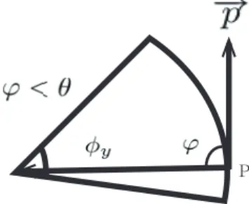
Fig. 2. The sensor’s angle is ϕyand the angle φ between the viewed direction and the facing direction needs to be less than the effective angle θ.
2.3.3 Definition of full view coverage in a period T If during a time period T (T time slots), the network is in the state of full view coverage for at least one time slot, we say the network achieves full view coverage in period T .
2.3.4 Definition of Equivalent Sensing Radius
For heterogeneous camera sensor networks, we define the equivalent sensing radius (ESR) for each static and mobility pattern to analyze the asymptotic full view- coverage. Specifically, the ESR is r = √∑u
y=1cyϕy
2πry2 for static model, and is r = ∑u
y=1cyϕ2πyry for both 1- dimensional and 2-dimensional random walks and the ESR and is r = √∑u
y=1cy(178 −12(32−ϕ2πy)2)r2y for ran- dom rotating mobility model.
In this part,ϕ2πy is viewed as the weight of each sensor’s radius. When ϕ = 2π, it is equivalent to a sensor whose sensing range is a circle, and ESR in this case is reduced to that of omnidirectional sensors [22].
As we mentioned above, we would like to discuss three moving states of sensors. Thus, the motivation of ESR is to unify them as well as present the combination of ry and ϕy of the camera sensor. And our goal is to find a suitable characteristic of sensors to achieve the full view coverage of a given area with a given number of sensors. The critical ESR enables us to find the suitable characteristic of sensors. It is undeniable that there are many alternative indices that can be used. However, the reason that we choose ESR in the present work is that the parameters of both the sensing radius (ry) and viewing angle (ϕy) required in ESR can be easily obtained when we purchase a camera sensor. In this way, we can easily confirm our results in real practice.
Intuitively, the coverage of the network is positively correlated with ESR. The ESR needed when the network exactly achieves asymptotic coverage is called critical ESR, which is defined as follows.
2.3.5 Definition of Critical ESR
Let H denotes the event that the operational region is full view covered. Then
nlim→∞P (H) = 1, if ri≥ cRi(n)for any c > 1;
nlim→∞P (H) < 1, if ri ≤ ˆcRi(n)for any 0 < ˆc < 1,
where Ri(n)is the critical ESR under four different static and mobile patterns, with i =stat, r.r., 2.r.w., 1.r.w., representing the abbreviations of “static model”, “ran- dom rotating mobility model”, “2-dimensional random walk mobility model” and“1-dimensional random walk mobility model”, respectively.
When ESR exceeds the critical one, the operational region will be full covered with probability one when n is sufficiently large, and guarantees the sufficiency of critical ESR. In contrast, when ESR is below the critical value, even though n is large enough, the operational region still cannot be full covered with probability one, which reflects the necessity of critical ESR.
3 O
VERVIEW OF THEG
EOMETRICA
NALYSIS It has been shown in Wang et al. [22] that a dense grid M with√m×√
mis almost always covered when m = n log n. Based on which we can also prove that the θ-view coverage of a facing direction set K formed by k directions of a point can guarantee its full view coverage when k = n log n. Technically, a key factor behind such result lies in the facing direction set of a point. Figure 3 (b) illustrates an example of a facing direction setK of point P . We use k = 8 facing directions to uniformly distribute the angle of circumference into 8 parts. The correlation between full view coverage of P and k directions is presented in Lemma 1.
Tj
j
s
P
0
(a) (b)
a
v b
Fig. 3. (a) A set of four nearest directions including a and bin the direction setK; (b) The possible area Tj to θ-view cover orientation Oj.
Lemma 1: Assume θ, θ0, k are constants and θ0= θ +
2π
k.K is what we shown above. If these k directions can all achieve θ-view coverage, then point P can achieve full view coverage with effective angle θ0.
Proof: Let v be an arbitrary facing direction of point P. Without loss of generality, we assume it is inside the sector formed by virtual orientation a and b in K and is closest to orientation a, as shown in Figure 3 (a).
By assumption, there exists at least one sensor that can cover a, with effective angle θ. Suppose one of them locates at point s (in Figure 3 (a)), and ∠(s, a) < θ. s also represents the viewed direction without confusion.
Besides∠(a, v) < 2πk , then
∠(s, v) = ∠(s, a) + ∠(a, v) < θ +2π
k = θ0. (1) Obviously Eq. (1) still holds when the sensor locates between a and b. Also limk→∞θ0= θ, which means θ0is only slightly larger than θ, when k is large enough. With THEOREM4.1 in [3], the following theorem is derived.
Theorem 1: For point P, if a k facing direction set K satisfies k = n log n, the θ-view coverage of set K can promise the full view coverage of P with effective angle θ when n is large enough.
Thus we can focus on the θ-view coverage of orientation setK for the dense gird M to estimate full view coverage performance of the operational region.
4 C
RITICALS
ENSINGR
ANGE INS
TATICCSN
SWe start with the analysis of full view coverage for static camera sensor networks, and obtain the critical ESR of heterogeneous cameras for coverage with high probability. We also derive the critical equivalent sensing range for almost surely coverage. We first have the following theorem.
Theorem 2: Under the uniform deployment with static model, the critical ESR for static heterogeneous CSNs to achieve asymptotic full view coverage is
Rstat(n) =
√2(log n + log log n)
nθ .
Let Pi,j,Sy denote the probability that orientation Oj of point Piis θ-viewed covered by Sensor S in group Gy. To make Oj of set K θ-viewed covered, at least one sensor should locate in sector Tj, as shown in Figure 3(b). For sector Tj, the angular bisector is orientation j, with an angle 2θ. Then
Pi,j,Sy =P(S falls in Tj)× P(S has proper orientation)
= 2θ
2π× πr2y(n)×ϕy
2π = r2y(n)ϕyθ 2π 4.1 Necessary Condition of Theorem 2
Let Gstat(n, u) denote the network that each point inM achieves full view coverage when the category of sensors is u. And we use Pf−stat(n, u)to represent the probabil- ity that Gstat(n, u) has at least one point that is not full view covered. Then we derive the following proposition.
For simplicity, we say a direction uncovered and not θ- view covered equivalently, and a point uncovered and not full view covered interchangeably. To simplify the proof, we define a variable ω(n) to combine the rstat(n) with the Rstat(n).
Proposition 1: In the static heterogeneous CSN, if rstat(n) =
√2(log n + log log n + ω(n))
nθ ,
m = n log nand k = n log n, then lim inf
n→∞ Pf−stat(n, u)≥ e−2ω−θ πe−3ω, where ω = limn→∞ω(n).
Proof: To simplify the complexity of the proof, we provide the following lemma first.
Lemma 2: Given a variable x = x(n) satisfies 0 <
x(n) < 12, and a variable y = y(n) > 0, then (1− x)y ∼ e−xy if x2y approaches to zero as n→ ∞.
Using the similar method in the proof of LEMMA 1 [16], the proof of Lemma 2 can easily follow. Then we study
the case that r(n) =
√2(log n+log log n+ω(n))
nθ for a fixed ω.
Referring to Bonferroni inequalities, we get Pf−stat(n, r(n))
≥ ∑
Pi∈M
P({some point Pi is not full view covered})
≥ ∑
Pi∈M
P({Pi is the only uncovered point})
≥ ∑
Pi∈M
∑
Oj∈K
P({only Oj of Pi is uncovered})
≥1 ∑
Pi∈M
∑
Oj∈K
P({Oj of Pi is uncovered})
− ∑
Pi∈M Oj∑̸=Oh
Oj,Oh∈K
P({ Oj and Oh of Pi are uncovered}).
(2) The ≥ is where Bonferroni inequalities applied. For the1 first term of the R.H.S. of Eq. (2)
P({Oj of Pi is uncovered})
≥
∏u y=1
P({Oj is uncovered by sensors in Gy})
=
∏u y=1
(
1−r2y(n)ϕyθ 2π
)cyn
,
(3)
where r
2 y(n)ϕyθ
2π represents the probability that orientation Oj of point Piis θ-viewed covered by Sensor S in group Gy, while cynrepresents the number of sensors in group Gy. Then with Lemma 2 and Eq. (3), we obtain that
∑
Pi∈M
∑
Oj∈K
P({Oj of Pi are uncovered)
≥ mk
∏u y=1
(
1−r2y(n)ϕyθ 2π
)cyn
∼ mke−nθ∑uy=1cyϕy2πry2(n)= mke−nθr2stat(n)
= (n log n)2e−2(log n+log log n+ω)= e−2ω.
(4)
For the second term of the R.H.S. of Eq. (2) P({Oj and Oh of Pi are uncovered})
≤ 2θ 2π
∏u y=1
( 1−3
2
r2y(n)ϕyθ 2π
)cyn
+ (
1− 2θ 2π
)∏u
y=1
(
1− 2r2y(n)ϕyθ 2π
)cyn
,
(5)
where the two terms on the right side correspond to the cases where ∠(Oj, Oh) ≤ 2θ and ∠(Oj, Oh) > 2θ, respectively. For the first term, 32r
2 y(n)ϕyθ
2π is the average area sensors may locate to θ-view cover Oj or Oh. Since the overlapping area between Oj and Oh is a random variable uniformly distributed between 0 and θr2(n), the corresponding possible area is also a random variable, uniformly distributed between r
2 y(n)ϕyθ
2π and 2r
2 y(n)ϕyθ
2π , so
that its expectation is 32r
2 y(n)ϕyθ
2π . The second term can be analyzed in a similar manner.
Then according to Lemma 2 and Eqn. (5), we obtain
∑
Pi∈M Oj∑̸=Oh
Oj,Oh∈K
P({Oj and Oh of Pi are uncovered)
≤ mk22θ 2π
∏u y=1
(2π−32r2y(n)ϕyθ 2π
)cyn
+ mk2 (
1−2θ 2π
)∏u
y=1
(2π− 2r2y(n)ϕyθ 2π
)cyn
∼ mk2θ
πe−3nθ2 rstat2 + mk2 (
1−θ π
)
e−2nθr2stat
= θ πe−3ω+
( 1−θ
π )
e−4ω 1 n log n.
Since we consider the asymptotic coverage prob- lem where the total number of cameras n ap- proaches to infinity, for any fixed ω, we can obtain lim infn→∞Pf−stat(n, u)≥ e−2ω−πθe−3ω. Now we con- sider the ω = lim infn→∞ω(n),which indicates that ω(n) < ω + δ for any δ > 0, for all n > Nδ. Since Pf−stat(n, u) is monotonically decreasing in rstat and thus in ω, we have lim infn→∞Pf−stat(n, u)≥ e−2(ω+δ)−
θ
πe−3(ω+δ), for all n > Nδ.
It has been known that Pf−stat(n, u) is bounded away from zero. Combined with the definition of ESR for static model, we know that rstat ≥ Rstat =
√2(log n+log log n) nθ
is necessary to achieve the full view coverage of M.
Moreover, if sensing range rstat is smaller than
√3 2 of critical ESR of static model, the result can be extended as stated in the following Theorem.
Theorem 3: Under the uniform deployment with static model, if the CSN satisfies rstat(n) <
√
3
2Rstat, there still will be an nonegligible probability that the network is uncovered. So we can say that the rstat(n) >
√3
2Rstat is the necessary condition of Theorem 2
Proof: We denote the event that the operational region with n camera sensors has at least one point that is not full view covered as cHn, and use P( cHn) to represent the corresponding probability.
Assuming rstat(n) = c
√3
2Rstat, and referring to Bon- ferroni inequalities, we get
P( cHn)≥ ∑
Pi∈M
∑
Oj∈K
P({Oj of Pi is uncovered})
− ∑
Pi∈M Oj∑̸=Oh Oj,Oh∈K
P({ Ojand Ohof Piare uncovered})
= mk
∏u y=1
(
1−ry2(n)ϕyθ 2π
)cyn
− mk22θ 2π
∏u y=1
( 1−3
2
ry2(n)ϕyθ 2π
)cyn
− mk2 (
1− 2θ 2π
)∏u
y=1
(
1− 2ry2(n)ϕyθ 2π
)cyn
∼ mke−nθ∑uy=1cyϕy2πr2y(n)− mk2θ
πe−3nθ2 ∑uy=1cyϕy2πry2(n)
− mk2 (
1− θ π
)
e−2nθ∑uy=1cyϕy2πry2(n)
= 1
(n log n)3c2−2 − θ π
1
(n log n)92c2−3 − (
1− θ π
) 1
(n log n)6c2−3. If rstat(n)is smaller than
√3
2Rstat, namely, c < 1, then according to the characteristic of P-series, we know that
∑∞ n=1
P( cHn) >
∑∞ n=1
1
(n log n)3c2−2 −
∑∞ n=1
θ π
1 (n log n)92c2−3
−
∑∞ n=1
( 1− θ
π
) 1
(n log n)6c2−3 >∞.
And{ cHn} is a sequence of independence events. Then using Borel–Cantelli Lemma in [26], we know that
P(lim sup
n→∞
Hcn) = 1,
which means the event cHn will infinitely often happen under an asymptotic network. Namely, when rstat(n)≤
√3
2Rstat, for any N , there is always an n which is larger than N , that event cHnwill happen. Shortly, the network is almost surely uncovered when rstat(n)is smaller than
√
3 2Rstat.
4.2 Sufficient Condition of Theorem 2
Now we turn to explore the sufficient condition. First, we obtain the following proposition.
Proposition 2: In CSN, if n sensors are randomly and uniformly deployed in a unit square, and rstat(n) = cRstat where c > 1, then
lim inf
n→∞ P( bH) = 0. (6)
where bH denotes the event that the operational region is not full view covered as defined in Section 2.
The proof is easy to complete so we skip it here due to space limitations. Then from Proposition 2 and the definition of critical ESR for static model, we know that rstat ≥ Rstat =
√2(log n+log log n)
nθ is sufficient to achieve the full view coverage of M. Based on that, we can further obtain the result where sensing range is larger than critical ESR in static network, as is stated in Theorem 4.
Theorem 4: Under the uniform deployment with static model, if the CSN satisfies rstat(n) > cRstat, c > 1, then it is sufficient for the network to achieve full coverage.
4.3 Critical ESR for Full View Coverage of the Oper- ational Range
So far we have already proved that Rstat =
√2(log n+log log n)
nθ is the sufficient condition to achieve full
view coverage for dense gridM. Referring to LEMMA3.1 in [3], as well as Lemma 1 and Theorem 1 in this paper and using similar approach as THEOREM 4.1 in [3], the density of the dense grid m = n log n and the density of the orientation set k = n log n are sufficiently large to evaluate the full view coverage of the whole area.
Moreover, referring to Theorems 3 and 4, we conclude that Ra.s.c.=
√
3
2Rstat is the critical condition to achieve almost surely coverage for static model.
5 T
HEC
RITICALS
ENSINGR
ANGE FORM
O-
BILE
CSN
SNow we proceed to investigate full view coverage prob- lem for CSNs under uniform deployment mobile scenar- ios. Recall that we particularly consider three different mobile patterns, namely, 2-dimensional random walk mobility model, 1-dimensional random walk mobility model and random rotating mobility model.
5.1 Critical ESR Under 2-Dimensional Random Walk We investigate full view coverage in one time slot un- der 2-Dimensional Random Walk Mobility Model, and Figure 4 illustrates the effect of random walk mobility of the sensor on area coverage. We will first analyze full view coverage for dense grid M, and then expand it to the whole area.
Theorem 5: Under the uniform deployment with 2- dimensional random walk mobility model, the critical ESR for mobile heterogeneous CSNs to achieve asymp- totic full view coverage is
R2.r.w(n) =
{ log n+log log n
2nT v sin θ if θ <π2
log n+log log n
2nT v if θ≥π2 .
We will focus on the proof of the case where θ < π2, and the proof is similar when θ≥ π2.
5.1.1 Failure Probability of an Orientation inK
LetFi,jdenote the event that orientation Ojof point Piis not θ-viewed covered during the time slot τ , andP(Fi,j) denote the corresponding probability. We use Pi,j,Sy to represent that Oj of point Pi is θ-viewed covered by Sensor S in group Gy. Then we obtain
Pi,j,Sy =(
(θ + α)r2y(n) + 2vT ry(n) sin θ) ϕy
2π. (7)
T3 time
space
2T3 T
0
vT
time T
direction
Fig. 4. T /3, 2T /3 and T ; the right one illustrates the trace of sensor mobility during the whole interval [0, T ). The shadowed disks constitute the area being covered at the given time instant, and the union of the region inside the dotted line and the shadowed disks represents the area being covered during the time interval.
Fig. 5. Illustration of calculating the mobility area. It is difficult to calculate the mobility area directly, so we rearrange the area into a square and then can easily obtain the result.
In Eq. (7), (θ + α)r2y(n) + 2vT ry(n) sin θrepresents the possible area the sensor may locate in order to θ-view cover Ojduring T slots, if it does not change its direction during the process. (Similarly as we can see from the Fig.
5 that the Eq. (7) can change into (θ+α)ry2(n)+2vT ry(n).) In this formula θr2y(n)represents the possible area where sensors in group Gy, y = 1, 2, .., u might locate if it is stationary,like sector Tj in Figure 3. αr2y(n) represents the additional area due to rotation, which is caused by the sensor’s initial orientation and its chosen direction δ.
Considering its mobility character, the possible area can be 2vT ry(n) sin θmore, like the region inside the dotted line in Figure 4. If the sensor changes its direction during this period, the sensing area will overlap, making it no larger than 2vT ry(n) sin θ. For formula ϕ2πy, it represents the probability that the sensor in group Gy has proper orientation to sense the point. With all those factors determined, P(Fi,j)can then be calculated.
5.1.2 Necessary ESR for Full View Coverage
Here, we use cHτ to denote the event that the dense grid M is not fully full view covered in the time slot τ, and present the following proposition regarding the necessary condition. We will slightly abuse the notation and use the ω which represent the same meaning as that in Proposition 1
Proposition 3: In the mobile heterogeneous CSN with 2-dimensional random walk mobility model, if r2.r.w.=
log n+log log n+ω(n)
2nT v sin θ and the density of the dense grid M is m = n log n, the density of the orientation set K is k = n log n, then
lim inf
n→∞ Pτ( cHτ)≥ e−2ω−θ πe−3ω, where ω = limn→∞ω(n).
Proof: Similar to the proof of Proposition 1, we first study the case where r2.r.w. = log n+log log n+ω
2nT v sin θ , for a fix ω.
Pτ( cHτ)≥ ∑
Pi∈M
∑
Oj∈K
Pτ({Oj of Pi is uncovered})
− ∑
Pi∈M Oj∑̸=Oh
Oj,Oh∈K
Pτ({Oj and Oh of Pi are uncovered).
(8)
And we calculate that
Pτ({Oj of Pi is uncovered})
=
∏u y=1
( 1−(
(θ + α)r2y(n) + 2vT ry(n) sin θ) ϕy 2π
)cyn
=
∏u y=1
(
1− (1 + λy)ϕyvT ry(n) sin θ π
)cyn
,
where λy = (θ+α)r2vT sin θy(n) = Θ(ry(n)) = o(1), since the asymptotic coverage problem is considered.
Then we can bound the first term of R.H.S of Eq. (8),
∑
Pi∈M
∑
Oj∈K
Pτ({Oj of Pi is uncovered}) (9)
≥mke−4vT sin θn
∑u y=1
cy
ϕy
2πry
=mke−4vT sin θnr2.r.w.
=e−2ω.
Similarly, we bound the second term
∑
Pi∈M Oj∑̸=Oh
Oj,Oh∈K
Pτ({Oj and Oh of Pi are uncovered)∼ θ πe−3ω.
Then we have lim infn→∞Pτ( cHτ)≥ e−2ω−πθe−3ω. Since ω is a function of n, the conclusion holds.
According to Proposition 3, we know that R2.r.w. ≥
log n+log log n+ω(n)
2nT v sin θ is necessary to achieve the full view coverage of M. Moreover, if sensing range is smaller than
√3
2 of critical ESR of the 2-dimensional random walk mobility model, we can extend our result to the following theorem. We omit the proof here since it shares a similar technique adopted in the proof of Theorem 3.
Theorem 6: Under the uniform deployment with the 2- dimensional random walk mobility model, if the CSN satisfies r2.r.w.(n) <
√3
2R2.r.w., there still will be an nonegligible probability that the network is uncovered.
So we can say that the r2.r.w. >
√3
2R2.r.w. is the necessary condition for the network to achieve full view coverage.
5.1.3 Sufficient ESR for Full View Coverage
Before we proceed, we first present the following propo- sition.
Proposition 4: In CSN, if n sensors are randomly and uniformly deployed in a unit square, and r2.r.w.(n) = cR2.r.w.(n)where c > 1, then
lim inf
n→∞ Pτ( cHτ) = 0. (10) The proof can be completed using a similar approach as in Proposition 2 following that fact that Eq. (10) can be