Classification of multispectral images through a rough-fuzzy neural network

(1)

Classification of multispectral images through

a rough-fuzzy neural network

Chi-Wu Mao

National Cheng Kung University Department of Electrical Engineering No. 1, Ta-Hseuh Rd

Tainan, Taiwan Shao-Han Liu

Jzau-Sheng Lin,MEMBER SPIE

National Chin-Yi Institute of Technology Department of Electronic Engineering No. 35, Lane 215, Sec. 1,

Chung-Shan Rd Taiping, Taichung, Taiwan E-mail: jslin@chinyi.ncit.edu.tw

Abstract. A new fuzzy Hopfield-model net based on rough-set reason-ing is proposed for the classification of multispectral images. The main purpose is to embed a rough-set learning scheme into the fuzzy Hopfield network to construct a classification system called a rough-fuzzy Hopfield net (RFHN). The classification system is a paradigm for the implementation of fuzzy logic and rough systems in neural network ar-chitecture. Instead of all the information in the image being fed into the neural network, the upper- and lower-bound gray levels, captured from a training vector in a multispectal image, are fed into a rough-fuzzy neuron in the RFHN. Therefore, only 2/N pixels are selected as the training samples if anN-dimensional multispectral image was used. In the simu-lation results, the proposed network not only reduces the consuming time but also reserves the classification performance. ©2004 Society of Photo-Optical Instrumentation Engineers. [DOI: 10.1117/1.1629685]

Subject terms: rough set; fuzzy Hopfield neural network; multispectral images. Paper 030172 received Apr. 14, 2003; revised manuscript received Jul. 10, 2003; accepted for publication Jul. 10, 2003.

1 Introduction

Multispectral classification has been described as generat-ing better discrimination than sgenerat-ingle spectral classification.1 In the remotely sensed images, the multispectral images are extracted from multiple-band sensors operated from either a spaceborne or an airborne platform such as the Landsat seven-band thematic mapper 共TM兲, the four-band multi-spectral scanner 共MSS兲, and the three-band Satellite Pour 1’Observation de la Terra 共SPOT兲. In other words, mag-netic resonance imaging共MRI兲 systems can produce multi-band images, each of which emphasizes a different funda-mental parameter of internal anatomical structures in the same body section with multiple contrasts, based on local variations of spin-lattice relaxation time (T1), spin-spin re-laxation time (T2), and proton density共PD兲. The classifi-cation of multispectral images has been successfully em-ployed in the past.1– 8 The analysis of such multidimensional images can be accomplished by using su-pervised or unsusu-pervised classification methods. In super-vised classification strategies, the region of interest共ROI兲 is defined by the associated human interaction and the ap-proach trains on the ROI and flags each pixel in the scenes associated with a given signature. However, a supervised approach is very time-consuming for large volumes and heavy biases may be introduced by an unskilled technician. The unsupervised classification methods classify the multi-dimensional data sets without the aid of training sets, but a postprocessing step is required to correct misclassified pix-els.

Generally speaking, unsupervised classification ap-proaches such as hard c-means 共HCM兲共Ref. 9兲 and ISODATA共Ref. 10兲 are traditional clustering methods in which each sample belongs only to one cluster. Fuzzy clus-tering methods11–13 共FCM兲 Penalized FCMs 共PFCMs兲

共Refs. 14 and 15兲, and compensated FCMs 共CFCMs兲共Ref. 16兲 are methods in which every sample belongs to all clus-ters with different degrees of membership.

Rough set theory, proposed by Pawlak,17,18 provides a systematic framework for the study of the problems arising from imprecise and insufficient knowledge. Instead of fuzziness dealing with vagueness between the overlapping sets19,20and fine concepts, the rough sets deal with coarse nonoverlapping concepts. In fuzzy sets, each training sample can have only one membership value to a particular class. However, rough sets declare that each training sample may have different membership values to the same class. Therefore, rough sets are of interest to deal with a classification system, in which knowledge about the system is unrefined.

Applications of neural-network-based approaches to pat-tern classification have been extensively studied in the last couple of decades. In the application of multispectral image classification, neural networks exploit the massive parallel-ism of neurons. Ozkan et al.6 proposed a neural-network-based segmentation of multimodal medical image. To up-date the performance, fuzzy reasoning algorithms have been added into neural network to construct fuzzy-neural systems.7,8,16Lin et al.7,8presented a penalized fuzzy com-petitive learning network and a fuzzy Hopfield neural net-work 共FHNN兲 to three-band and five-channel magnetic resonance image classification, respectively. Lin16also em-bedded the compensated fuzzy c-means into a Hopfield net and applied it to clustering. These networks proved that better segmentation results are offered than those from a single modality. In this paper, we extended the author’s method in Refs. 7 and 8 to multiband image segmentation. The rough-set learning is added into Fuzzy Hopfield net-work to construct the rough-fuzzy Hopfield netnet-work 共RFHN兲 for classification of multispectral images. Instead

(2)

of only one state for a neuron, the membership state is used in the FHNN, the proposed RFHN occupies two states termed as upper- and lower-bound membership states. This approach has two advantages, namely, it is more robust to computing efficient and it is an unsupervised algorithm based on a neural network.

The rest of this paper is organized as follows. Section 2 reviews the cluster techniques with rough-fuzzy concept. Section 3 presents the RFHN. Section 4 shows several ex-perimental results. Finally, Sec. 5 gives the discussion and conclusions.

2 Rough Set Theory

Let R be a binary equivalence relation defined on a univer-sal set Z is a subset of the Cartesian product, R債Z⫻Z. An equivalence relation is a binary relation R that satisfies

R is reflexive: z₁苸Z→共z₁,z₁兲苸R,

R is symmetric: 关z₁,z₂苸Z∧共z₁,z₂兲苸R兴→共z₂,z₁兲苸R,

R is transitive: 关z₁,z₂,z₃苸Z∧共z₁,z₂兲苸R∧共z₂,z₃兲 苸R兴→共z1,z3兲苸R.

Let z苸Z, let 关z兴 be the equivalence class containing z, and let Z/R denote the family of all equivalence classes induced on Z by R. There exists an equivalence class in Z/R, des-ignated by关z兴R, that contains a training sample z苸Z. For any output class A債Z, the lower approximation Rគ(A) and upper approximation R¯ (A) are defined as subsets of A and they approach A as closely as possibly from inside and outside in the set respectively. Therefore, Rគ (A) can be de-fined as the union of all equivalence classes in Z/R that are contained in A such that

Rគ 共A兲⫽艛兵关z兴R兩关z兴R債A, z苸Z其, 共1兲

whereas R¯ (A) can be also defined as the union of all equivalence classes in Z/R that overlap with A like the following equation

R

¯_{共A兲⫽艛}_兵_关z兴

R兩关z兴R艚A⫽␾, z苸Z其. 共2兲

A rough set can be represented by Rគ (A) and R¯(A) with the given set A as

R共A兲⫽

具

R¯共A兲,Rគ共A兲

典

. 共3兲

And the rough boundary of A by the equivalence classes

Z/R is distinct as

RB共A兲⫽R¯共A兲⫺Rគ共A兲. 共4兲

The rough or rough-fuzzy neural networks have been proposed in the last decade. In 1998, Lingras21,22proposed

three models of rough neurons. The value in a rough pat-tern is a pair of upper and lower bounds. A rough neuron s can be viewed as a pair of neurons called upper-bound neuron (s¯) and lower-bound neuron (sគ) to receive a pair of

patterns. A full-connected model that displays a rough neu-ron r connects to a proper rough neuneu-ron s with four con-nections. If the rough neuron r excites the activity of s, the connections from r¯ to s¯ and from rគ to sគ are created

respec-tively. On the other hand, if r inhibits the activity of s, the connections from r¯ to sគ and from rគ to s¯ are created,

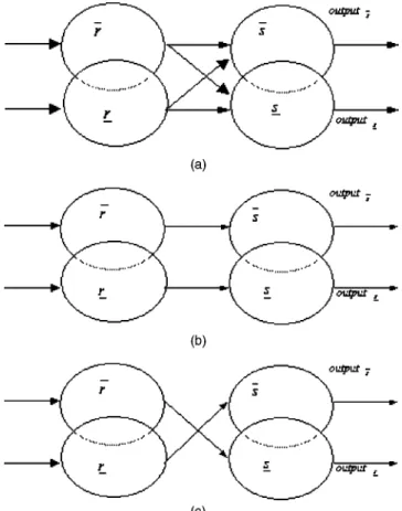
respec-tively. These three model neurons are shown in Fig. 1. In this paper, the excited-model rough neuron, shown Fig.

Fig. 1 Interconnection in the architecture of rough neurons: (a) fully

connected, (b) exciting model, and (c) inhibiting model.

Fig. 2 Architecture of a neuron (x,i) in the 2-D RFHN. Mao, Liu, and Lin: Classification of multispectral images . . .

(3)

1共b兲, is applied into the neurons in the RFHN due to it getting a better performance. Therefore, the inputs in the excited-model rough neuron are

input¯s⫽

兺

r⫽1 m w¯,r¯s output¯r, 共5兲 and inputsគ⫽

兺

r⫽1 m wsគ,rគoutputrគ. 共6兲

The outputs of a rough neuron s are expressed using an activation function as

output¯_s⫽max关t共input¯s兲,t共inputsគ兲兴, 共7兲 and

outputsគ⫽min关t共input¯s兲,t共inputsគ兲兴, 共8兲 where the activation function can be defined as

t共x兲⫽ 1

1⫹e⫺␬x 共9兲

and␬is a constant with a range from 0 to 1.

(4)

3 Rough-Fuzzy Hopfield Neural Network

The Hopfield-model neural networks23,24have been studied extensively. The features of this network are simple and have clear potential for parallel implementation. To im-prove the performance in the application of optimal prob-lems, modified Hopfield networks7,8,16,25,26 have been pro-posed. Lin et al.7,8 Lin,16 and Lin and Liu25 proposed different fuzzy Hopfield networks to the applications of clustering problem and medical image segmentation. These modified Hopfield networks are based on fuzzy reasoning. In the Refs. 7, 8, 16, and 26, each neuron occupies only one state, which is updated with a membership grade. For the purpose of updating the computing performance, the rough-set strategy is embedded into a fuzzy Hopfield network to

construct the RFHN in this paper. Instead of updating and memorizing the centroids for iteratively training samples in the FHNN, the neuron states and synaptic weights are up-dated with rough-fuzzy strategy in the modified Hofield net. Finally, the centroids are calculated using the training samples, and upper- and lower-bound states when the en-ergy is converged. In the RFHN, as shown in Fig. 2, each neuron occupies two inputs called lower- and upper-inputs and two output states called upper- and lower-bound mem-bership states based on all c cluster’s centers. Thus these two inputs for neuron (x,i) and Lyapunov energy function in the 2-D RFHN can be modified from conventional Hopfield net as

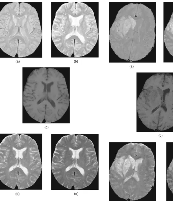
Fig. 4 Multi-spectral MRI head images with normal physiology: (a) TR1/TE1⫽2500 ms/25 ms, (b) TR2/TE2⫽2500 ms/50 ms, (c)

TR3/TE3⫽500 ms/11.9 ms, (d) TR4/TE4⫽2500 ms/75 ms, and (e)

TR5/TE5⫽2500 ms/100 ms.

Fig. 5 Multispectral MR head images with cerebral infarction: (a) TR1/TE1⫽2500 ms/25 ms, (b) TR2/TE2⫽2500 ms/50 ms, (c)

i⫽1 c

共Iគx,i␮គx,i m_⫹I¯

x,i␮¯x,i m

兲, 共12兲

where 兺_yn_⫽1Wគx,i;y ,i and 兺y⫽1 n

W¯x,i;y ,i are the total lower-and upper-bound interconnected weights received from the

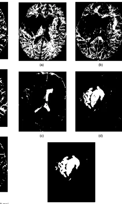
Fig. 6 Classified images in channel 5 with TR5/TE5⫽2500 ms/

100 ms: pictures (a) GM, (c) WM, and (e) CSF are classified by RFHN and (b) GM, (d) WM, and (f) CSF are classified using FHNN,

respectively. Fig. 7 Classified images using the proposed RFHN in channel 2_{with TR}

2/TE2⫽2500 ms/50 ms: (a) GM, (b) WM, (c) CSF, (d) CI,

(6)

2 ⫹C₂

, 共13兲 where ERFHNis the objective function that accounts for the energies of all training samples in the same class.

The first two terms in Eq.共13兲 define the Euclidean dis-tance between the training samples in a cluster and that cluster’s centers over c clusters with the lower- and upper-bound membership grades for all neurons. The third and fourth terms guarantee that n training samples in Z are distributed among these c clusters. More specifically, these two terms共the constrained term兲, impose constraints on the objective function, and the first and second terms minimize the intraclass Euclidean distance from training samples to the cluster centers in lower- and upper-bound data sets, respectively.

All the neurons in the same row compete with one an-other to determine the training sample represented by that row belongs to all clusters with lower- and upper-bound membership grades, respectively. In other words, the sum-mation of the membership states for different bounds in the same row equals 1. That is the total sum of membership states in all n rows equal n for individual bound. This as-sures that all n samples will be classified into c classes. The objective function in the RFHN can be further simplified as

2 . 共14兲

By using Eq.共14兲, the minimization of ERFHNis greatly simplified, since Eq.共14兲 contains only two term, the need to find the weighting factors A, B, C, and D are removed. Comparing Eq. 共14兲 with the modified Lyapunov function Eq.共12兲, the synaptic interconnection weights and the bias inputs for the proposed RFHN can be obtained as

Fig. 8 Classified images CI with median filter using FHNN.

Table 1 The average computation time (five experiments) required to classify the simulated multispectral images for FHNN and the proposed RFHN (in seconds).

Algorithm

Normal Mutispectral MRI Images (Fig. 3)

Multispectral MRI head Images with Cerebral Infarction (Fig. 6)

FHNN 36.8 27.0

RFHN 24.0 19.8

Table 2 The simulating cluster centers of different objects for vari-ant channels in test phvari-antons, which are the average values esti-mated from 10 multispectral MRI head images with normal physiol-ogy using the same parameters in Fig. 4.

Channels Objects CH1 CH2 CH3 CH4 CH5 BKG 0 0 0 0 0 GM 192 183 91 152 108 WM 166 159 103 108 75 CSF 203 248 68 220 199

(7)

Wគx,i;y ,i⫽ ␮គy ,i m 兺h⫽1 n _共_␮_គ h,i m _兲, 共15兲 W¯x,i;y ,i⫽ 共␮¯_{y ,i}m兲兺h⫽1 n 共␮¯_h,im 兲, 共16兲 I គx,i⫽0, 共17兲 and I ¯ x,i⫽0 共18兲

By introducing Eqs.共15兲, 共16兲, 共17兲, and 共18兲 into Eqs. 共10兲 and 共11兲, the lower- and upper-bound total inputs of neuron (x,i) can be expressed as

2 . 共20兲

Consequently, the lower- and upper-bound output states at neuron (x,i) in the RFHN are given by

␮គx,i⫽min共␶គx,i,¯␶x,i兲, 共21兲

and

␮

¯_x,i⫽max共␶គ_x,i,¯␶_x,i兲, 共22兲

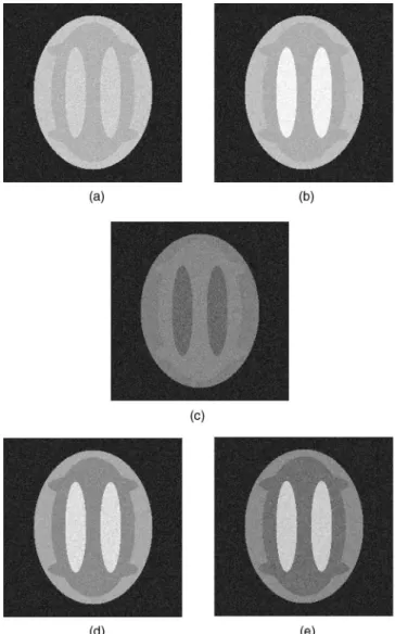
Fig. 9 Test phantoms for simulating different objects (BKG, GM, WM, and CSF) in meltispectral image.

Fig. 10 Test phantoms for simulating different objects (BKG, GM, WM, and CSF) in meltispectral image with adding Gaussian noise ␦⫽⫾30.

(8)

where the active function at a rough-fuzzy neuron (x,i) in the RFHN are defined as

␶គx,i⫽

冋

兺

j⫽1 c

冉

Netx,i Netx, j

冊

1/m⫺1

册

⫺1 for all i, 共23兲 and ␶ ¯x,i⫽

冋

兺

j⫽1 c

冉

Netx,i Netx, j

冊

1/m⫺1

册

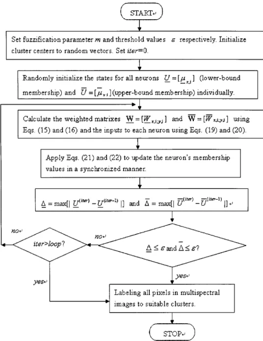
⫺1 for all i. 共24兲

The training samples of the lower- and upper-bound in-puts for a rough-fuzzy neuron in the 2-D RFHN were ex-tracted from a five-component vector in a 5-D multispectal image. Therefore directly mapping the lower- and upper-bound training samples to the 2-D rough-fuzzy neuron ar-ray, the RFHN is trained to update all neuron states in order to classify the input vectors into feasible clusters when the defined energy function converges to near global minimum. The detailed process of the RFHN is shown in Fig. 3, in which parameters iter and maxi are number of iterations and maximum value of iteration respectively.

4 Experimental Results

To show the classification and computation performance, all simulations are executed with the interpreter language of MATLAB in a Pentium III personal computer. Due to the noise in acquisition and of the partial volume effects from the low resolution of the sensors, the uncertainty is widely present in medical images. The unsupervised approaches based on fuzzy clustering techniques are particularly suit-able for handling a decision-making process in classifica-tion of multimodal medical images. These real medical

im-ages in Figs. 4 and 5 are acquired with T2-weighted sequences for channel images CH⫽1, 2, 4, and 5 and

T1-weighted signal for channel image CH⫽3, respectively. The acquisition parameters with different repetition time 共TR兲 and echo time 共TE兲 are TR1/TE1⫽2500 ms/25 ms, TR₂/TE₂⫽2500 ms/50 ms, TR₃/TE₃⫽500 ms/11.9 ms, TR₄/TE₄⫽2500 ms/75 ms, and TR₅/TE₅⫽2500 ms/ 100 ms for Fig. 4; and TR₁/TE₁⫽2500 ms/25 ms, TR₂/ TE₂⫽2500 ms/50 ms, TR₃/TE₃⫽500 ms/20 ms, TR₄/ TE4⫽2500 ms/75 ms, and TR5/TE5⫽2500 ms/100 ms for Fig. 5 individually. A training vector consisting of lower-and upper-bound samples that are extracted from five com-ponents in a multispectral image and directly fed into a row of the RFHN.

The first example is multispectral image classification in MR head images of a normal physiology shown in Fig. 4. In Fig. 6, different regions were classified by the RFHN and FHNN from Fig. 4 such as background 共BKG兲, gray matter共GM兲, white matter 共WM兲, and cerebral spinal fluid 共CSF兲, respectively. From Fig. 6, we almost cannot distin-guish the classified tissues by the RFHN from the FHNN.

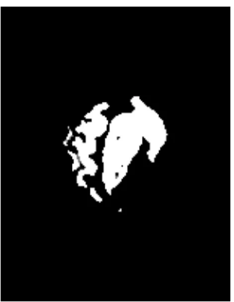
The second example is a multispectral image classifica-tion in MRI head image of a patient diagnosed with cere-bral infarction shown in Fig. 5. Figure 7 shows the five regions BKG, GM, WM, CSF, and cerebral infarction共CI兲 classified by the RFHN, respectively. After a postprocess-ing with median filterpostprocess-ing, the detail of an abnormal region with cerebral infarction is displayed in Fig. 7共e兲. Figure 8 also shows the abnormal region with CI classified by the FHNN and a postprocessing with the median filter. The classified CI region by using the proposed RFHN is a little different from that segmented by the FHNN. These results are acceptable for the future processing.

Table 3 The segmentation performances in error detecting pixels for FHNN and RFHN methods using the simulated image with␦⫽⫾20.

Simulation Object Actual Pixels FHNN RFHN

Background (BKG) 36,189 36,189 36,189

GM 9538 9538 9538

WM 13,711 13,710 13,710

CSF 6098 6098 6098

Misclassified pixels 0 1 1

Total error ratio 1/65,536⫽0.0% 1/65,536⫽0.0%

Background (BKG) 36,189 36,189 36,189

GM 9538 8689 8654

WM 13,711 11,976 12,183

CSF 6098 6087 6096

Misclassified pixels 0 2595 2529

Total error ratio 2595/65,536⫽3.96% 2529/65,536⫽3.86% Mao, Liu, and Lin: Classification of multispectral images . . .

(9)

To emphasize the classification ability of the proposed RFHN, several test phantoms were constructed for simula-tion. Every test phantom was made up of six overlapping ellipses in the last experiment. Each ellipse represents one structural area of tissue. From periphery to the center, they were the background 共BKG, 36,189 pixels兲, gray matter 共GM, 9538 pixels兲, white matter 共WM, 13,711 pixels兲, and cerebrospinal fluid 共CSF, 6098 pixels兲, respectively. The cluster centers for different channels in test phantoms, shown in Table 2, are the average values estimated from 10 sets of multispectral MRI head images with normal physi-ology using the same parameters as in Fig. 4. The computer-generated images to simulate variant channels are shown in Fig. 9. In addition, a Gaussian distribution noise with gray levels ranging from⫺␦ to⫹␦ was added to test phantoms. The test phantoms with Gaussian distribution noise␦⫽⫾30 for different channels are shown in Fig. 10. The classified results of test phantoms with variant noises

␦⫽⫾20, ⫾30, and ⫾80 are displayed in Tables 3, 4, and 5, respectively. In the proposed RFHN, the test multispec-tral phantoms were divided into nonoverlapped blocks with a size of 2⫻2 pixels to determine the maximum and mini-mum values as the upper- and lower-bound training vec-tors. Therefore, only one half of the pixels of an image are used in the last experiment. The simulated-structural areas of tissues can be completely and correctly classified when the Gaussian noise is兩␦兩⭐10 for both RFHN and FHNN. As shown in Tables 3, 4, and 5, the proposed RFHN can obtain more promising classification performance than the FHNN. For example, 2595 pixels were misclassified with a

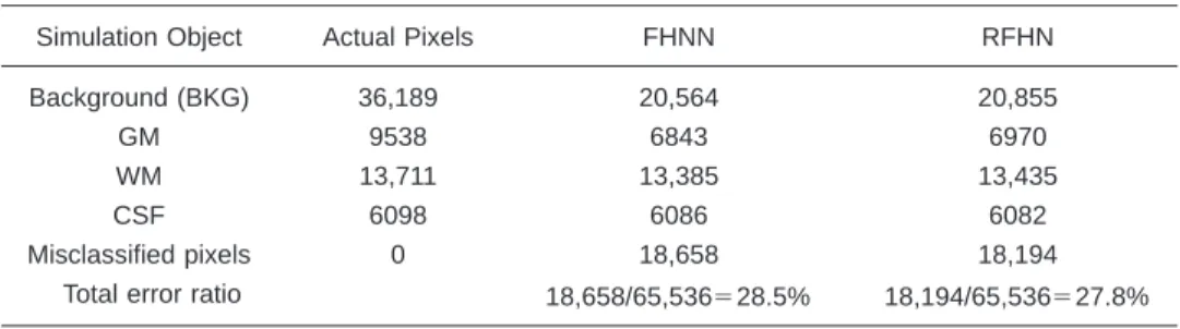
3.96% error rate using FHNN while 2529 pixels were mis-classified with 3.86% error rate using the RFHN by ␦ ⫽⫾30. The total misclassified pixels for the test phantoms with␦⫽⫾80 were 18,658 and 18,194 using FHNN and the proposed RFHN, respectively. The classified regions are shown in Fig. 11 with Gaussian distribution noise ␦⫽ ⫾30 using FHNN and RFHN. The better classification per-formance can be clearly displayed by the RFHN than those yielded by the FHNN.

5 Conclusions

A modified Hopfield net model called the RFHN with an embedded rough-fuzzy reasoning strategy was proposed for the classification of multispectral images. Every neuron in the proposed RFHN owns two sampling inputs, two bias inputs, and two output states termed lower- and upper-bound membership states. In the application of 5-D multi-spectral image classification, only 2/5 information extracted from a target image as training samples. Therefore, the computation performance can be updated compared with the FHNN. To update the classification performance, the test image can also be divided into several nonoverlapped blocks. We can determine maximum and minimum norms in a blocked-vector as the upper- and lower-bound training vector. In the blocked manner, not only are the training vectors reduced, but the classification performance is pre-served.

Acknowledgment

This work was supported by the National Science Council, Taiwan, under the Grant No. NSC90-2213-E-167-003. References

1. M. Vannier, T. Pilgram, C. Speidel, L. Neumann, D. Rickman, and L. Schertz, ‘‘Validation of Magnetic resonance imaging 共MRI兲 multi-spectral tissue classification,’’ Comp. Med. Imaging Graph. 15, 217– 228共1991兲.

2. C.-I. Chang and C. Brumbley, ‘‘A Kalman filtering approach to mul-tispectral image classification and detection of changes in signature abundance,’’ IEEE Trans. Aerosp. Electron. Syst. 37, 257–268共1999兲. 3. A. Ifarraguerri and C.-I. Chang, ‘‘Multispectral and hyperspectral im-age analysis with convex cones,’’ IEEE Trans. Geosci. Remote Sens.

37, 756 –770共1999兲.

4. T. Taxt and A. Lundervold, ‘‘Multispectral analysis of the brain using magnetic resonance imaging,’’ IEEE Trans. Med. Imaging 13, 470– 481共1994兲.

5. M. W. Vannier, R. L. Butterfield, D. Jordan, W. A. Murphy, R. G. Levitt, and M. Gado, ‘‘Multispectral analysis of magnetic resonance images,’’ Radiology 154, 221–224共1985兲.

6. M. Ozkan, B. M. Dawant, and R. J. Maciunas, ‘‘Neural-network-based segmentation of muliti-modal medical images: a comparative and prospective study,’’ IEEE Trans. Med. Imaging 12, 534 –544 共1993兲.

Fig. 11 Classified regions using different approaches with adding Gaussian noise␦⫽⫾30: (a) FHNN and (b) RFHN.

Background (BKG) 36,189 20,564 20,855

GM 9538 6843 6970

WM 13,711 13,385 13,435

CSF 6098 6086 6082

Misclassified pixels 0 18,658 18,194

(10)

7. J.-S. Lin, K.-S. Cheng, and C.-W. Mao, ‘‘Segmentation of multispec-tral magnetic resonance images using penalized fuzzy competitive learning network,’’ Comput. Biomed. Res. 29, 314 –326共1996兲. 8. J.-S. Lin, K.-S. Cheng, and C.-W. Mao, ‘‘Multispectral magnetic

reso-nance images segmentation using fuzzy Hopfield neural network,’’

Int. J. Bio-Med. Comput. 42, 205–214共1996兲.

9. G. H. Ball and D. J. Hall, ‘‘A clustering technique for summarizing multivariate data,’’ Behav. Sci. 12, 153–155共1967兲.

10. J. C. Dunn, ‘‘A fuzzy relative of the ISODATA process and its use in detecting compact well-separated clusters,’’ J. Cybernet. 1共3兲, 32–57 共1974兲.

11. H. J. Zimmermann, Fuzzy Set Theory and Its Application, Cluwer, Boston共1991兲.

12. M. A. Ismail and S. Z. Selim, ‘‘Fuzzy c-mean: optimality of solutions and effective termination of the algorithm,’’ Pattern Recogn. 19, 481– 485共1986兲.

13. J. C. Bezdek, ‘‘Fuzzy mathematics in pattern classification,’’ PhD Dis-sertation, Applied Mathematics, Cornell University, Ithaca, NY 共1973兲.

14. M.-S. Yang, ‘‘On a class of fuzzy classification maximum likelihood procedures,’’ Fuzzy Sets Syst. 57, 365–375共1993兲.

15. M.-S. Yang and C.-F. Su, ‘‘On parameter estimation for normal mix-tures based on fuzzy clustering algorithms,’’ Fuzzy Sets Syst. 68, 13–28共1994兲.

16. J.-S. Lin, ‘‘Fuzzy clustering using a compensated fuzzy Hopfield net-work,’’ Neural Process. Lett. 10, 35– 48共1999兲.

17. Z. Pawlak, ‘‘Rough sets,’’ Int. J. Inf. Comput. Sci. 11, 145–172 共1982兲.

18. Z. Pawlak, ‘‘Rough classification,’’ Int. J. Man-Mach. Stud. 20, 469– 483共1984兲.

19. D. Dubois and H. Prade, ‘‘Rough fuzzy sets and fuzzy rough sets,’’

Int. J. Gen. Syst. 17, 191–209共1990兲.

20. G. S. Klir, B. Yuan, Fuzzy Sets and Fuzzy Logic—Theory and

Appli-cations, Prentice-Hall, Englewood Cliffs, NJ共1995兲.

21. P. Lingras, ‘‘Comparison of neofuzzy and rough neural networks,’’

Inf. Sci. (N.Y.) 110, 207–215共1998兲.

22. P. Lingras, ‘‘Fuzzy-rough and rough-fuzzy serial combinations in neu-rocomputing,’’ Neurocomputing 36, 29– 44共2001兲.

23. J. J. Hopfield, ‘‘Neural networks and physical systems with emergent collective computational abilities,’’ Proc. Natl. Acad. Sci. U.S.A. 79, 2554 –2558共1982兲.

24. J. J. Hopfield and D. W. Tank, ‘‘Neural computation of decisions in optimization problems,’’ Biol. Cybern. 52, 41–152共1985兲.

25. J.-S. Lin and S.-H. Liu, ‘‘A competitive continuous Hopfield neural network for vector quantization in image compression,’’ Eng. Applic.

Artif. Intell. 12, 111–118共1999兲.

26. J.-S. Lin, K.-S. Cheng, and C.-W. Mao, ‘‘A fuzzy Hopfield neural network for medical image segmentation,’’ IEEE Trans. Nucl. Sci. 43, 2389–2398共1996兲.

27. A. Kanstein, M. Thomas, and K. Goser, ‘‘Possibilistic reasoning neu-ral network,’’ in Proc. IEEE Int. Conf. on Neuneu-ral Networks 4, 2541– 2545共1997兲.

Chi-Wu Mao is an associate professor with the Department of Electrical Engineering, National Cheng Kung University, Tainan, Taiwan. He received his BS degree in elec-trical engineering from National Cheng Kung University in 1963 and his MS de-grees in electrical engineering from Purdue University in 1970. He was a research fellow with Hannover University, Germany, in 1981. His research interests involve im-age processing, pattern recognition, and medical image analysis.

Shao-Han Liu is a lecturer with the De-partment of Electronic Engineering, Na-tional Chin-Yi Institute of Technology, Tai-chung, Taiwan. He received his BS degree in electronic engineering from Taiwan Uni-versity of Science and Technology in 1983 and his MS degree in management sci-ence from Northrop University in 1989. His research interests involve neural networks and image compression.

Jzau-Sheng Lin is a professor with the Department of Electronic Engineering, Na-tional Chin-Yi Institute of Technology, Tai-chung, Taiwan. He received his BS degree in electronic engineering from Taiwan Uni-versity of Science and Technology in 1980 and his MS and PhD degrees in electrical engineering from National Cheng Kung University in 1989 and 1996, respectively. He is a member of SPIE and his research interests involve neural network, image compression, pattern recognition, and medical image analysis. Mao, Liu, and Lin: Classification of multispectral images . . .