The Effect of Preprocessing on Neural Network for Short- Term Electricity Load Forecasting

1. Introduction

The issue of power supply has received more and more attention with increasing power demand for economy growth. Renewable energy has been the focus in pursuing sustainable future. However, renewable capacity additions cause several challenges: increasing power grid complexity for energy distribution, volatile load swings, frequency and voltage for management that require fast reacting grid control and adaptive assets. An accurate short-term load forecasting is therefore important to balance the demand and supply sides.

Load forecasting is usually concerned with the prediction of hourly, daily, weekly, and annual values of the system demand and peak demand.

Such forecasts are sometimes categorized as short- term, medium-term, and long-term forecasts, depending on the time horizon. In terms of forecasting outputs, load forecasts can also be categorized as point forecasts (i.e., forecasts of the mean or median of the future demand distribution), and density forecasts (providing estimates of the full probability distributions of the possible future values of the demand). Long-term forecasts usually require more than merely an extrapolation of the seasonality or trend evident in the historical data. A forecasting tool can not only derive a forecast from outside explanatory variables, such as economic or demographic information, but also help account for changes in the historical data and be a predictor in the forecast period. For instance, in electric load

Volume 6, No. 2, June 2019, pp. 103-117

The Effect of Preprocessing on Neural Network for Short- Term Electricity Load Forecasting

Chuen-Jyh Chen

Chieh-Hsin Hsu

Kai-Wei Yu

Shih-Ming Yang

ABSTRACT

A short-term load forecasting neural network model based on rough sets is established to predict future power demand one day to one week ahead. The model is validated by a set of data including both weather factors from Central Weather Bureau and history load from Taiwan Power Company. Rough set is applied to modify the model by eliminating redundant attributes. The impact of preprocessing increases the reliability of the neural network model, which successfully avoids the complexity of the system; hence it performs better than the traditional neural network model. The model for forecasting is simulated in MATLAB and the results can increase the reliability of power system to further help energy economic and strategy planning.

Keywords:

Received Date: June11, 2018 Revised Date: November 12, 2018 Accepted Date: December 3, 2018

1 Associate Professor, Department of Aviation and Maritime Transportation Management, Chang Jung Christian University, Taiwan, R.O.C.

2 Graduate, International Bachelor Degree Program on Energy Engineering, National Cheng Kung University, Taiwan, R.O.C.

3 Professor, Department of Aeronautics and Astronautics, National Cheng Kung University, Taiwan, R.O.C.

* Corresponding Author, Phone: +886-6-2785123#2260, E-mail: [email protected]

forecasting, short-term forecasts are influenced by weather conditions (driving air conditioning loads and heating use), whereas long-term forecasts are dominated by economic development and political decisions (building offshore wind parks yields different load distributions than those yielded by power plants). The forecasting model presented in this paper is suitable for short-term forecasts;

therefore, there are few available socio–economic variables, which are different from the variables used in most methods that are used for long-term forecasts. There is no common basis to compare the prediction performance of models. Even for short-term forecasts, it is difficult to predict electrical loads because of many influencing social, weather, and seasonal factors. Social factors include human activities such as attending work or school, and they may affect the electricity supply.

Weather factors include temperature and humidity, and these influence residential load. Seasonal factors include the trend of the four seasons and yearly power demand growth. The production of too much energy is wasteful and increases operational cost. Conversely, the insufficiency of electricity directly and severely affects the national economy. Thus, a robust short-term load forecasting model is crucial to precisely dispatch power during transmission and distribution.

Various forecasting methods have been developed for forecasting. Similar day forecast (Chen et al., 2010) uses daily load patterns, categorized by day type and month, and load increment patterns to compute a future day’s load forecast. Kalman filter with adaptive quality (Takeda et al., 2016) is used for estimating electricity load. In the early days of load forecasting research, some applied statistical models such as ARMA (autoregressive moving average) and ARIMA (autoregressive integrated

moving average) to capture the linear relations of time series from input data (Huang & Shih, 2003;

Erdogdu, 2007; Box & Jenkins, 1976); however, the models’ presuming of linear form is often fruitless to real-world systems. Therefore, many based on ANN (artificial neural network) have been proposed (Sarangi et al., 2009; Yalcinoz &

Yalcinoz, 2005; Xiao et al., 2009) to simulate the nonlinear relation between electricity load and influential factors. ANN with interconnected artificial neurons can reflect the nonlinear input and output by enormous parallel-distributed processors.

Chen et al. (2012) applied Sugeno fuzzy rules in neuro-fuzzy model to forecast airline passenger.

Azadeh et al. (2007) demonstrated that ANN integrated with GA (genetic algorithm) to estimate electricity demand using stochastic procedures.

Catalao et al. (2007) applied LM (Levenberg- Marquardt) algorithm in ANN model to forecast next-week electricity prices in mainland Spain and California.

For load forecasting and analysis, time-series models are frequently used in yearly load growth prediction (Ekonomou, 2010). Recent studies applied weather and economic indicators (Do et al., 2016) to create precise and agile forecasting.

However, some of the social factors are difficult to be generalized. Aboul-Magd and Ahmed (2001) proposed a neural network model with adjustment for holidays by binary encoding, which used seven nodes representing a week. The modified method successfully improved the forecast accuracy of holidays. Although ANN is widely used in load forecasting, the major challenge of it is input variables selection. All of the variables are chosen manually. If choosing too many variables, it will increase computation time or even cause overfitting. Therefore, the preprocessing of the training data is necessary to be applied before

training. Vahidinasab et al. (2008) proposed FCM (fuzzy c-mean) algorithm as the optimum inputs selection for electricity price forecasting. However, it assigns membership automatically, so it is usually probabilistic and inconvenient since it is based on distance to cluster the membership. Xiao et al. (2009) developed a neural network model with rough set for complicated short-term load forecasting with dynamic and nonlinear factors.

Nevertheless, to have a holistic perspective of power system, taking account of only weather factors are not enough. In this paper, a short- term load forecasting model with preprocessing by rough set is proposed to accurately predict the future demand one day ahead or up to one week ahead. By choosing suitable variables, including weather, socio-economic factors, and history load, the model shows highly reliable and is validated with real data.

2. Artificial Neural Network

ANN is a popular technique to improve the accuracy of the load forecasting because it is capable of handling nonlinear computing frameworks. With interconnected neurons in ANN, they can reflect the nonlinear relationship between input and output by parallel-distributed processors.

Generally, neural network are simply mathematical techniques which are designed to achieve a variety of tasks. Neural network can be constructed in various arrangements to perform many tasks, including pattern recognition, classification, data mining and forecasting. ANN is analogous to axons in a biological brain. It consists of simple nodes with high interconnections, called neurons, which each carries an activation function used for transferring input signals as in Fig. 1(a). The transfer function f is for converting the weighted

Fig. 1. (a) The structure of an artificial neuron and (b) the schematic of a feedforward neuron network model (Chen et al., 2012)

summation to get the output value. A schematic diagram of a three-layer ANN is shown in Fig.

1(b), in which input signals are passed from the input layer to the hidden layer, and from the hidden layer to the output layer where the outputs of the neuron can be gotten. Backpropagation is the most widely used learning method in feed-forward neural network (Su et al., 2011). Traditional perceptron model can be used as activation function to solve linear classification, but load prediction belongs to linear inseparability most of the time. Hamzacebi (2007) used Sigmoid function as the activation function of the hidden-layer to handle linear inseparability problem and linear function as activation function of the output layer.

Steepest descent method is commonly used in back-propagation, but it has a drawback of slower convergence speed. Catalao et al. (2007) and Sozen et al. (2007) proposed LM algorithm as the training algorithm to achieve faster convergence for three-layer feed-forward neural network. They found that it cost less time and achieved a more accurate result.

An artificial neuron (processing element) is shown in Fig. 1(a). The output of a processing element is sent to many other processing elements as an input. The relationship between an input pattern and the output can be represented by

(1) where xi is the input of the processing element, θ is the bias representing the threshold of the transfer function; wi is the connection weight for imitating the biological synapse strength; y is the output of the processing element; and f is the transfer function (or the activity function) for converting the weighted summation input to the output. The transiting paths between various processing elements are called “connections.” The

connection weight of each connection represents the relative strength between two artificial neurons.

A neuron is an information-processing unit that is fundamental to the operation of a neural network.

ANN is composed of numerous processing elements and forms a network paradigm. The schematic diagram of a feedforward network model is shown in Fig. 1(b) which may have many layers and each layer contains several processing elements. The hidden layers provide the interactions of processing elements with the ability of representing the system's internal structure. A feedforward network may have several hidden layers in which each neuron is fully connected to the next layer's neurons except for the output layer's processing elements.

There are four kinds of learning classification:

(1) supervised learning network, (2) unsupervised learning network, (3) associate learning network, and (4) optimization application network.

The backpropagation algorithm is one of the most common supervised training methods.

Among various neural network models, BPN (backpropagation network) is the most popular for it can learn the mapping of any complexity. A three-layer feedforward neural network trained by backpropagation algorithm with sufficient neurons in the hidden layer has been shown to have the desired functional approximation capabilities with an arbitrary degree of accuracy. BPN is to utilize the gradient steepest descent algorithm to minimize the error between the desired and actual outputs in an iterative manner. Compared with other models, BPN introduces the hidden layer to make the input processing elements interactive and employs differentiable transfer function to make the gradient steepest descent algorithm feasible.

Simple network framework with a small number of hidden layer neurons often performs



 



 −

=

∑

i wixi

f y

well in out-of-sample forecasting. To avoid overfitting, the network should not input too many free parameters, which may allow the network to fit the training data well, leading to poor generalization. In this case, 21 inputs are selected, including weather, socio-economic factors, and history loads. Selected inputs are considered influential factors to electrical load, however, too many inputs may increase a great deal of computation time and workload. Rough set is then therefore important to be applied to obtain a robust model. Taking advantage of rough set’s capability of dealing with incomplete, ambiguous and uncertain data, this technique is applied in this paper to improve the model by eliminate redundant attributes.

3. Rough Set

When it comes to solving problems of imprecise, inconsistent, incomplete in the input data set, several techniques are integrated with neural network model, including wavelet transform, support vector machines, fuzzy theory and rough set. Rough set was originally proposed by Pawlak (1982). Compared to fuzzy theory, rough sets represent the idea of indiscernibility in a set. The main goal of rough set is to find rules from incomplete information system. It can conquer classification problems, eliminate redundant variables, and further reduce the influence of drawbacks in back-propagation of neural network, such as low training speed and easily affected by noise and weak interdependency data. Rough set forms concepts and rules from the classification of relational database. It discovers knowledge through the classification of the equivalence relation and classify the approximation of the target. The process of attribution reduction

with rough set includes the four steps: data pretreatment, characterization and the foundation of knowledge system, calculate the dependence degree, and calculate the weight of conditions and reduce the indexes (Pawlak, 1982). By calculating the significance of each condition attributes, insignificant attributes can be removed. In this paper, condition attributes are weather factors and history load, and goal attribute is target electricity load. Reduction of knowledge which eliminates not essential information via classification and decision making by rough set, and further increase the reliability of neural network model for prediction.

The prediction is proved by the forecasting with time series in a practical power system.

4. Short Term Load Forecasting By ANN

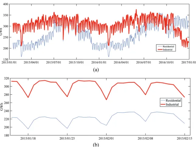
Figs. 2 (a) and (b) show the seasonal effect and time series in real load, which is 2-year period for long term electric load and 1-month period for short term electric load. For 2-year period, it is clearly seen that the effect of seasonality, on the other hand, 1-month period is due to social factors, such as the difference between working days and holidays. It cannot be denied that these factors strongly affect the usage of the electricity.

As a result, 21 inputs composed of weather factors, holiday effect and history load are chosen.

Weather factors include highest, lowest, and average temperature, humidity, and precipitation in Taipei, Taichung and Kaohsiung, hours of daylight which are provided by Central Weather Bureau.

Electricity load pattern for weekday and weekend are different, and load pattern is strongly affected by holiday effect. However, if we use one node such as 1 to 7 to represent a week is not suitable in this case. Aboul-Magd and Ahmed (2001) stated

that the weight of the variable is not related to its numeric value, for example, day 2 (Tuesday) is not twice as important as day 1 (Monday). As a consequence, binary encoding (001 to 111) with three nodes is applied to solve this problem. Taipei, Taichung and Kaohsiung are top electricity usage cities in Taiwan, since electricity usage is closely related to weather conditions, highest, average,

lowest temperature and precipitation are chosen to be the input variables.

The neural network model sometimes is unstable due to the drawbacks of back-propagation including low training speed and easily influenced by noise and weak interdependency data. The problem of overfitting is displayed in Fig. 3.

Overfitting occurs for several reasons, such as too Fig. 2. History long-term load for (a) 2 years (2015.1.1-2016.12.31) and (b) 1 month (2015.1.15-2015.2.15)

(Compiled by the authors)

Fig. 3. Overfitting due to the instability of the model without preprocessing (Compiled by the authors)

many variables or little training data in the model.

To construct a robust neural network model, when best hidden layer neurons are 11, model has the best MAPE (mean absolute percentage error) rate and the least standard deviation by trial and error which is shown in Fig. 4(a). Steepest descent method is commonly used in back-propagation (Liu et al., 2013), but it has a drawback of slower convergence speed. Therefore, updated algorithms were proposed by several scholars (Azadeh et al., 2007; Catalao et al., 2007). Three different algorithms are compared in this paper: gradient descent with momentum and adaptive learning rate backpropagation (GDX), LM backpropagation, and SCG (scaled conjugate gradient). Fig. 4(b) show that LM backpropagation has the best convergence rate and accuracy for prediction which successfully

conquered the disadvantages of steepest descent method, and LM training function can be written as

[J ^TWJ + λdiag(J ^TWJ)]hlm = J ^TW(y ‒ y) (2) where J is Jacobian matrix of derivatives of the residuals with respect to the parameters, λ is damping parameter which is adaptive balance between the 2 steps, W is the weighting matrix, y is the curve-fit function, and hlm is the perturbation of the network. LM algorithm adaptively varies the parameter updates between the gradient descent and the Gauss-Newton update, which accelerate to the local minimum. Therefore, LM as training algorithm is applied in the proposed artificial intelligence model.

Fig. 4. (a) The effect of different hidden layer neurons on the ANN model, then 11 neurons is shown to achieve best MAPE and least standard deviation (b) Comparisons of three algorithms, which are GDX, LM, and SCG (Compiled by the authors)

5. Preprocessing By Rough Set

Systematic solutions are needed to conquer overfitting problem. There are usually two options to select: reducing number of features and regularizing the network. A number of input variables will cause huge computation in ANN model. It is obvious that preprocessing is needed to filter input variables. Therefore, rough set (Affonso et al., 2015) is applied to modify the model since it could handle incomplete, uncertain and ambiguous data containing mass of variables. Rough set is capable of abstracting knowledge or pattern from data, and calculate the significance of each condition attributes and reduce condition attribute with weak data. After eliminating superfluous data, the modified model can enhance its training speed and stability.

In order to effectively eliminate weak interdependency attributes, constructing information and decision table is necessary.

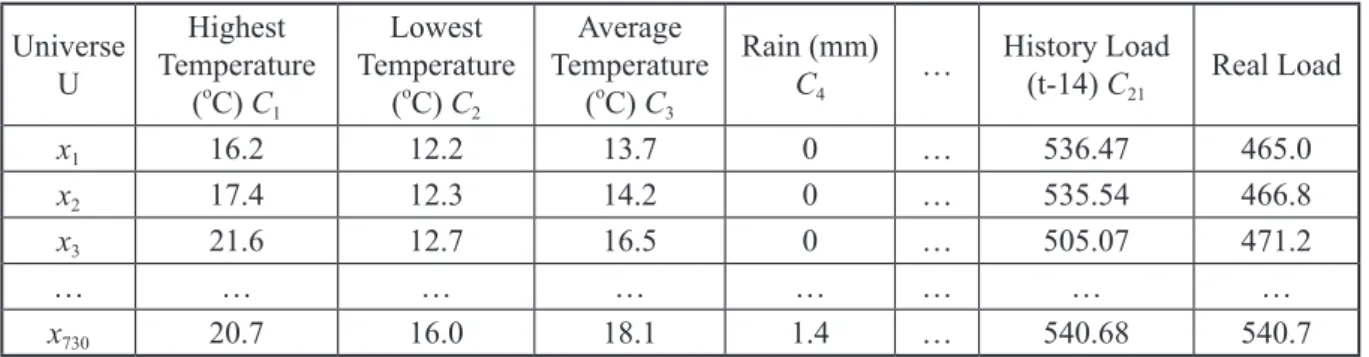
Table 1 shows a part of condition attributes, which are weather factors and holiday effect, and decision attributes is the target load. The process of attribution reduction with rough set is shown as Fig. 5(a). All the data in condition attribute is characterized by equal interval scaling. After analyzing the total load pattern, target total load can be separated by two parts, which are industrial load and residential load. If equal interval scaling

is applied to the target total load, it might not be suitable. From the collected data, it is obvious to see that the different electricity consumption pattern between residential and industrial load. To be more specific, it is necessary to understand the consumption pattern to help have a better power transmission and distribution system. Therefore, a better classification technique is needed. K-means clustering (Azadeh et al., 2012) is applied here to discretize, and it can be written as

(3) where k represents number of clustering, and c is the center of clusters. The aim of this algorithm is to minimize the squared error function, where ||xi( j)

‒ cj ||² is a distance between a data point xi( j) and the cluster centre cj. It indicates the distance of n data points from their respective cluster centres cn. The process of the characteristic for each condition attribution with k-means clustering is shown as Fig. 5(b). After utilizing this method, the characteristic for total load is shown in Fig. 6. The knowledge system and equivalence relationship can be found through classification. To establish an information system, let I = ( , ), where I is information system, is the universe, and is a non-empty finite set of attributes c such that c:

→Vc for every c∈ . Vc is the set of values of c.

If there exists a set B, with any B⊆ , there is an equivalence relation which can be written as

Table 1. Information and decision system (Compiled by the authors) Universe

U

Highest Temperature

(^oC) C1

Lowest Temperature

(^oC) C2

Average Temperature

(^oC) C3

Rain (mm)

C4 … History Load

(t-14) C21 Real Load

x1 16.2 12.2 13.7 0 … 536.47 465.0

x2 17.4 12.3 14.2 0 … 535.54 466.8

x3 21.6 12.7 16.5 0 … 505.07 471.2

… … … …

x730 20.7 16.0 18.1 1.4 … 540.68 540.7

||x_i^{( j)}

k i =1 k

j =1 c_j||²

Fig. 5. The process of (a) attribution reduction with rough set and (b) the characteristic for each condition attribution with k-means clustering (Compiled by the authors)

Fig. 6. Cluster assignments with centroids for load by k-means clustering (Compiled by the authors)

IND(B)={(x, x ̂ )∈ ² |∀c∈B,c(x)=c(x ̂ )} (4) where IND(B) is called the B-indiscernibility relation. If (x, x ̂ )∈IND(B), then object x and x ̂ are indiscernible from each other by attributes from B.

In addition, upper and lower approximation are set up, which can be illustrated as

B(X)={x│[x]B ⊆X} (5)

¯B (X)={x│[x]B ∩X ≠ ∅} (6) where B(X) is lower approximation, ¯B (X) is upper approximation, x is an element of universe and [x]B

is an equivalence class of universe that be divided by B. In this paper, upper approximation means that the attributes may probably affect electricity demand, and lower approximation represent the attributes directly affect electricity demand. In this regard, the knowledge dependency (Pawlak, 1982) can be defined as

(7) where posC(D) is the positive region, which means the set inside the lower approximation of condition C to decision D, and U represents universe.

From this function, the dependency rate from the condition attributes to decision attribute can be easily calculated. If the dependency rate achieved the maximum value, it means that the selected inputs are essential to the electricity demand.

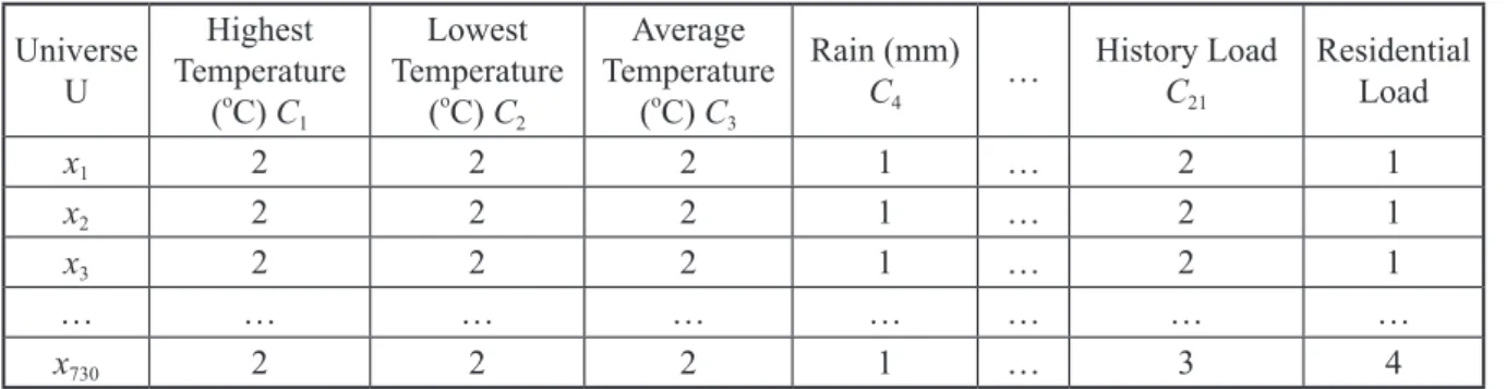
Table 2 shows the information system after characterization, weather data is replaced by equal

interval scaling. With regard to the load data, after applied k-means clustering, each data is replaced with its k-cluster, where k is in the range of 1 to 4. In order to optimize the dependency rate, significance of each condition attribute is employed here. Some attributes are not important than others in a system. Those superfluous data in the information system can be eliminated from the significance analysis in rough set. The significance analysis is similar to Eq. (7). The significance of each attribute a to D is defined by

(8)

γc-(a)(D) is the dependency of condition C without

attribute a to decision D. Significance analysis provides reference to filter unnecessary inputs to electricity demands and further improve the stability of the model to have a better training neural network model.

6. Simulation Result

In this section, the simulation result of preprocessing is displayed, and prediction of two models are compared. Significance analysis is employed to filter insignificant factors. 9 unimportant variables are filtered out to achieve the maximum dependency of 81%, which are average, lowest temperature and rain in Taipei

c(D)= |pos |

|U^c | (D)

Table 2. Information system after characterization (Compiled by the authors) Universe

U

Highest Temperature

(^oC) C1

Lowest Temperature

(^oC) C2

Average Temperature

(^oC) C3

Rain (mm)

C4 … History Load C21

Residential Load

x1 2 2 2 1 … 2 1

x2 2 2 2 1 … 2 1

x3 2 2 2 1 … 2 1

… … … …

x730 2 2 2 1 … 3 4

(C, D)(a) = ^c(D) (D)

c(D)

and Taichung, average and rain in Kaohsiung.

Significance analysis indicates that these factors don’t affect the result much compared to other factors. When 9 factors are deleted, the dependency rate reaches the maximum. After training, the load time series of 12 condition attributes from forecasting samples are used as input vectors in the simulation of the proposed modified model, and the predictions of each goal are obtained. The original ANN model is compared with the modified model.

The modified model by rough set with 12 core inputs, which are humidity and highest temperature in Taipei and Taichung, humidity, highest and lowest temperature in Kaohsiung, holiday effect, hour day light, average rain and history load.

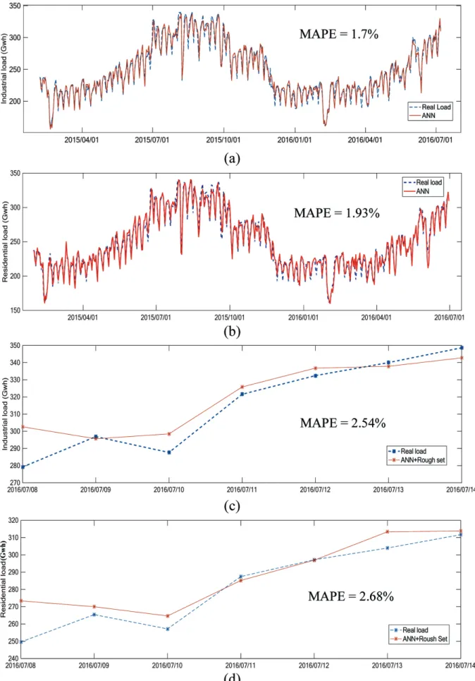
The simulation and prediction results are shown in Fig. 7. The absolute errors between the actual load values and the predictions from ANN and the proposed modified model is shown in Fig. 8.

One ABS error is the absolute error between the actual load value and the predictions on a certain day. The result illustrates that there is only one point at which ANN performs little better than the proposed modified model on 8th July in Fig. 7(c) and one point in Fig. 7(d) where ANN gets a better absolute error on 8th July. Whether the industrial load or the residential load, it is undoubted that the predictions from the proposed modified model are better than those from ANN. On the other hand, the absolute error curve of the proposed modified model passes more points which are better as shown in Figs. 7(c) and (d). With reference to the individuals, the proposed modified model gets 12 better predictions and ANN gets 2 better predictions. And it is obvious that the precision of predictions from the proposed modified model is much better when we take the tendency of the load of a week as a whole one. Moreover, after attribute

elimination, the dependency of condition attribute increase to 81% from 45%. The proposed modified model successfully solved the overfitting problem which occurs frequently for a pure ANN model. By using rough set to eliminate redundant attributes, the modified model has better predictions for one week ahead than pure ANN model.

7. Conclusion

(1) Accurate short-term load forecasting is important nowadays. It is difficult to simulate social factors sensitive to load. The proposed method successfully quantizes social factors such as holiday effect and simulate the load pattern well. All the data collected from Taiwan Power Company and Central Weather Bureau has been tested and validated for short-term load forecasting.

(2) In the training process, LM algorithm is applied to give faster convergence speed and increase the prediction accuracy. The effective number of hidden layer neuron is chosen by trial and error method. The proposed method finds core 12 attributes from 21 attributes for load forecasting. Nine insignificant variables are eliminated by significance analysis of rough set.

In addition, dependency of condition attributes to decision attributes can be improved from 45% to 81%.

(3) The proposed modified model with rough set has been successfully developed for preprocessing, and successfully solves overfitting problem. MAPE of load forecasting with ANN and rough set is within threshold of 3%. The superiority of proposed model is testified with the traditional ANN model.

Fig. 7. Simulation for (a) industrial load and (b) residential load, and prediction for (c) industrial load and (d) residential load by ANN + Rough Set (Compiled by the authors)

Acknowledgments

The authors are grateful to the reviewers for their exceptional efforts in enhancing the style and clarity of this paper. This work was supported by Research Center for Energy Technology and Strategy, National Cheng Kung University, Taiwan, R.O.C.

Reference

Aboul-Magd, M. A. & E. E. E. Ahmed, 2001. An artificial neural network model for electrical daily peak load forecasting with an adjustment for holidays. Power Engineering, 105-113.

Affonso, C., R. J. Sassi & R. M. Barreiros, 2015.

Biological image classification using rough- fuzzy artificial neural network. Expert Systems with Applications, 42(24), 9482- 9488.

Azadeh, A., S. F. Ghaderi, S. Tarverdian, & M.

Saberi, 2007. Integration of artificial neural networks and genetic algorithm to predict electrical energy consumption. Applied Mathematics and Computation, 186(2), 1731- 1741.

Azadeh, A., M. Saberi & Z. Jiryaei, 2012. An intelligent decision support system for

forecasting and optimization of complex personnel attributes in a large bank. Expert Systems with Applications, 39(16), 12358- 12370.

Box, G. E. P. and G.M. Jenkins, 1976. Time series analysis forecasting and control, San Francisco: Holden-Day.

Catalao, J. P. S., S. J. P. S. Mariano & V. Mendes, 2007. Short-term electricity prices forecasting in a competitive market: a neural network approach. Electric Power Systems Research, 77(3), 1297-1304.

Chen, Y., P. B. Luh, C. Guan, Y. Zhao, L.D.

Michel, M. A. Coolbeth, P.B. Friedland,

& S.J. Rourke, 2010. Short-term load forecasting: similar day-based wavelet neural networks. IEEE Transactions on Power Systems, 25(1), 322-330.

Chen, C. J., S. M. Yang & Z. C. Wang, 2012.

Development of a neuro-fuzzy model for airline passenger forecasting. Journal of Aeronautics, Astronautics and Aviation, 44, 169-175.

Do, L. P., K. H. Lin and P. Molnára, 2016.

Electricity consumption modelling: a case of Germany. Economic Modelling, 55, 92-101.

Ekonomou, L., 2010. Greek long-term energy consumption prediction using artificial neural Fig. 8. The comparison of prediction result between the ANN model and the ANN with rough set model

(Compiled by the authors)

networks. Energy, 35, 512-517.

Erdogdu, E., 2007. Electricity demand analysis using cointegration and ARIMA modelling:

a case study of Turkey. Energy Policy, 35, 1129-1146.

Hamzacebi, C., 2007. Forecasting of Turkey's net electricity energy consumption. Energy Policy, 35(3), 2009-2016.

Huang S. J. & K. R. Shih, 2003. Short-term load forecasting via ARIMA model identification including non-Gaussian process considerations. IEEE Transactions on Power Systems, 18(2), 673-679.

Liu, Y. C., S. H. Sun, S. M. Yang & C. Chuang, 2013. Application of genetic algorithm in production scheduling: a case study on the food processing business. Information-An International Interdisciplinary Journal, 15(12), 6063-6075.

Pawlak, Z., 1982. Rough Set. International Journal of Computer & Information Sciences, 11(5), 341-356.

Sarangi, P. K., N. Singh, R.K. Chauhan & R.

Singh, 2009. Short term load forecasting using artificial neural network: a comparison with genetic algorithm implementation. Asian Research Publishing Network Journal of Engineering and Applied Sciences, 4(9), 88- 93.

Sozen, A., Z. Gulseven & E. Arcaklioglu, 2007.

Forecasting based on sectoral energy consumption of GHGs in Turkey and Mitigation policies. Energy Policy, 35(12), 6491-6505.

Su, C. L., S. M. Yang & W. L. Huang, 2011. A two- stage algorithm integrating genetic algorithm and modified newton method for neural network training in engineering systems.

Expert Systems with Applications, 38(10), 12189-12194.

Takeda, H., Y. Tamura & S. Sato, 2016. Using the ensemble kalman filter for electricity load forecasting and analysis. Energy, 104, 184- 198.

Vahidinasab, V., S. Jadid & A. Kazemi, 2008. Day- ahead price forecasting in restructured power systems using artificial neural networks.

Electric Power Systems Research, 78(8), 1332-1342.

Xiao, Z., S. J. Ye, B. Zhong & C. Sun, 2009. BP neural network with rough set for short- term load forecasting. Expert Systems with Applications, 36(1), 273-279.

Yalcinoz T. & U. Yalcinoz, 2005. Short term and medium-term power distribution load forecasting by neural networks. Energy Conversion and Management, 46, 1393-1405.

預處理對類神經網路短期負載動態預測的影響

陳春志

　許倢歆

　游凱為

　楊世銘

摘　要

建立基於粗糙集的短期負載預測類神經網路模型，預測未來一天至一周之電力需求。該模型由 一組數據驗證，包括中央氣象局的天氣因素和台電公司的歷史負載。應用粗糙集通過消除冗餘屬性 來修改模型。預處理的影響提高了類神經網路模型的可靠性，成功地避免了系統的複雜性；因此它

比傳統的類神經網絡模型表現更好。藉由MATLAB模擬預測模型中，發現結果可以提高電力系統預

測的可靠性，進一步幫助能源經濟和策略規劃。

關鍵詞：類神經網路、粗糙集、短期負載預測、預處理

收到日期: 2018年06月11日 修正日期: 2018年11月12日 接受日期: 2018年12月03日

1 長榮大學航運管理學系 副教授

2 國立成功大學能源國際學士學位學程 畢業生

3 國立成功大學航空太空工程學系 教授

*通訊作者電話: 06-2785123#2260, E-mail: [email protected]