Volume 26, No.3, 2021, pp. 127-141 DOI:10.6574/JPRS.202109_26(3).0001
1 Master, Department of Geomatics, National Cheng Kung University Received Date: Apr. 21, 2021
2 Professor, Department of Geomatics, National Cheng Kung University Revised Date: Jul. 05, 2021
* Corresponding Author, E-mail:[email protected] Accepted Date: Aug. 12, 2021
Road Marking Extraction and Classification from Mobile LiDAR Point Clouds Derived Imagery Using Transfer Learning
Miguel Luis R. Lagahit
1 *Yi-Hsing Tseng
2Abstract
High Definition (HD) Maps are highly accurate 3D maps that contain features on or nearby the road that assist with navigation in Autonomous Vehicles (AVs). One of the main challenges when making such maps is the automatic extraction and classification of road markings from mobile mapping data. In this paper, a methodology is proposed to use transfer learning to extract and classify road markings from mobile LiDAR. The data procedure includes preprocessing, training, class extraction and accuracy assessment. Initially, point clouds were filtered and converted to intensity-based images using several grid-cell sizes. Then, it was manually annotated and split to create the training and testing datasets. The training dataset has undergone augmentation before serving as input for evaluating multiple openly available pre-trained neural network models. The models were then applied to the testing dataset and assessed based on their precision, recall, and F1 scores for extraction as well as their error rates for classification. Further processing generated classified point clouds and polygonal vector shapefiles. The results indicate that the best model is the pre-trained U-Net model trained from the intensity-based images with a 5 cm resolution among the other models and training sets that were used. It was able to achieve F1 scores that are comparable with recent work and error rates that are below 15%. However, the classification results are still around two to four times greater than those of recent work and as such, it is recommended to separate the extraction and classification procedures, having a step in between to remove misclassifications.
Keywords: Mobile LiDAR, Road Marking, Extraction, Classification, Transfer Learning
1. Introduction
In recent years, a significant amount of research has been focused on the generation of High Definition (HD) maps. HD Maps are highly accurate three- dimensional (3D) maps that can help an Autonomous Vehicle (AV) navigate on the road. These maps can help an AV precisely localize itself with its surroundings, foresee events beyond the reach of its onboard sensors, and enhance its ability to drive in a complex traffic environment (Liu et al., 2020; Seif & Hu, 2016; Ma et al., 2018). In addition, HD maps also provide an inventory of all stationary assets related to the roadway, including on-road information like road markings and driving lines, and off-road information like traffic signs and roadside vegetation making such maps useful for a wider variety of applications, including urban planning and smart cities, among others (Liu et al., 2020; Ma et al., 2018; Wen et al., 2018).
To create an HD Map, features are extracted from processed sensor data, such as images from cameras and point clouds obtained from LiDAR sensors of Mobile Mapping Systems (MMS). These are positioned using Global Navigation Satellite Systems (GNSSs) and Inertial Measurement Units (IMUs) or
using Simultaneous Localization and Mapping (SLAM) (Liu et al., 2020). In both cases, a huge amount of data is obtained and processed to extract the necessary geometric and semantic information. As such, one of the main challenges in producing an HD Map is achieving full automation (Liu et al., 2020).
An essential component of HD Maps is the vectorized representation of road markings. Road markings are features on the road represented by highly reflective paint such as lane lines, road arrows, and much more, that can serve as warning and guidance for users of the road Ma et al. (2018); Yang et al. (2012);
and Riveiro et al. (2015) used a computer vision technique called intensity thresholding which filters out certain values of intensity to efficiently extract road markings. However, since it only bases on intensity it becomes challenging for complex road environments that represent road markings on varying intensity levels due to different conditions (maintained, fading, etc.).
Kim et al. (2017) on the other hand, used a profile- based intensity analysis that extracts road marking based on road cross-sections. Since cross-sections only represent road markings as lines it becomes difficult for complexly shaped road markings. The inability for both the thresholding and profile-based method to work on complex road markings and road environments gave rise to the alternative use of deep learning for road
marking extraction and classification.
Deep learning has been used on images obtained from cameras onboard vehicles or from MMS to automatically detect and classify road markings. Hoang et al. (2019) made use of a Convolutional Neural Network (CNN) to detect and classify road markings from RGB images obtained from different open datasets. Hu et al. (2019) also made use of a CNN to detect and classify road markings on near-infrared images for night-time applications. However, both image-based methodologies are still sensitive to lighting conditions such as strong sunlight in the morning or weak artificial lighting from lamp posts at night. This greatly affects the capability of the model to successfully detect road markings and correctly classify road markings under such conditions.
This led to the use of deep learning on mobile LiDAR point clouds, which are lighting invariant, for road marking extraction and classification. This is typically done by converting 3D point clouds into intensity-based top-down view 2D images, which is used to train the neural network model. Wolf et al.
(2019) used a U-Net model, a Fully Convolutional Neural Network (FCNN) model, to extract and classify road markings and manhole covers. Wen et al. (2018) took it a step further and developed a deep learning framework, using a modified U-Net model to extract road markings, a CNN for classification after undergoing multi-clustering, and finally, a Conditional Generative Adversarial Network (cGAN) to complete road markings such as broken lines and missing features.
In this work, road markings were automatically extracted and classified from mobile LiDAR point clouds using a deep learning technique called transfer learning. Transfer Learning involves training and making use of pre-trained neural network models.
Initially, the 3D point clouds were filtered and converted to images based on their intensity values.
Then, the images are manually labelled, less than 20%
of which were augmented and used as input for training the pre-trained neural network models. The remainder of the images were used to test the accuracy of the models for road marking extraction and classification.
Finally, the segmented images were either projected back to the point cloud, resulting in a classified point cloud, or converted to polygonal vector shapefiles.
The main contributions of this paper can be summarized as follows: First, multiple openly available pre-trained neural network models available on Supervisely, an online platform for deep learning, were trained and used for both the extraction and classification of road markings. Then, the capabilities of the different models were assessed, this tests the effectiveness of using transfer learning for road marking extraction and classification among the
models that have been used. Second, multiple grid cell sizes were used for converting the 3D point clouds into intensity-based images. This made it possible to investigate the resulting accuracy produced by models trained on different spatial resolutions on the extraction and classification of road markings. Last, a road marking dataset was created, which contained both the labelled and unlabelled intensity images, which was created to encourage further research.
2. Materials and Methods
This part shows the dataset and the methodology.
The proposed methodology is comprised of five main components, namely: data pre-processing, image labeling and data augmentation, transfer learning, inference and assessment, and post-processing of results.
2.1 Test Field and Dataset
Figure 1(a) shows the Shalun test field. It is an area mainly built and developed for AV purposes. It is in Tainan, Taiwan (ROC), and has a total area of around 17,500 square meters. Road markings in this test field are well maintained, meaning that road markings are complete and in good condition. The test field is also enclosed, public vehicles are not allowed to enter the premises and private entities will need proper authentication to enter. This means that there are no other moving or stationary vehicles in the area apart from the mobile mapping unit that could cause occlusions of road markings during the mobile LiDAR scanning.
The point cloud datasets of this test field had an average point density of 10,000 points per square meter, composed of 28 block partitions, and were taken using a RIEGL VMX-250 MMS. It has an IMU, a GNSS receiver, two RIEGL VQ-250 LiDAR scanners, and four cameras (two in front and two at the back). Figure 1(b) shows one of the point cloud block partitions included in the dataset visualized using intensity values.
2.2 Data Pre-Processing
It is necessary to filter the raw point cloud beforehand to retain only ground points. This removes any possible occlusions caused by objects directly above the road markings such as traffic lights, lamp posts, etc. that may cause road markings to be incomplete (e.g., broken lane lines). Ground filtering was implemented using the Point Data Abstraction Library (PDAL Contributors, 2020). First, using the Extended Local Minimum (ELM) method discussed in a study conducted by Chen et al. (2012), low noise points that could potentially affect ground segmentation were identified and removed. Figure 2
shows an example of how ELM works, wherein the differences between all the lowest points in a local area are compared to a defined threshold value, and points exceeding such threshold are removed. In this paper, the ELM used the default parameters, setting the threshold to 1.0 m on a window size of 10.0 m.
(a)
(b)
Figure 1 (a) A top-down ground filtered view of the entire Shalun test field; (b) A sample of one of the point cloud block partitions of the Shalun dataset
Figure 2 The Extended Local Minimum (ELM), taken from Chen et al. (2012)
Then, a Statistical Outlier Removal filter (SOR) was implemented to remove the remaining noise in the point cloud. The SOR works by determining if the mean distance of a point (μ) to several other defined neighboring points is greater than a certain threshold (t).
The threshold (t) is computed using Equation 3, wherein the standard deviation (σ) with respect to the global mean ( ̅) is added to the mean distance of a point (μ) after multiplying by a defined multiplier (m). In this paper, the statistical outlier filter used a default mean distance of 8 nearest neighbors.
̅ = ∑ ... (1)
= ∑ ( − ̅) ... (2)
= + ... (3) Last, the Simple Morphological Filter (SMRF) developed by Pingel et al. (2013) was used to determine the ground points in the point cloud. The SMRF uses an iteration of a series of morphological filters, such as erosion and dilation, until all the points reach a certain threshold difference from the ground points observed from the ELM procedure. Figure 3 shows an example of how the SMRF works. The default parameters that were used for the SMRF were 0.15, 18 meters, 0.5 meters, and 1.25 which are slope, window size, elevation threshold, and elevation scalar, respectively.
Figure 3 The Simple Morphological Filter (SMRF), taken from Pingel et al. (2013)
The ground filtered point clouds were then projected to a planar surface for it to be converted to a top-down view intensity-based 2D image. This was done using a Python implementation of the Geospatial Data Abstraction Library (GDAL/OGR Contributor, 2020). The Inverse Distance Weighting (IDW) method was used to determine the intensity value of a pixel in each grid cell. Equations 4 and 5 shows how IDW estimates an unknown value of a point by using weights derived from the inverses of distances ( ) raised to a defined power (P). In this paper, a default power of 1.0 was used.
( ) = ⋯
⋯ ... (4) ℎ ( ) = ... (5)
Figure 4 show sample results of the ground filtering procedure applied to a block partition. We can see that pole-like objects (e.g., traffic signs, streetlights, etc.) and roadside trees were removed as well as other points that can be considered as noise (e.g., points underground and in the sky).
In this paper, to investigate the effects of different spatial resolutions of LiDAR point cloud derived images, three grid cell sizes were used: 1 cm × 1 cm, 5 cm × 5 cm, and 10 cm × 10 cm in converting the 3D point clouds to intensity-based 2D top-down view images. 1 cm × 1 cm was the smallest grid size that
contains at least one point based on the average point density of the point cloud dataset, and then two increasing intervals of 5 cm were used to obtain two copies of the same image with lower spatial resolution.
Figure 5 shows a sample of a converted intensity-based image on three different grid cell sizes for a block partition.
(a)
(b)
Figure 4 (a) Before and (b) after applying the ground filter procedure
(a)
(b)
(c)
Figure 5 Converted intensity-based images with grid cell size (a) 1 cm × 1 cm, (b) 5 cm × 5 cm, and (c) 10 cm × 10 cm of a block partition of the Shalun dataset
2.3 Image Labelling and Data Augmentation
Image labeling is a procedure where target classifications are identified, and their boundaries are manually traced and defined. Figure 6 shows an example of labeled images taken from Zhou et al.
(2019). In this work, less than 20% of the images were used to train the pre-trained neural network models.
The remaining images were used as ground truth for testing and assessing the accuracy of the models’ results.
Figure 6 Sample images and their labelled counterparts, taken from Zhou et al. (2019)
Data augmentation is a technique used to increase the diversity of a dataset without collecting new data by undergoing image processing methods such as cropping, flipping, rotating, etc. Ho et al. (2019).
Figure 7 shows some visualization of the data augmentation techniques.
Figure 7 Sample visualization of data augmentation techniques, taken from Ho et al. (2019)
Two distinct sets of training images, meaning images found in the first training set are not found in the second training set, were created to be able to test the pre-trained neural network models on all the images.
The specific images used for training are shown in Table 1.
Table 1 Training images used for both sets
Set 1 Image 01 Image 07 Image 18 Image 21 Image 23
Set 2 Image 08 Image 09 Image 13 Image 15 Image 25
Road markings were separated into seven classifications, as shown in Figure 8: longitudinal lines, stop lines, pedestrian crossing, characters, pavement arrows, railroad crossing, and railroad crossing ahead.
“Longitudinal lines” represent the solid and broken lines parallel to the road, such as lane lines or road surface boundaries. “Stop lines” are perpendicular lines that can be found at the end of a road following an intersection that indicates where a vehicle should stop.
“Pedestrian crossing” comprises of consecutive perpendicular lines on the road designated for pedestrians to cross. “Characters” are the numbers and Chinese characters. “Pavement arrows” are directional arrows that show how a vehicle is permitted to move in each lane. “Railroad crossing” is an area on the road marked simulating actual railroad tracks. “Railroad crossing ahead” indicates that a “railroad crossing”
ahead on the road.
(a) (b) (c) (d)
(e) (f) (g)
Figure 8 The 7 road marking classifications and their respective color: (a) longitudinal lines [green];
(b) stop lines[violet]; (c) pedestrian crossing [yellow]; (d) characters [blue]; (e) pavement arrows [cyan]; (f) railroad crossing ahead [red];
and (g) railroad crossing [brown]
Table 2 shows the number of objects per classification per resolution per set. In selecting the
images for training the distribution between the number of objects per class between both sets was considered, having the least differences to remove bias. It can also be seen that the number of objects for most of the classes remains the same throughout the different resolutions ensuring the quality of image annotations.
However, there are cases in which separations between objects become more distinct in higher resolutions and thus increasing the number of objects for that classification, which can be seen in the longitudinal line class.
Table 2 The number of objects per classification per resolution of the original training dataset
Set 1 Set 2
Class 10 cm 5 cm 1 cm 10 cm 5 cm 1 cm
a 55 65 66 53 62 63
b 16 16 16 14 14 14
c 56 56 56 48 48 48
d 2 2 2 4 4 4
e 25 25 25 24 24 25
f 15 15 15 14 14 14
g 1 1 1 1 1 1
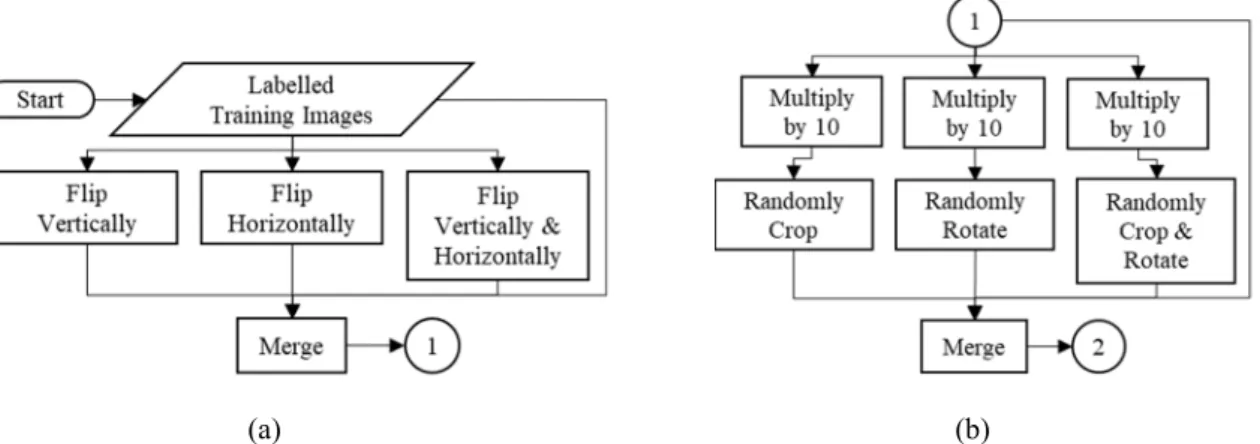
Figures 9 and 10 show the entire augmentation procedure implemented in this research. Initially, copies of the training images were flipped in several directions then merged with the original. Next, copies of the preceding set of images were multiplied and had undergone cropping, rotation, or both and then merged again with the original preceding set of images. Then, the dataset was split in a ratio of 80% and 20%, tagged with “training” for learning and “validation” for checking, respectively. Finally, a background will be added, setting a class for all other unclassified pixels.
In total, an initial training dataset consisting of 5 images increased to 620 images after the data augmentation procedure.
(a) (b)
Figure 9 (a) Part 1 – training images are flipped horizontally, vertically, both, and then merged; (b) Part 2 – training images are cropped, rotated, both, and then merged
(a) (b)
Figure 10 (a) Part 3 – 80% are tagged as “training” and 20% were tagged as “validation”; (b) Part 4 – a background value is added to all unclassified pixels
2.4 Transfer Learning
The concept of transfer learning makes use of a pre-trained neural network model designed for one task and re-training it using a different dataset to apply to another task (Tan et al., 2018). This method speeds up the development of a model by reusing the information stored in its previous training and solves the challenge of having insufficient data in training a model due to the lack of available labeled image datasets (Tan et al., 2018).
Five pre-trained neural network models, which are all openly available on Supervisely, an online platform for deep learning, were trained and used for road marking extraction and classification. A learning rate, batch size, and epoch number of 0.0001, 4, and 20, respectively, were the training parameters used for all of the pre-trained neural network models. A computer with an Intel i7 quad-core processor, 16GB RAM, and an NVIDIA GeForce RTX 1060 graphics card was used to run the model training.
The first model was the U-Net model pre-trained using the ImageNet dataset on a PyTorch framework.
U-Net was originally developed for biomedical image segmentation by the Computer Science Department of the University of Freiburg, Germany (Ronneberger et al., 2015). It is an FCNN, where pooling operations are replaced by upsampling operations (Shelhamer et al., 2017). Figure 11 (a) shows U-Net’s model architecture.
The ImageNet project is a large database built for visual object recognition research which contains more than 14 million labeled images in more than 20,000 categories (Deng et al., 2009).
The second model is the Mask Region- Convolutional Neural Network (R-CNN) model pre- trained using the Microsoft Common Objects in Context (COCO) dataset on a Keras framework. Mask R-CNN is an extension of Faster R-CNN with the addition of a branch for predicting segmentation masks in each region of interest (He et al., 2018). Figure 11 (b) shows Mask R-CNN’s model architecture. The Microsoft COCO dataset is a large-scale dataset, containing more than 300,000 images with 2.5 million instances, that is aimed toward capturing complex everyday scenes of common objects in their natural
context (Lin et al., 2014).
(a)
(b)
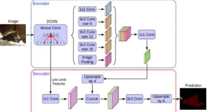
Figure 11 (a) U-Net v2 model architecture, taken from Ronneberger et al. (2015); (b) Mask R-CNN model architecture, taken from He et al. (2018) The third, fourth, and fifth models are DeepLab v3+ models pre-trained using the VOC2012, CityScapes, and ADE20k datasets, respectively, on a TensorFlow framework. DeepLab v3+ is an extension of DeepLabv3 with the addition of a decoder module that improves segmentation results, especially on the boundaries (Chen et al., 2018). Figure 12 shows DeepLab v3+’s model architecture. The VOC2012 dataset is a collection of labelled image datasets built for the PASCAL Visual Object Classes (VOC) Challenge 2012 that was aimed toward providing a standard dataset of images and annotations (Everingham et al., 2012). The CityScapes dataset comprises stereo video sequences recorded in streets from 50 different cities with 5,000 finely annotated images and 20,000 coarsely annotated images (Cordts et al., 2016). The ADE20k dataset is composed of 25,000 annotated images of complex everyday scenes in their natural spatial context (Zhou et al., 2019).
Figure 12 DeepLab v3+ model architecture, taken from Chen et al. (2018)
2.5 Inference and Assessment
The re-trained models were used to infer the remaining mobile LiDAR-derived intensity-based images that were not used for training. Inference outputs a mask that had extracted and classified road markings. In this paper, the extraction procedure is defined as the binary classification between all the road markings and all the other features in the image.
Precision, recall, and F1-score are used to assess the accuracy of the extraction results. This assessment method is widely used in deep learning outputs and was used in the papers of Wen et al. (2018) and Hoang et al.
(2019). The precision was computed using Equation 6.
It is a measure of how many pixels were correctly classified according to the reference image or ground truth. The recall was computed using Equation 7. It is a measure of how many pixels were classified correctly according to the segmented image or predicted results.
The F1 Score is computed using Equation 8. It is the harmonic mean of precision and recall. It is generally used as the final measure of a classification's statistical accuracy.
= ... (6)
= ... (7)
1 = × × ... (8)
The classification procedure is the distinct separation between the different road markings (longitudinal lines, stop lines, etc.). Wen et al. (2018) used Equation 9 to assess the accuracy of their classifications from the separate CNN they used. It is a ratio of the number of erroneous pixels over the number of road marking pixels. Since in this paper, a single neural network model is implemented in both the extraction and classification of road markings, type I and II errors were used. Type I and II errors are error rates like Equation 9 but are specifically based on the
reference image and resulting segmented image, respectively.
= ... (9)
2.6 Post-Processing of Results
Classified point clouds were generated by back projecting the segmented image to the ground filtered point cloud using a Python script. This was done by attaching the classification values of a pixel to their corresponding points. In this paper road marking polygon vector shapefiles were generated from the segmented image and not from the classified point cloud. This procedure was done using the Geospatial Data Abstraction Library (GDAL/OGR Contributors, 2020). Initially, the segmented image was roughly converted to polygons by following the boundaries of pixels that had the same classification values. Polygons with areas less than 10 cm2 were removed and were considered as noise. Then polygon boundaries were simplified by using a tolerance distance value that is the same as the pixel size. Finally, polygons with the same classification values were grouped and merged with all the segmented images in both sets, thus completing the road marking polygon vectors in the entire test field.
Sample attribute information, such as sampling resolution, set number, etc., were included in the shapefiles.
3. Results and Discussion
This part shows the results of the experiment conducted using the proposed methodology for road marking extraction and classification, and its corresponding interpretations based on precision, recall, F1 score, and error rates of the model inferences. This is followed by a discussion in relation to the work of Wen et al. (2018), whose research has involved an extensive assessment of road marking extraction and classification from mobile LiDAR-derived intensity- based images using deep learning. However, in their work, they have used 300 epochs which is far from the 20 epochs that were used in this paper. The number of epochs used here was greatly limited by the processing capability of the available computer. Although, we can see later that results have shown to be comparable and, in some cases, even better considering that there is a huge difference in the number of epochs.
3.1 Resulting Segmented Images
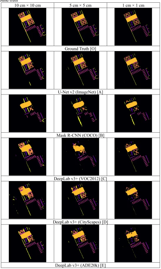
The visualized resulting extractions and classifications of the different pre-trained neural network models at different resolutions as well as the ground truth for one of the block partitions is shown in
Table 3. In terms of pure visual comparison, it is evident that the pre-trained U-Net model at all the resolutions has out-performed the other neural network models when comparing the classification results with
the ground truth. The capital letters found beside the names of the pre-trained neural network models will be used in the succeeding tables to represent road marking extraction and classification results.
Table 3 Sample segmentation results from the different pre-trained models at different image resolutions and the ground truth
10 cm × 10 cm 5 cm × 5 cm 1 cm × 1 cm
Ground Truth [O]
U-Net v2 (ImageNet) [A]
Mask R-CNN (COCO) [B]
DeepLab v3+ (VOC2012) [C]
DeepLab v3+ (CityScapes) [D]
DeepLab v3+ (ADE20k) [E]
3.2 Results of Road Marking Extraction
Tables 4 to 6 show the road marking extraction assessment results for both sets in all the resolutions.
The following results are highlighted in yellow and gray, which indicates the highest and lowest values in a column, respectively.
Table 4 shows the results for precision. It shows how many pixels are classified correctly based on the reference image or ground truth. U-Net had the best precision while Mask-RCNN held the poorest. It was the lowest image resolution, the 10 cm resolution, which had the best precision results.
Table 4 Precision results for all the pre-trained neural network models
Model 10 cm × 10 cm 5 cm × 5 cm 1 cm × 1 cm Set 1 Set 2 Set 1 Set 2 Set 1 Set 2 A 89.97% 88.80% 84.99% 84.45% 85.06% 85.87%
B 60.14% 69.31% 64.47% 67.05% 62.24% 64.25%
C 74.39% 72.96% 70.61% 73.48% 74.98% 72.57%
D 73.59% 77.93% 79.59% 68.60% 72.44% 74.95%
E 78.39% 73.14% 78.10% 69.93% 72.51% 70.62%
Table 5 shows the results for recall. It shows how many pixels are classified correctly based on the segmented image or predicted results. U-Net still held the results. However, unlike precision results, the poorest resulting values were scattered throughout the other models. In this case, it is the 5 cm resolution images that had the best results.
Table 5 Recall results for all the pre-trained neural network models
Model 10 cm × 10 cm 5 cm × 5 cm 1 cm × 1 cm Set 1 Set 2 Set 1 Set 2 Set 1 Set 2 A 78.77% 76.97% 88.39% 86.73% 85.19% 81.44%
B 52.13% 46.83% 49.08% 47.95% 50.39% 47.11%
C 73.01% 64.42% 36.29% 69.41% 59.34% 45.64%
D 64.40% 72.61% 64.88% 61.00% 46.35% 53.70%
E 73.42% 70.60% 68.50% 44.38% 54.38% 35.72%
Table 6 shows the F1 score. It is the harmonic mean of precision and recall. Given that the F1 score considers both the precision and recall, it was interesting to see that the trend of results followed more on recall. The best F1 score came from U-Net, the poorest results were scattered among the other models, and it was the 5 cm resolution images that reflected the best results.
Table 6 F1 score results for all the pre-trained neural network models
Model 10 cm × 10 cm 5 cm × 5 cm 1 cm × 1 cm Set 1 Set 2 Set 1 Set 2 Set 1 Set 2 A 84.00% 82.46% 86.66% 85.57% 85.12% 83.60%
B 55.85% 55.89% 55.73% 55.91% 55.69% 55.85%
C 73.69% 68.42% 47.94% 71.39% 66.25% 56.04%
D 68.69% 75.18% 71.49% 64.58% 56.53% 62.57%
E 75.82% 71.85% 72.99% 54.30% 62.15% 47.44%
Tables 8 to 13 shows the road marking extraction assessment results for both sets in all the resolutions in comparison to the work of Wen et al. (2018). They have used two datasets to evaluate the road marking extraction component of their methodology, a 400 m long road in the TUM-MLS dataset of the Technical University of Munich in Germany, and a highway section from their dataset. They used a modified U-Net model for road marking extraction. They have also tested a cGAN model, a model developed for road marking completion. To evaluate their results, they compared them to the results obtained from implementing traditional computer vision methods used in the papers of Yang et al. (2012); Soilán et al.
(2017), and Cheng et al. (2017).
Table 7 Extraction results of Wen et al. (2018) Model Precision Recall F1-Score
U-Net 70.79% 82.60% 74.42%
cGAN 82.56% 76.48% 79.40%
Others 89.12% 81.31% 85.04%
Wen et al. (2018) using TUM-MLS Dataset U-Net 94.37% 40.24% 56.42%
cGAN 90.15% 82.33% 86.06%
Others 95.97% 87.52% 91.55%
Wen et al. (2018) using their Highway Dataset
Table 7 shows the precision, recall, and F1 score results obtained by Wen et al. (2018) on the TUM-MLS dataset and their dataset, respectively. For simplicity purposes, “U-Net” and “cGAN” represent their results obtained from using those neural network models and
“Others” represents their best results obtained from the traditional computer vision methods. The colors next to the names of each model were used to identify which results were better or equal to theirs in the succeeding tables. This means that if a result is highlighted in that color, they bested the results of that model. In their results, precision and recall obtained through machine learning methods are not always better than those obtained using traditional computer vision. However, F1 score results that consider both precision and recall have shown otherwise.
Tables 8 and 9, show the precision results obtained in the present study as compared to those of Wen et al.
(2018). The pre-trained U-Net model has shown that it could still attain comparable and better results with Wen et al.’s modified U-Net version. Even though the other neural networks have failed to reach the precision of U-Net it was still able to better the resulting precision from traditional computer vision methodologies.
Table 8 Precision results compared to results of Wen et al. (2018) on the TUM-MLS dataset
Model 10 cm × 10 cm 5 cm × 5 cm 1 cm × 1 cm Set 1 Set 2 Set 1 Set 2 Set 1 Set 2 A 89.97% 88.80% 84.99% 84.45% 85.06% 85.87%
B 60.14% 69.31% 64.47% 67.05% 62.24% 64.25%
C 74.39% 72.96% 70.61% 73.48% 74.98% 72.57%
D 73.59% 77.93% 79.59% 68.60% 72.44% 74.95%
E 78.39% 73.14% 78.10% 69.93% 72.51% 70.62%
Table 9 Precision results compared to results of Wen et al. (2018) on their dataset
Model 10 cm × 10 cm 5 cm × 5 cm 1 cm × 1 cm Set 1 Set 2 Set 1 Set 2 Set 1 Set 2 A 89.97% 88.80% 84.99% 84.45% 85.06% 85.87%
B 60.14% 69.31% 64.47% 67.05% 62.24% 64.25%
C 74.39% 72.96% 70.61% 73.48% 74.98% 72.57%
D 73.59% 77.93% 79.59% 68.60% 72.44% 74.95%
E 78.39% 73.14% 78.10% 69.93% 72.51% 70.62%
Tables 10 and 11, show the recall results obtained in the present study as compared to those of Wen et al.
(2018). The U-Net model was still able to show comparable results with that of Wen et al. (2018) and unlike precision, it was evident for both datasets.
Table 10 Recall results compared to results of Wen et al. (2018) on the TUM-MLS dataset
Model 10 cm × 10 cm 5 cm × 5 cm 1 cm × 1 cm Set 1 Set 2 Set 1 Set 2 Set 1 Set 2 A 78.77% 76.97% 88.39% 86.73% 85.19% 81.44%
B 52.13% 46.83% 49.08% 47.95% 50.39% 47.11%
C 73.01% 64.42% 36.29% 69.41% 59.34% 45.64%
D 64.40% 72.61% 64.88% 61.00% 46.35% 53.70%
E 73.42% 70.60% 68.50% 44.38% 54.38% 35.72%
Table 11 Recall results compared to results of Wen et al. (2018) on their dataset
Model 10 cm × 10 cm 5 cm × 5 cm 1 cm × 1 cm Set 1 Set 2 Set 1 Set 2 Set 1 Set 2 A 78.77% 76.97% 88.39% 86.73% 85.19% 81.44%
B 52.13% 46.83% 49.08% 47.95% 50.39% 47.11%
C 73.01% 64.42% 36.29% 69.41% 59.34% 45.64%
D 64.40% 72.61% 64.88% 61.00% 46.35% 53.70%
E 73.42% 70.60% 68.50% 44.38% 54.38% 35.72%
Tables 12 and 13, show the F1 score results obtained in the present study compared to those of Wen et al. (2018). In the end, U-Net was able to provide results that are better or comparable to that of Wen et al. (2018) modified U-Net version. The other models have also shown better results than that of Wen et al.
(2018) results using traditional computer vision methods.
Table 12 F1 score results compared to results of Wen et al. (2018) on the TUM-MLS dataset
Model 10 cm × 10 cm 5 cm × 5 cm 1 cm × 1 cm Set 1 Set 2 Set 1 Set 2 Set 1 Set 2 A 84.00% 82.46% 86.66% 85.57% 85.12% 83.60%
B 55.85% 55.89% 55.73% 55.91% 55.69% 55.85%
C 73.69% 68.42% 47.94% 71.39% 66.25% 56.04%
D 68.69% 75.18% 71.49% 64.58% 56.53% 62.57%
E 75.82% 71.85% 72.99% 54.30% 62.15% 47.44%
Table 13 F1-score results compared to results of Wen et al. (2018) on their dataset
Model 10 cm × 10 cm 5 cm × 5 cm 1 cm × 1 cm Set 1 Set 2 Set 1 Set 2 Set 1 Set 2 A 84.00% 82.46% 86.66% 85.57% 85.12% 83.60%
B 55.85% 55.89% 55.73% 55.91% 55.69% 55.85%
C 73.69% 68.42% 47.94% 71.39% 66.25% 56.04%
D 68.69% 75.18% 71.49% 64.58% 56.53% 62.57%
E 75.82% 71.85% 72.99% 54.30% 62.15% 47.44%
Considering the assessment results, U-Net has shown the best potential for road marking extraction.
The pre-trained U-Net model is up to par with its modified version that is run on significantly more epochs, which also successfully proves the importance of transfer learning in terms of model improvement.
It is also important to take note that the 5 cm resolution had better resulting recall and F1-scores than the 1 cm. This just shows that finer resolutions do not automatically result in better extractions. Higher resolutions might just cause much more noise that could confuse the model. Considering that there are also large differences in file size and image size of the different resolutions, as shown in Table 14, this information can be used to avoid problems in data storage and processing speed. This can also act as a validation that mobile LiDAR point clouds do not have to be that dense, making data acquisition faster and easier.
Table 14 File size and image size of one of the intensity- based images in all the resolutions
10 cm × 10 cm 5 cm × 5 cm 1 cm × 1 cm
File Size (MB) 0.2 0.8 20.0
Image Size
(Pixels) 331 × 339 662 × 636 3305 × 3178
3.3 Results of Road Marking Classification
Tables 15 and 16 show the road marking classification assessment results, the error rate, for both sets in all the resolutions. The error rates that were used are the type I and II errors, which is the ratio between the number of misclassified pixels and the total number of classified pixels based on the reference image and resulting segmented image, respectively. Type I error is complimentary to precision, this means that the trend of results in Table 15 matches with that of Table 4. Type II error is complimentary to recall, this means that the trend of results in Table 16 matches with that of Table 5. The following results are highlighted in yellow and gray, which indicates the highest and lowest values in a column, respectively.
Table 15 Resulting classification Type I error rates Model 10 cm × 10 cm 5 cm × 5 cm 1 cm × 1 cm Set 1 Set 2 Set 1 Set 2 Set 1 Set 2 A 10.03% 11.20% 15.01% 15.55% 14.94% 14.13%
B 39.86% 30.69% 35.53% 32.95% 37.76% 35.75%
C 25.61% 27.04% 29.39% 26.52% 25.02% 27.43%
D 26.41% 22.07% 20.41% 31.40% 27.56% 25.05%
E 21.61% 26.86% 21.90% 30.07% 27.49% 29.38%
Table 16 Resulting classification Type II error rates Model 10 cm × 10 cm 5 cm × 5 cm 1 cm × 1 cm
Set 1 Set 2 Set 1 Set 2 Set 1 Set 2 A 21.23% 23.03% 11.61% 13.27% 14.81% 18.56%
B 47.87% 53.17% 50.92% 52.05% 49.61% 52.89%
C 26.99% 35.58% 63.71% 30.59% 40.66% 54.36%
D 35.60% 27.39% 35.12% 39.00% 53.65% 46.30%
E 26.58% 29.40% 31.50% 55.62% 45.62% 64.28%
U-Net has shown to be the best model by having the least amount of type I and II error in all resolutions.
Here we can still see that lower resolutions have lower error rates, still supporting the fact that higher resolutions do not automatically mean better results.
In the paper of Wen et al. (2018), they have separated extraction from classification. As such, they were able to implement multi-clustering with a set of thresholds in between to further filter-out misclassifications. However, in the case of our methodology, which only involves a single neural network model for both extraction and classification, further steps have been introduced in between.
Table 17 shows the resulting classification error rates of Wen et al. (2018) on three of their datasets: a road section from urban and highway scenarios and an underground garage. They obtained an average of 4.07% with a minimum of 2.41% and a maximum of 6.01%.
Table 17 The classification error rate of Wen et al.
(2018) using their dataset
Urban Highway Underground Average Error Rate 2.41% 6.01% 3.79% 4.07%
Unfortunately, the best results produced error rates around two to four times of Wen et al. (2018), as seen in Tables 15 and 16. Given that the resulting accuracy of extractions produced with the methodology in this paper was on par with theirs, it means that their intermediate procedure of multi-clustering and thresholding greatly improved the classification step. It seems, that in terms of classification it is still better to separate it from the extraction procedure and have an intermediary step that can further remove noise to lower the rate of error. Nonetheless, the pre-trained models of the present study were still able to produce below 15% error rates.
3.4 Post-Processing of Results
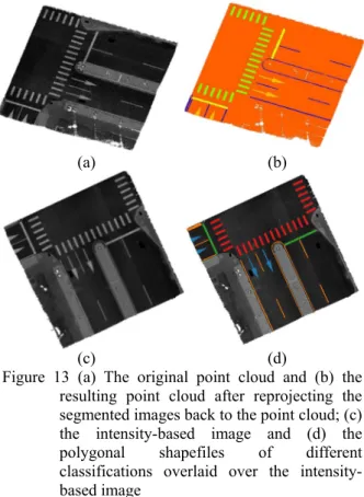
The projection of classification values from the segmented image back to the point cloud was successful. In Figure 13 (Left), the different road and non-road markings from the original point cloud were properly classified. As for the polygonal shapefiles, each classified object was properly converted into individual shapefiles with attributes. In Figure 13 (Right) the shapefiles were properly overlaid over the road markings in the intensity-based images.
(a) (b)
(c) (d)
Figure 13 (a) The original point cloud and (b) the resulting point cloud after reprojecting the segmented images back to the point cloud; (c) the intensity-based image and (d) the polygonal shapefiles of different classifications overlaid over the intensity- based image
A sample of the attribute table of a single pavement arrow polygon is shown in Figure 14. A simple set of information was attached to each object, which includes: (1) “id” a unique number identifier, (2)
“area” the general location or dataset where it can be found, (3) “neuralNetw” the neural network that was used for the extraction and classification, (4) “set” the training set that was used, (5) “samplingRe” the sampling resolution of the images used, and (6) “class”
its classification.
Figure 14 A sample attribute table of one of the polygonal shapefiles of a pavement arrow
4. Conclusions
In this paper, we proposed a methodology that uses transfer learning, a deep learning concept that re- trains and uses pre-trained neural network models, for road marking extraction and classification on mobile LiDAR point cloud-derived intensity-based images.
The extraction results showed that the pre-trained U-Net model had the best potential in road marking extraction having precision, recall, and F1 score results that were better than that of the other pre-trained neural network models that have been used in the study. The pre-trained U-Net model’s extraction results also showed that it is comparable, and in some cases better than, the precision, recall, and F1 score results of Wen et al. (2018), which used a modified version of the U- Net model. This shows that re-training a pre-trained neural network model can produce better results than that of a modified one.
The classification results showed that U-Net still held the best potential. It was able to produce less than 15% type I and II error rates and held the lowest error rate than that of the other pre-trained neural network models used. Unfortunately, in comparison with the error rates of Wen et al. (2018), the error rates obtained in this study were poorer and were around two or four times greater. However, Wen et al. (2018) used a multi- clustering procedure beforehand that eliminated small misclassifications, unlike this work which combined the extraction and classification procedures.
Considering that the extraction results obtained by this study are comparable and better than that of their results, it meant that the multi-clustering procedure has drastically improved their classification. Hence, if semi-automated workflows are to be used, this paper concurs with those of Wen et al. (2018) and recommends that the extraction and classification procedures be separated, with an intermediary step in between to remove unwanted misclassifications.
Although, if the process were to be fully automated, an intermediary step would not be possible and shows the advantage of our method.
In terms of image resolution, the 5 cm × 5 cm resolution obtained better results than the finer 1 cm × 1 cm resolution for both the extraction and classification procedure. This meant that higher spatial resolutions meant better results. As observed in this study, higher resolutions can produce more noise and thus obtain significantly more misclassifications.
Nevertheless, the segmented images were successfully reprojected back to the point cloud, resulting in a classified point cloud, and the segmented images were converted to polygonal vector shapefiles that after some further refinement, can be used for HD Maps.
In future works, other pre-trained models shall be tested as well as other data augmentation techniques and their combinations, to further improve extraction and classification results. Sparse point clouds with the same point density as the grid cell sizes used in image conversion will also be tested. If the results obtained still show that a 5 cm × 5 cm resolution leads to better results than a 1 cm × 1 cm resolution, this will potentially have a huge impact on how mobile LiDAR data is collected, lessening scanning time, and decreasing the output file sizes.
Acknowledgments
This research has been supported and funded by the Ministry of Interior of Taiwan (ROC), under project 109CCL013C.
References
Chen, L.C., Zhu, Y., Papandreou, G., Schroff, F., and Adam, H., 2018. Encoder-decoder with atrous separable convolution for semantic image segmentation, Lecture Notes in Computer Science (Including Subseries Lecture Notes in Artificial Intelligence and Lecture Notes in Bioinformatics), vol. 11211, pp. 833–851.
Chen, Z.Y., Devereux, B., Gao, B.B., and Amable, G., 2012. Upward-fusion urban DTM generating method using airborne Lidar data, ISPRS Journal of Photogrammetry and Remote Sensing, 72: 121–
130.
Cheng, M., Zhang, H., Wang, C., and Li, J., 2017.
Extraction and classification of road markings using mobile laser scanning point clouds, IEEE Journal of Selected Topics in Applied Earth Observations and Remote Sensing, 10(3): 1182–
1196.
Cordts, M., Omran, M., Ramos, S., Rehfeld, T., Enzweiler, M., Benenson, R., Franke, U., Roth, S., and Schiele, B., 2016. The cityscapes dataset for semantic urban scene understanding, in proceedings of the IEEE Computer Society Conference on Computer Vision and Pattern Recognition (CVPR’16), Las Vegas, NV, USA, pp.
3213–3223.
Deng, J., Dong, W., Socher, R., Li, L.J., Li, K., and Fei- Fei, L., 2009. ImageNet: A large-scale hierarchical image database, in proceedings of the IEEE Conference on Computer Vision and Pattern Recognition (CVPR’09), Miami, FL, USA, pp.
248–255.
Everingham, M., Van Gool, L., Williams, C.K.I., Winn, J., and Zisserman, A., 2012. The PASCAL Visual Object Classes Challenge 2012 (VOC2012) Results, Available at: http://www.pascal- network.org/challenges/VOC/voc2012/workshop/
index.html, Accessed March 1, 2020.
GDAL/OGR Contributors, 2020. GDAL/OGR Geospatial Data Abstraction Software Library Library, Available at: https://gdal.org, Accessed March 1, 2020.
He, K., Gkioxari, G., Dollár, P., and Girshick, R., 2018.
Mask R-CNN, IEEE Transactions on Pattern Analysis and Machine Intelligence, 42: 386–397.
Ho, D., Liang, E., and Liaw, R., 2019. 1000x Faster Data Augmentation – The Berkeley Artificial Intelligence Research Blog, Available at:
https://bair.berkeley.edu/blog/2019/06/07/data_au g/, Accessed May 1, 2020.
Hoang, T.M., Nam, S.H., and Park, K.R., 2019.
Enhanced detection and recognition of road markings based on adaptive region of interest and deep learning, IEEE Access, 7: 109817–109832.
Hu, J., Abubakar, S., Liu, S., Dai, X., Yang, G., and Sha, H., 2019. Near-infrared road-marking detection based on a modified faster regional convolutional neural network, Journal of Sensors, 2019:
7174602.
Kim, H., Liu, B., and Myung, H., 2017. Road-feature extraction using point cloud and 3D LiDAR sensor for vehicle localization, in proceedings of the 14th International Conference on Ubiquitous Robots and Ambient Intelligence, South Korea, vol. 2, pp. 891–892.
Lin, Y.T., Maire, M., Belongie, S., Hays, J., Perona, P., Ramanan, D., Dollár, P., and Zitnick, C.L., 2014.
Microsoft COCO: Common objects in context, Lecture Notes in Computer Science (Including Subseries Lecture Notes in Artificial Intelligence
and Lecture Notes in Bioinformatics), vol. 8693, pp.740–755.
Liu, R., Wang, J.L., and Zhang, B.Q., 2020. High definition map for automated driving: Overview and analysis, Journal of Navigation, 73(2): 324–
341.
Ma, L.F., Li, Y., Li, J., Wang, C., Wan, R.S., and Chapman, M.A., 2018. Mobile laser scanned point-clouds for road object detection and extraction: A review, Remote Sensing, 10(10):
1531.
PDAL Contributors, 2020. PDAL - Point Data Abstraction Library — pdal.io. [Online], Available at: https://pdal.io/, Accessed March 1, 2020.
Pingel, T.J., Clarke, K.C., and McBride, W.A., 2013.
An improved simple morphological filter for the terrain classification of airborne LIDAR data, ISPRS Journal of Photogrammetry and Remote Sensing, 77: 21–30.
Riveiro, B., González-Jorge, H., Martínez-Sánchez, J., Díaz-Vilariño, L., and Arias, P., 2015. Automatic detection of zebra crossings from mobile LiDAR data, Optics and Laser Technology, 70: 63–70.
Ronneberger, O., Fischer, P., and Brox, T., 2015. U-net:
Convolutional networks for biomedical image segmentation, Lecture Notes in Computer Science (Including Subseries Lecture Notes in Artificial Intelligence and Lecture Notes in Bioinformatics), vol. 9351, pp. 234–241.
Seif, H.G., and Hu, X.L., 2016. Autonomous driving in the iCity—HD maps as a key challenge of the automotive industry, Engineering, 2(2): 159–162.
Shelhamer, E., Long, J., and Darrell, T., 2017. Fully convolutional networks for semantic segmentation, IEEE Transactions on Pattern Analysis and Machine Intelligence, 39(4): 640–
651.
Soilán, M., Riveiro, B., Martínez-Sánchez, J., and Arias, P., 2017. Segmentation and classification of road markings using MLS data, ISPRS Journal of Photogrammetry and Remote Sensing, 123: 94–
103.
Tan, C., Sun, F., Kong, T., Zhang, W., Yang, C., and Liu, C., 2018. A survey on deep transfer learning, Lecture Notes in Computer Science (Including Subseries Lecture Notes in Artificial Intelligence and Lecture Notes in Bioinformatics), vol. 11141, pp. 270–279.
Wen, C.L., Sun, X.T., Li, J., Wang, C., Guo, Y., and Habib, A., 2018. A deep learning framework for road marking extraction, classification and completion from mobile laser scanning point
clouds, ISPRS Journal of Photogrammetry and Remote Sensing, 147: 178–192.
Wolf, J., Richter, R., Discher, S., and Döllner, J., 2019.
Applicability of neural networks for image classification on object detection in mobile mapping 3D point clouds, International Archives of the Photogrammetry, Remote Sensing & Spatial Information Sciences - ISPRS Archives, 42(4/W15):111–115.
Yang, B.S., Fang, L.N., Li, Q.Q., and Li, J., 2012.
Automated extraction of road markings from mobile LiDAR point clouds, Photogrammetric Engineering and Remote Sensing, 78(4): 331–338.
Zhou, B.L., Zhao, H., Puig, X., Xiao, T., Fidler, S., Barriuso, A., and Torralba, A., 2019. Semantic understanding of scenes through the ADE20K dataset, International Journal of Computer Vision, 127(3): 302–321.
1 國立成功大學測量及空間資訊學系 碩士 收到日期:民國 110 年 04 月 21 日
2 國立成功大學測量及空間資訊學系 教授 修改日期:民國 110 年 07 月 05 日
* 通訊作者, E-mail: [email protected] 接受日期:民國 110 年 08 月 12 日
應用轉移學習從移動式光達點雲影像中萃取並分類 路面標記
賴格陸
1*曾義星
2摘要
高精地圖是輔助自動駕駛車所需的高精度 3D 地圖,目前應用移動式測繪資料自動化測製高精地圖仍 是挑戰,本文提出應用轉移學習 (Transfer Learning) 從移動式光達點雲自動萃取並分類道路標記的方法,
其資料處理流程包括前處理、訓練、萃取分類、及精度評估,前處理是先過濾非路面點雲再將點雲轉換為 網格式的強度值影像。訓練過程是從選取的訓練資料進行手動註釋和拆分,建立訓練和測試數據集,訓練 數據集可採既有的公開資料庫,再利用現有訓練資料擴充。之後運用訓練好的機器學習模型從光達強度 影像中萃取分類路面標記,然後以人工判讀的成果為參考評估測試成果精度,先評估萃取的正確度、錯誤 率、及 F1 指標,進而評估分類的誤差率,最後將分類的點雲向量化。結果顯示,以 5 cm 解析度的光達 強度影像來預訓練 U-Net 模型最好。基於 F1 指標低且誤差率低於 15%,驗證所提方法可成功萃取並分類 道路標記,其測試成效與最近發表的論文成果相當。然而,所提方法之萃取完整度優於所比較的方法,但 分類精度則不如所比較的方法,主要原因是本研究同時進行萃取及分類,而比較的方法則先萃取,進而濾 除雜訊點群後再進行分類。建議未來研究可將萃取和分類過程分開,增加濾除機制,以降低分類誤差率。