國立宜蘭大學土木工程學系（研究所）碩士論文 Department of Civil Engineering National Ilan University Master Thesis

(1)

國立宜蘭大學土木工程學系（研究所）

碩士論文

Department of Civil Engineering National Ilan University

Master Thesis

新誤差評估技術應用於基本解法和邊界元素法

An application of new error estimation technique in the meshless method and boundary element method

指導教授：陳桂鴻博士

Adivisor : Kue-Hong Chen Ph. D.

研究生：陳俊廷撰 Jun-Ting Chen

中華民國 99 年 6 月

(2)

謝誌

短暫的研究生活轉眼即逝，身為指導教授陳桂鴻老師的首位研究生，既感光榮也倍感壓力，特別感謝陳桂鴻老師在我想逃避及放棄時，給予我很大的包容和鼓勵，讓我有勇氣及毅力走完這條艱辛的研究之路；陳桂鴻老師嚴謹和自學的指導方式讓我從懵懂的大學生，慢慢去學會承擔責任，學習自我成長，從失敗中記取教訓和挫折中進步，也感謝老師在我自得意滿時給我打擊，在我灰心喪志時幫我建立信心，因為有老師的教育，

才讓我有機會重新認識自己，進而改善和進步。

也感謝口試委員陳正宗教授，徐文信教授，歐陽慧濤教授對論文的細心閱讀和給與的寶貴意見，讓我能夠從不同角度去看我的研究結果和檢討研究的過程，使得這篇論文更加的完整。

另外要感謝校內的各位老師、學長姐、同學和學弟妹的陪伴及開導，感謝承宗老師的鼓勵和經驗分享，昱錡學長時時補充我專業知識上的不足，也謝謝福來大哥提供我實務工作上的寶貴經驗和訊息，還有感謝同窗啟明一路跟我互相切磋學習，特別感謝的是佳螢學妹，多虧有妳的陪伴，這條研究之路才少了幾分孤寂。

最後感謝的是我的家人在這段時間的包容和督促，因為有你們全力的支持，這本論文才得以成形。

僅以此篇論文獻給我所有要感謝的人

(3)

Figure captions

Fig. 1-1 The frame of this thesis. 5

Fig. 2-1 Flowchart of the systematic error estimation scheme. 24 Fig. 2-2 Problem sketch and source point distribution for the case 1-1 and case 1-2

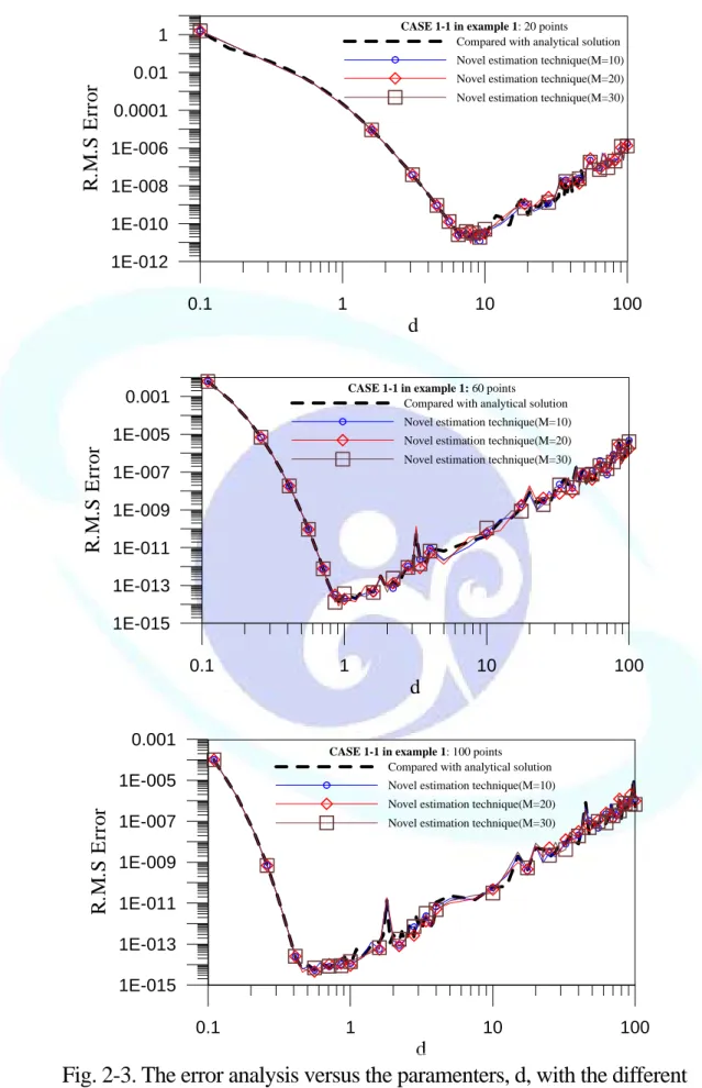
in example 1. (a) two segments (b) four segments. 25 Fig. 2-3 The error analysis for the field solution with the different terms of Trefftz basis

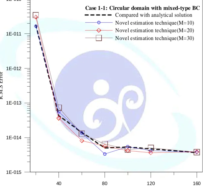
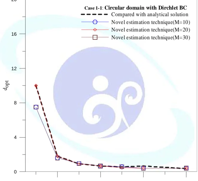
for case 1-1 in example1. (a) 30 points (b) 60 points (c) 100 points. 26 Fig. 2-4 R.M.S error versus the number of nodes for case 1-1 in example1. 27 Fig. 2-5 Convergence curve with optimal parameter for case 1-1 in example1. 28 Fig. 2-6 The error analysis for the field solution with the different terms of Trefftz basis

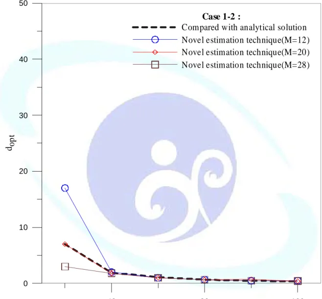
for case 1-2 in example1. (a) 40 points (b) 80 points (c) 120 points. 29 Fig. 2-7 R.M.S error versus the number of nodes for case 1-2 in example1. 30 Fig. 2-8 Convergence curve with optimal parameter for case 1-2 in example1. 31 Fig. 2-9 Problem sketch and source point distribution for the case2-1 in example 1. 32 Fig. 2-10 The error analysis for the field solution with the different terms of Trefftz basis

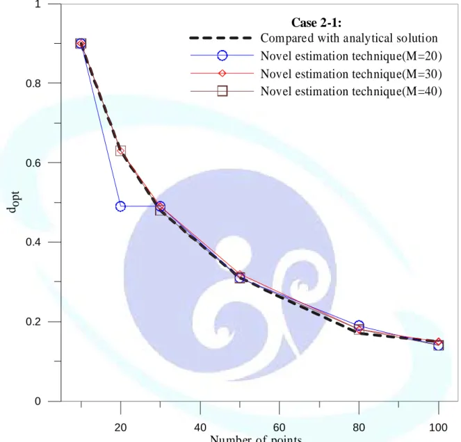
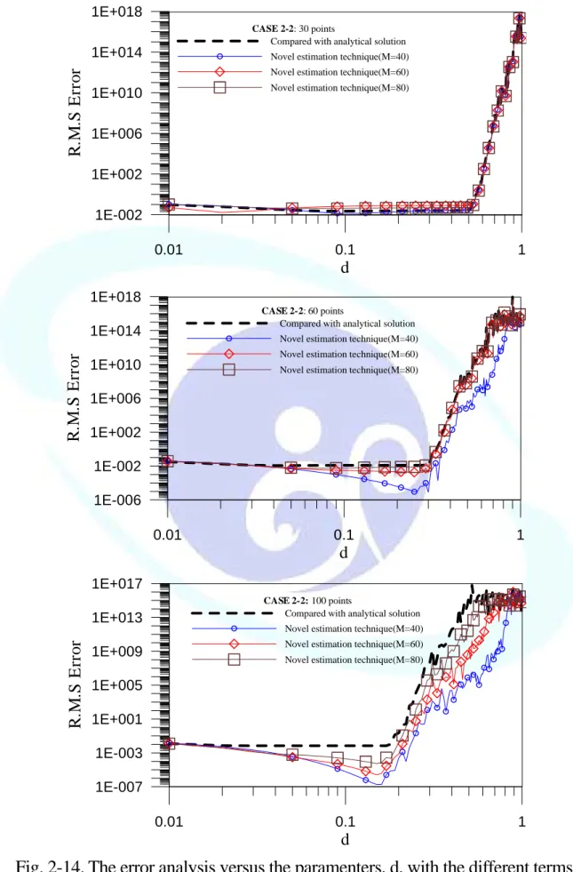
for case 2-1 in example1. (a) 10 points (b) 30 points (c) 80 points. 33 Fig. 2-11 R.M.S error versus the number of nodes for case 2-1 in example1. 34 Fig. 2-12 Convergence curve with optimal parameter for case 2-1 in example 1. 35 Fig. 2-13 Problem sketch and source point distribution for the case2-2 in example 1. 36 Fig. 2-14 The error analysis for the field solution with the different terms of Trefftz basis

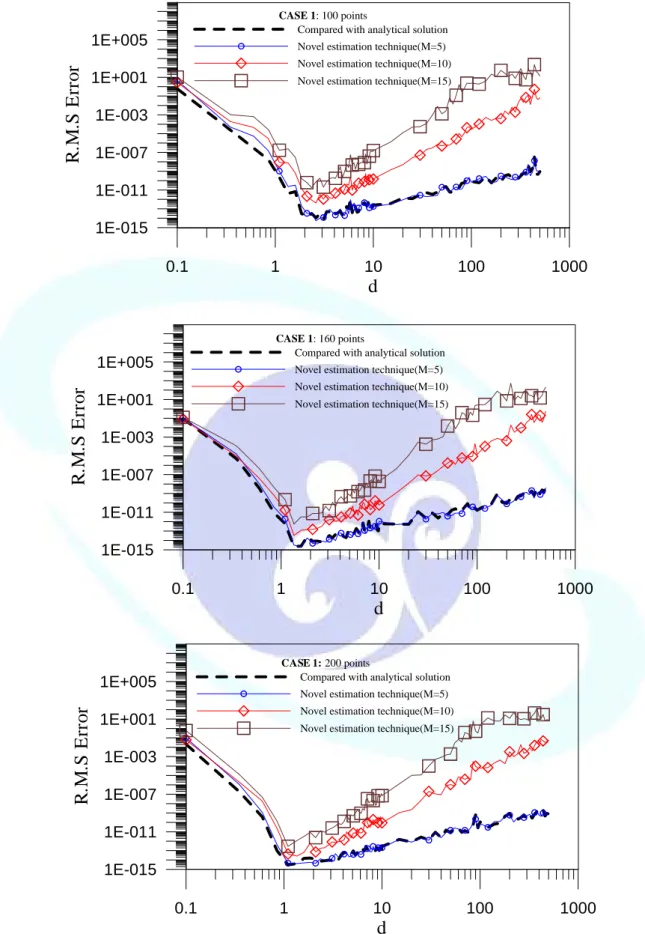
for case 2-2 in example 1. (a) 30 points (b) 60 points (c) 100 points. 37 Fig. 2-15 R.M.S error versus the number of nodes for case 2-2 in example1. 38 Fig. 2-16 Convergence curve with optimal parameter for case 2-2 in example 1. 39 Fig. 2-17 Problem sketch and source point distribution for the case 1 in example 2. 40 Fig. 2-18 The error analysis for the field solution with the different terms of Trefftz basis

(6)

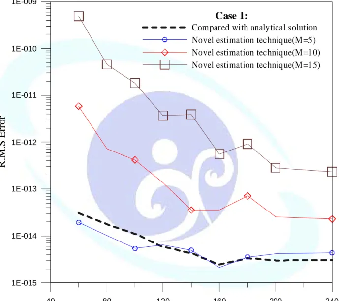
for case 1 in example 2. (a) 100 points (b) 160 points (c) 200 points. 41 Fig. 2-19 R.M.S error versus the number of nodes for case 1 in example 2. 42 Fig. 2-20 Convergence curve with optimal parameter for case 1 in example 2. 43 Fig. 2-21 Problem sketch and source point distribution for the case 2-1 and case 2-2

in example 2. (a) Dirchlet problem (b) Mixed-type problem. 44 Fig. 2-22 The error analysis for the field solution with the different terms of Trefftz basis

for case 2-1 in example 2. (a) 40 points (b) 100 points (c) 160 points. 45 Fig. 2-23 R.M.S error versus the number of nodes for case 2-1 in example 2. 46 Fig. 2-24 Convergence curve with optimal parameter for case 2-1 in example 2. 47 Fig. 2-25 The error analysis for the field solution with the different terms of Trefftz basis

for case 2-2 in example 2. (a) 60 points (b) 100 points (c) 260 points. 48 Fig. 2-26 R.M.S error versus the number of nodes for case 2-2 in example 2. 49 Fig. 2-27 Convergence curve with optimal parameter for case 2-2 in example 2. 50 Fig. 2-28 Problem sketch and source point distribution for the case 3 in example 2. 51 Fig. 2-29 The error analysis for the field solution with the different terms of Trefftz basis

for case 3 in example 2. (a) 40 points (b) 120 points (c) 200 points. 52 Fig. 2-30 R.M.S error versus the number of nodes for case 3 in example 2. 53 Fig. 2-31 Convergence curve with optimal parameter for case 3 in example 2. 54 Fig. 2-32 Problem sketch and source point distribution for the case 1 in example 3. 55 Fig. 2-33 The error analysis for the field solution with the different terms of Trefftz basis

for case 1 in example 3. (a) 100 points (b) 160 points (c) 220 points. 56 Fig. 2-34 R.M.S error versus the number of nodes for case 1 in example 3. 57 Fig. 2-35 Convergence curve with optimal parameter for case 1 in example 3. 58 Fig. 2-36 Problem sketch and source point distribution for the case 2 in example 3. 59 Fig. 2-37 The error analysis for the field solution with the different terms of Trefftz basis

(7)

for case 1 in example 3. (a) 80 points (b) 160 points (c) 200 points. 60 Fig. 2-38 R.M.S error versus the number of nodes for case 2 in example 3. 61 Fig. 2-39 Convergence curve with optimal parameter for case 2 in example 3. 62 Fig. 3-1 Flowchart of the systematic error estimation scheme. 74

Fig. 3-2 Problem sketch for the case 1. 75

Fig. 3-3 The error analysis for the field solution with the different terms of Trefftz

basis for case 1. 76

Fig. 3-4 Convergence rate of computational time with the difference number of elements.

77

Fig. 3-5 Problem sketch for the case 2. 78

basis for case 2. 79

Fig. 3-7 The error analysis for the field solution along the radius ,r=2.43,

with the different number of elements. 80

Fig. 3-8 u (0.248, 0.391) versus number of elements and with the different terms

of Trefftz basis. 81

Fig. 3-9 Problem sketch for the case 3 (a) case 3-1 (b) case 3-2. 82 Fig. 3-10 The error analysis for the field solution with the different terms of Trefftz

basis for case 3-1. 83

basis for case 3-2. 84

(8)

Notations

∇ 2 Laplace operator x Field point s Source point D Interesting domain

) (x

u Potential function of the original problem at the field point x )

(x

t Normal derivative of u(x) at x )

(x

u Boundary potential at the boundary pointx )

(x

t Normal derivative of u(x)at x B Whole boundary

Dirichlet boundary Neumann boundary

n The number of field points

The normal vector at the field point x B1

B2

n x

) (x

φ T-complete set functions Kernel function

Normal derivative of at x

Analytical solution of the new problem at arbitrary point x in the domain M The total number of the T-complete functions

Undetermined coefficient )

, (x s U

) , (x s

L U(x,s)

) (x u^q

vj

) (x

u Boundary potential of the boundary pointxin new problem )

(x

t Normal derivative of u(x)at x

Analytical solution of the original problem u e

)

~ x(

u numerical solution of the new problem Remainder function

R n

(9)

C Bounded constant dopt Optimal parameter

N Number of constant boundary elements )

(x−s

δ Dirac-delta function

Normal derivative of at the boundary point s Normal vector at the boundary point s

) , (x s

T U(x,s)

n s

c~ Undetermined coefficient vector

(10)

Abstract

In order to overcome the drawback of obtaining reliable error estimation the numerical methods in solving realistic engineering problems when an analytical solution is not available, we developed a systematic error estimation scheme in this thesis to estimate the numerical error in the numerical methods without having an analytical solution. In this thesis, a new problem is defined to substitute for the original problem. The governing equation, domain shape and boundary condition type in the new problem are the same as those in the original problem. By adopting the complete Trefftz set as the analytical solution, the analytical solution in the new problem is the known, namely quasi-analytical solution, which is similar with the real analytical solution in the original problem. After implementing numerical methods in the new problem, the error curves can be derived by comparing with the quasi-analytical solution in the new problem. By observing the error curve, we obtained the optimal number of elements or the optimal parameter in the numerical methods at the corner region in the error curve. Therefore, we developed a systematic error estimation scheme in this thesis to estimate the numerical error in the numerical methods. In this thesis, we apply the error estimation technique the boundary element method and the method of fundamental solutions to solve the Laplace problem and several numerical examples are taken to demonstrate the accuracy and efficiency of the proposed estimation technique

Keywords: Trefftz set; quasi-analytical solution; error estimation; optimal number of elements; optimal parameter; method of fundamental solutions; boundary element method;

systematic error estimation scheme.

(11)

摘要

針對實際工程條件很難獲得問題的解析解，本論文發展出一套不用解析解的新誤差評估技術。在本論文中，我們定義了一個新問題去取代原本的問題，這個新問題與原始的問題有著同樣的控制方程、幾何形狀和邊界條件型態，藉由 Trefftz 完全集合函數創造出滿足控制方程式的場解作為解析解，進而定義出一個已知解析解的新問題，新問題的解析解近似於原始問題的解析解；再使用數值方法求解新問題，並與新問題的解析解比較，可求得誤差量，最後獲得收斂的數值結果所需使用的最佳元素數目或最佳參數，因此，本論文成功提出一個系統化的誤差評估技術。最後本論文將此誤差評估技術分別使用在邊界元素法以及基本解法求解二維拉普拉斯問題上，提出數個數值算例，證明本方法在使用上的準確性與有效性。

關鍵詞: Trefftz 集合，模擬解析解，誤差評估，最佳元素數目，最佳參數，基本解法，

邊界元素法，系統化的誤差評估技術。

(12)

Chapter 1 Introduction

1.1 Motivation of the research

In recent years, numerical methods play an important role in solving realistic engineering problems. The numerical method can be utilized to solve the problems governing by PDE equations especially when the exact solution is not easy to obtain. In scientific computing realm of numerical methods, mesh generation of a complicated geometry is always the part of the solution process in the stage of dealing with the problem by implementing numerical method, because those methods require approximations to be made and it’s also the source of error embedded in the numerical methods. The discretization process, which transforms a continuous system into a discrete system with finite number of degrees of freedom, results in errors. The discretization error is defined as the difference between the exact solution and the numerical approximation of the governing equation. However, an exact solution is not easily available in real problem. Obtaining a reliable error estimation is very important in order to guarantee a certain level of accuracy of the numerical result. Thus, the estimation of the discretization error in the numerical methods are worthy of study.

In the Boundary Element Method (BEM), a large number of studies applied the hypersingular equation to find the residual as error estimator [6,11,12], but it cannot be compared in the total error quantity in different number of mesh since it is pointwise error which depends on the number of elements. In meshless methods [13], one way to estimation error is to utilize the residual error, namely posteriori error, the global error magnitude is also unmeaningful to be compared in different number of source points. Wang and his collaborators [30] studied the effect of shape parameters on the numerical accuracy in meshless method. A range of suitable shape parameters is obtained from the analysis of the

(13)

condition number of the system matrix [30]. However, indication of error trend can only been known, but it does not give the error magnitude. The error magnitude has no meaningful to be compared in different number of source points. No matter the numerical methods have require the meshes generation or just only collocation the node points on the boundary, these numerical methods still have some drawbacks that impair their computational ability and even limit their applicability to more practical problems. For this reason, we want to find an objective criterion to compare the total error quantities versus number of meshes or collocation points.

In this thesis, we attempt to establish a novel error estimation technique for detecting the error quantities of the numerical solution including both local error quantity and global error quantity without having analytical solution. The technique give the error magnitude, and the magnitude has meaningful to be compared with different number of elements in the BEM or the shape parameter in the Meshless methods. The optimal number of elements or collocation points, or the optimal shape parameter in numerical methods can be obtained by using the developed novel error estimation technique in unavailable analytic solution condition.

In the error estimation technique, a new problem needs to be defined containing the governing equation, domain shape and boundary condition type. The analytical solution in the new problem, namely quasi-analytical solution, is derived based on the linear combination of the T-complete set which satisfies the same differential equation (DE) operator in the original problem. The quasi-analytical solution similarly to the real analytical solution is simulated to substitute for real analytical solution. After solving the new problem by implementing numerical methods, the error curve can be derived by comparing with the quasi-analytical solution of the new problem. By observing the error curve, we obtained the optimal number of elements or the optimal parameter at the corner region in the error curve. Therefore, we developed a systematic error estimation scheme in this thesis to estimate the numerical error in the numerical methods.

(14)

1.2 Organization of the thesis

The frame of this thesis is shown in Fig. 1-1. In this thesis, the applications of the novel error estimation technique in the method of fundamental solutions (MFS) and BEM are investigated in the context of this thesis. The content of each chapter is summarized below

In chapter 2, the applications of the novel error estimation technique in the MFS for solving Laplace problems with interior, exterior and multiply-connected domain are accomplished. We obtain the optimal parameter in the MFS without having analytical solution by introducing the proposed technique. The accuracy and stability of the proposed technique are verified by the several numerical experiments.

In chapter 3, we extend the novel error estimation technique to the BEM to obtain the optimal number of elements without having analytical solution. Then, the accuracy and stability of the present technique are verified by taking three numerical examples.

Finally, we formulated some conclusions item by item and reveal some further research in the chapter 4.

(15)

Chapter 2

Estimation technique of the optimal parameter for the method of fundamental solutions

Summary

In this thesis, we introduce a novel error estimation technique to obtain the optimal parameter of the method of fundamental solutions (MFS) without having analytical solution.

The convergent numerical solutions of the MFS adopting the optimal parameter can be obtained in unavailable analytical solution condition. This thesis presented a simulated quasi-analytical solution generated by Trefftz basis to substitute for real analytical solution.

The error curve of MFS versus source location parameter can be derived by comparing with the quasi-analytical solution. By observing the error curve versus different parameter, we can obtain the optimal parameter of MFS. Therefore, we develop a systematic error estimation scheme to search for the optimal parameter. By numerical experiments, the optimal parameter in the numerical solutions of the MFS were studied and obtained by using the error estimation technique.

Keywords: error estimation; optimal parameter; method of fundamental solutions; Trefftz set;

quasi-analytical solution

2.1 Introduction

The MFS is a very intuitive meshless technique for obtaining the numerical solution that is attributed to Kupradze and Aleksidze in 1964 [20] and had been applied to a large class of problems, e.g. the potential [26], Helmholtz [23, 27], diffusion, biharmonic problems [28, 33].

(16)

In spite of the fact that, these numerical methods still have some drawbacks that impair their computational ability and even limit their applicability to more practical problems. It is noted that the shape parameter contained plays a very important role in the formulation. In this method a sort of uncertainty principle occurs—we have no criterion to get applicable location of the source points located outside the problem domain. A specific feature of the MFS is to have a wide choice some freedom in choosing the source points. This distance might lead an ill-posed influence matrix, thereby the behavior might lead a solution unstable. We sometimes get the accurate results and sometimes get the poor results when we choose the different sources location.

In order to overcome the above-mentioned drawback, several methods have been reported in the literature [3,4,5,7,9,10,18,19,20,31,32,34-36]. An improved approach called the BKM or BCM was introduced very recently, by Chen and his coworkers [3-5] as well as Kang and his collaborators [18, 19]. The BKM uses the non-singular general solution to avoid the fictitious boundary outside the physical domain in the MFS. The major differences in these meshless methods come only from the techniques used for the chosen non-singular kernels RBFs. In particular, the BKM can produce the symmetric interpolation matrix which is often important in some problems. Another improved method is called the Hybrid boundary node method (Hybrid BNM), which combines the moving least squares (MLS) interpolation scheme with the hybrid displacement variational formulation [35, 36]. However, some integration is still needed as far as with the BNM or Hybrid BNM. The boundary particle method [10] is a truly boundary-only meshfree method for inhomogeneous problems, where the fundamental solution or the general solution is used to evaluate the homogeneous solution, while the high-order fundamental solution of the Laplace operator is employed to calculate the particular solution. The method can produce an accurate result with the boundary nodes for problems whose inhomogeneous function can be represented by a polynomial approximation. It is worth to be mentioned, the method of Novel meshless method (also

(17)

known as the Desingularized meshless method) [7, 9, 31, 32, 34] through using the double-layer potential to regularize the singularity and hypersingularity of the kernel functions and the diagonal terms of influence matrices are easily determined. The source points can be located on the physical boundary, so we don’t confront the problem of the source point distribution.

However, it's a pity that lost the high accuracy with the characteristic of convention MFS.

Even though these methods can locate the source points on the physical boundary and use the non-singular kernels, there still accompanies some difficulty at the ill-posed problems. The success of MFS is due to its excellent performance and high convergence order due to its exponential error convergence rate. From the numerical tests of previous literatures [1, 5, 28, 33], we can found that MFS has good performances regarding accuracy, stability, efficiency, memory requirement, and simplicity of implementation. If the optimal location parameter in the conventional MFS can be detected, the MFS can become a very attractive and dominant numerical method. By adjusting the location parameter, the MFS will gain a highly efficient algorithm that can reach an accuracy that is beyond the reach of the tradition methods. From the theoretically viewpoint, the radius of the enclosing circle, on which the source points of fundamental solutions are distributed, should be increased to as large as possible in the literature [13]. The above mentioned viewpoint for optimal parameter is based on infinite precision computation. In a finite precision computation, the precision is limited to double precision that exist limits for optimal parameter [13]. Therefore, the error estimation technique is needed to determine the optimal parameter. In a real world problem, error is not known because the true solution analytical solution is not given. Without having analytical solution, the optimal parameter cannot be determined. In the literatures [13], one way to estimation error is to utilize the residual error, namely posteriori error. Residual error, which can be obtained a posteriori from the numerical solution without the real analytical solution, has been widely used as an error estimator in adaptive FEM and BEM [11, 12]. However,

(18)

indication of error trend can only been known, but it does not give the error magnitude. The error magnitude has no meaningful to be compared in different number of source points.

In this thesis, we attempt to find an alternative to establish a novel error estimation technique for detecting the optimal parameter in the MFS to obtain the applicable region of the source point distribution without having analytical solution. The technique give the error magnitude, and the magnitude has meaningful to be compared in different number of source points. The convergent solutions of the MFS adopting the optimal distance between the source point and the field point can be obtained in unavailable analytic solution condition. A quasi-analytical solution similarly to the real analytical solution is simulated to substitute for real analytical solution by employing the aid of the Trefftz basis. The error curve can be derived by comparing with the quasi-analytical solution. By observing the error curve, we can obtain the optimal parameter at the corner region of the error curve. Therefore, we develop a systematic error estimation scheme to search for the optimal parameter. The structure of the paper is as follows: In section 2 we review briefly the MFS and the procedure of simulating the new defined problem with the known quasi-analytical solution to put the paper in proper perspectives, and we describe the systematic error estimation scheme in detail. In section 3, we provide numerical of test examples to indicate the validity of the error estimation technique suggested in this paper. We provide a summary and conclusion in section 4.

2.2 Problem statement and method of solution

2.2.1 Problem statement

We consider the behavior of the medium governed by the Laplace equation with the mixed-type boundary conditions (B.C.) as:

∇2u x( )=0,x∈ ∪ ∂D D (2-1)

(19)

), 1

( )

(x u x x B

u = ∈ (2-2)

), 2

) ( ) (

( t x x B

n x x u

t

x

∈

∂ =

= ∂ (2-3)

where is the Laplace operator, is the potential, D is the computational domain of the problem, denotes the whole boundary of the domain D in which of and are the essential boundary (Dirichlet boundary) and natural boundary (Neumann boundary), and is the normal derivative of the potential at x.

∇2 u(x)

D B B1 B

∂ = = ∪

B1

nx 2

(2-4)

B

2

2.2.2 MFS formulation

By employing the radial basis function (RBF) concept, the representation of the solution for interior problem can be approximated in terms of a set of interpolation functions as:

1 1

( ) ( ),

n M

i j j i i

j

u x cφ x x B

=

∑

∈

2 1

( )

( ) ,

i

n j

M

i j i

j x

t x c xv x B

n φ

=

= ∂ ∈

∑

∂ ^(2-5)

for the collocation points, x_i, on the Dirichlet boundary and Neumann boundary, respectively.

j( )xi

φ can be chosen by the fundamental solution of 2D Laplace equation, , shown as follows:

) , (x_i s_j U

( ) ( , ) ln

j xi U x si j rij

φ = = (2-6)

( ) ( , )

( , )

j i i

i j

x x

x U x sj

L x s

n n

φ

∂ ∂

= =

∂ ∂ (2-7)

is the

sj j th source point (singularity), is the th observation point. The N source points are placed outside the domain D.

The potential and its derivative in the normal direction (flux) can be approximated in terms of the linear algebra system as:

xi i

(20)

⎪⎭

⎪⎬

⎫

⎪⎩

⎪⎨

=⎧

⎥⎦

⎢ ⎤

⎣

⎡

) 2 (

) 1 (

2

1 ~

u u U c

U (2-8)

⎪⎭

⎪⎬

⎫

⎪⎩

⎪⎨

=⎧

⎥⎦

⎢ ⎤

⎣

⎡

) 2 (

) 1 (

2

1 ~

t c t L

L (2-9)

After imposing the corresponding boundary conditions, the resulting system of linear equations can be expressed in matrix form of a linear combination of Eq. (2-9) and (2-10) as follows as:

⎪⎭

⎪⎬

⎫

⎪⎩

⎪⎨

=⎧

⎥⎦

⎢ ⎤

⎣

⎡

) 2 (

) 1 (

2

1 ~

t u L c

U

(2-10)

We can derive the unknown coefficient of the linear algebra system in Eq. (2-10) by linear algebraic solver as:

cj

⎪⎭

⎪⎬

⎫

⎪⎩

⎪⎨

⎥ ⎧

⎦

⎢ ⎤

⎣

=⎡

−

) 2 (

) 1 ( 1

2

~ 1

t u L

c U (2-11)

It is noted that the location of source points (shape parameters) have important effect on the accuracy of the MFS and the distance between the fictitious boundary and the physical boundary, defined by d needs to be chosen deliberately. To overcome the abovementioned shortcoming, we develop the estimation technique of optimal parameter to derive the applicable region as shown in Section 3:

2.3 Novel error estimation technique

The derivation in formulating the real analytical solution to gain the error norm in the realistic engineering problem is not obtained easily. To overcome the drawback, an alternative problem is defined. The domain shape and boundary condition type in the new specific problem are the same with the original problem. Furthermore, the analytical solution in the new problem similarly with the real analytical solution in the original problem, namely

(21)

quasi-analytical solution can easily is derived. After solving the new problem by implementing MFS and comparing with the quasi-analytical solution, we develop a novel error estimation scheme in this study. The detail derivation in the novel error estimation technique is presented as:

2.3.1 Definition of new problem

(1). Quasi-analytical solution

In this study, a new boundary-value problem is derived based on the Trefftz basis, this geometry contour and boundary condition type in the new problem are the same with original problem, and also satisfies the same differential equation (DE) operator. The potential, , in the new problem at arbitrary point

) (x u^q xin the domain is the linear combination of the complete set functions as follows:

D x x x

u

M

j j j

q =

∑

∈

=

, ) ( )

(

1

φ

ν (2-12)

)

j(x

φ can be chosen by the T-complete set functions which satisfies the governing Eq.(1), M

is the total number of the T-complete functions andν_jdenotes the undetermined coefficient.

Each of the functions of T-complete set functions satisfies the governing Laplace equation in Eq.(1) as:

[

⁽ ⁾

]

⁰^,

[

⁽ ⁾

]

⁰^, ^,

[

⁽ ⁾

]

⁰^,

[

( )⁽ ⁾

]

⁰

2 )

1 ( 2 )

2 ( 2 )

1 (

2 = ∇ = ∇ = ∇ =

∇ φ x φ x _L φ_M₋ x φ_M x (2-13)

Because of the linear property of differential equation operator in G.E., the potential, satisfies the G.E. as:

) (x u^q ,

[

⁽ ⁾

] [

⁽ ⁾

] [

⁽ ⁾

] [

⁽ ⁾

] [

( )⁽ ⁾

]

⁰

2 )

1 ( 2 1 )

2 ( 2 2 )

1 ( 2 1

2 = ∇ + ∇ + ∇ + ∇ =

∇ u^q x v φ x v φ x _L v_M₋ φ_M₋ x v_M φ_M x (2-14)

The potential, is indeed a analytical solution due to satisfying the G.E. The boundary value in new problem at the M number of collocation points is specified with the boundary

q( ), u x

(22)

condition in the original problem. The boundary value in the new problem is the same with the original problem. The undetermined coefficient,ν , can be determined by matching the _j boundary value on a set of selected points(the M number of points. Therefore, the analytical solution in the new problem is named as the quasi-analytical solution and is similar to the real analytical solution. The two problems have the same boundary contour and boundary condition type, and the boundary conditions of the new problem are given as:

1 1

, ) ( )

(x x x B

u

M

j j

j ∈

=

∑

=

φ

ν _(2-15)

and its derivative in the normal direction (flux) as follows:

2 1

1

, )

j(x )

) ( ) (

( x B

n x n

x x u

t

M

j j M

j x

j j x

∈

∂ =

= ∂

∂

=∂

∑ ∑

=

ω φ ν

(2-16) ν

whereu(x)andt(x)are the known potential and its derivative in the normal direction (flux).

By implementing MFS to solve the new problem, the numerical solution can be compared with the quasi-analytical solution to obtain the error norm.

(2). Error analysis between the new defined problem and the original problem

The relationship between the real analytical solution and quasi-analytical solution are shown as:

( ) ( ) ( )

e q

u x =u x +R xn (2-17)

where

∑

^∞

+

=

1

) ( )

(

M j

j j

n x v x

R φ

The remainder function satisfies the G. E. and it is exponential convergence as

) (x R_n

( ) ( ⁿ), 1

R xn =O r⁻ r> (2-18) Therefore, the difference in the two solver of space is derived as:

u^e( )x −u^q( )x = R_N( )x ≤C r( ⁻^N),

% % (2-19) where C is bounded constant.

(23)

(3). R.M.S comparing with quasi-analytical solution

The error quantity of numerical solution in the new problem adopts the root mean squared (R.M.S) error by comparing numerical solution with quasi-analytical solution, which is defined as follows:

∑

= =

−

= ⁿ

i q n

i

q u

u n n u

S M R

1 2

1

2 1 ( )

/

~ ) 1 ( .

. (2-20)

Where n is the number of field points,u~ x( )is the numerical solution of the new problem by the MFS. The flowchart of the formulation in implementing the novel error estimation scheme is shown in Fig. 2-1.

2.4 Numerical examples

To ensure the accuracy and validity of the error estimation technique to gain the optimal parameter in the MFS, two examples, including different types of geometry shapes and as well as boundary conditions, are solved.

2.4.1 Example 1: Circular domains

In this example, the cross section shown in Fig. 2-2 is circular contour of domain including the interior problems with mixed-type B.C. and exterior problems with Dirichlet discontinuous B.C.s in the cases 1 and 2, respectively.

Case 1: interior problem with mixed-type B.C.s

Case 1-1 and 1-2 are subjected with two and four segments of mixed-type B.C.s as shown in Fig. 2-2(a) and (b), respectively, with corresponding analytical solution given by:

(2-21) Case 1-1: two segments

y e

u^e= ⁰^.⁵^xsin0.5

(24)

In the case, we define the new problem and implementing the MFS to solve it. For the derivation of the optimal parameter, d_opt,

a tained

d

ints fo eter, for dif N

purpose, the R.M.S error by comparing with quasi-analytical solution versus d is plotted for distributing 20, 60, 100 number of source points, respectively, as shown in Fig. 2-3(a)-(c). The new error curve is used as a good indication of error trend, and the error m gnitude approximates to real error. By observing the error curves in Fig. 2-3(a)-(c), the ob optimal parameter is obtained at the corner

of the curves and it approximates to the real tion. To

see the convergent analysis of the MFS, Fig. 2-4 is plotted. A convergent result can be obtained after distributing over 80 po pting the gained by using the new error estimation technique. The optimal param versus number of source point, N, is plotted in Fig. 2-5 to see the variation of N. The ted in investigating the effect of varying N. We see that the aller.

Case 1-2: Four segments

By comparing the numerical solution of new problem with quasi-analytical solution, the R.M.S error versus d is plotted in Fig. 2-6(a)-(c) for distributing 40, 80, 120 points, respectively. By observing the error curves, the obtained optimal parameter is obtained at the corner of the curves. To see the convergent analysis of

convergent result can be obtained after distributing over 80 points. The optimal parameter, versus number of source point, N, is plotted in Fig. 2-8. We see that the N increases an becomes smaller. All numerical conclusions in case1-2 are the same with case1-1.

,d_opt,

compared with the real analytical solu

dop

opt

become

opt

r ado

dopt

f

t

is interes s sm

,

erent increases and

dopt d

dopt

,d_opt,

the MFS, Fig. 2-7 is plotted. A

opt, d

d d_opt

(25)

Case 2: Exterior problems with Dirichlet B.C.s

Case 2-1 and 2-2 are subjected with continuous and discontinuous Dirichlet types of B.C.s as shown in Fig. 2-9 and Fig. 2-13,respectively.

Case 2-1: Continuous B.C.

In this case, the B.C. is specified with θ 4

=cos

u (2-22)

The exact solution is given by:

θ 4 1 cos r4

u= (2-23)

The R.M.S error versus d is plotted in Fig. 2-10(a)-(c) by distributing 10, 30, 80 points, respectively. By observing the error curves, the obtained optimal parameter, is obtained at the corner of the curves. To see the convergent analysis, Fig. 2-11 is plotted. A convergent result can be obtained after distributing over 30 points. The optimal parameter,

opt, d

es and d

opt, d

opt

versus

number of source point, N, is plotted in Fig. 2-12. When N increas becomes smaller. Hence we again observe the good prediction capability of the error estimation scheme.

Case 2-2: Discontinuous B.C.

In this case, the discontinuous B.C. is specified with 1 , 0

(1, )

1 , 2

u θ π

θ π θ π

< <

= ⎨⎧⎩− < <

(2-24) and the analytical solution is derived :

1) ( 2

2tan

2 2 1

−

= ⁻ +

y x u y

π

(2-25)

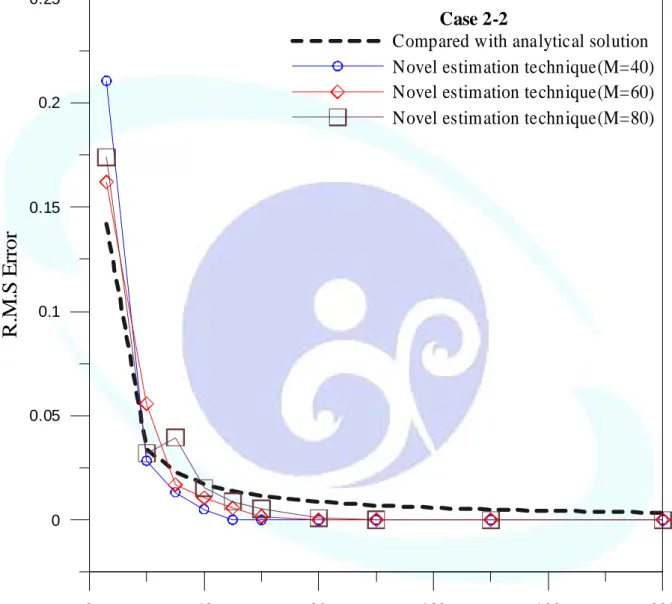
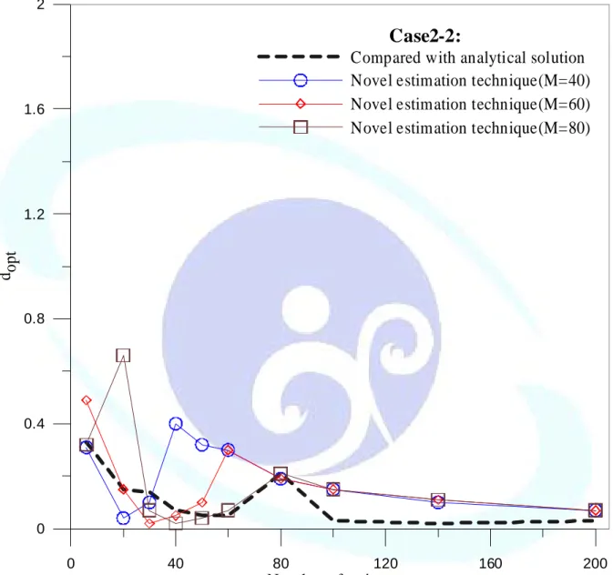
The R.M.S error versus d is plotted in Fig. 2-14(a)-(c) by distributing 40, 60, 80 points, respectively. By observing the error curves, the obtained optimal parameter,d_opt, is obtained

(26)

at the corner of the curves. Fig. 2-15 is plotted to see the convergent effect of MFS by adopting thed_opt.

al param d d_opt

ample 2: arbi

am

n by:

.

at the corner of the curves.

dopt

increases the er

The best convergent result can be obtained after distributing over 40 points.

The optim eter, versus number of source point, N, is plotted in Fig. 2-16. When N increases an becom s similar.

2.4.2 Ex trary domain cases

In this ex ple, the c oss sections in cases 1-3 are more arbitrary contour of domain including th irregular shapes of interesting domain.

Case 1: Peanut shape

Case1 is sub let B.C. as shown in Fig. 2-17, with corresponding analytical solution give

(2-26)

The R.M.S is plotted in Fig. 2-18(a)-(c) by distributing 100, 160, 200 points, respectively By observing the error curves, the obtained optimal parameter is obtained

Fig. 2-19 is plotted to see the convergent effect of MFS by adopting the The best convergent result can be obtained after distributing over 160 points. The optimal param ter, versus number of source point, N

When N and s smaller. Hence we ag

capability of ror e tion scheme.

Case 2: Gear wheel shape

Case 2-1 an bjected with Dirichlet and mixed-type B.C.s as shown in Fig.

2-21(a) and (b), respectively, with corresponding analytical solution given by:

opt, d

e

r

e peanut, gear wheel and

ected with Dirich

d

e

dopt

stima

d 2-2 are su j

error versus

.

θ θ sin 2

2cos

r r

u= +

,d_opt,

, is plotted in Fig. 2-20.

ain observe the good prediction

opt, d

become

(27)

x e

u=3 ¹^.⁵^ycos1.5 ^(2-27)

Case 2-1: Dirichlet B.C.

The R.M.S error versus d is plotted in Fig. 2-22(a)-(c) by distributing 40, 100, 160 points, respectively. By observing the error curves, the obtained optimal parameter is obtained at the corner of the curves. To see the convergent analysis, Fig. 2-23 is plotted. A convergent result can be obtained after distributing over 100 points. The optimal param versus number of source point, N, is plotted in Fig. 2-24. When N increas becomes smaller.

Case 2-2: Mixed type B.C.

The R.M.S error versus d is plotted in Fig. 2-25(a)-(c) by distributing 60, 100, 260 points, respectively. By observing the error curves, the obtained optimal parameter is obtained at the corner of the curves. To see the convergent analysis, Fig. 2-26 is plotted. A convergent result can be obtained after distributing over 100 points. The optimal param versus number of source point, N, is plotted in Fig. 2-27. When N increas becomes smaller.

Case 3: Irregular shape

Case 3 is subjected with Dirichlet B.C. as shown in Fig. 2-28, with having analytical solution as:

(2-28)

The R.M.S error versus d is plotted in Fig. 2-29(a)-(c) by distributing 40, 120, 200 points, respectively. By observing the error curves, the obtained optimal parameter is obtained at the corner of the curves. To see the convergent analysis, Fig. 2-30 is plotted. A convergent

,d_opt,

eter, es and d

opt, d

opt

,d_opt,

eter, es and d

opt, d

opt

y e

u= ⁰^.⁵^xsin0.5

,d_opt,

(28)

result can be obtained after distributing over 120 points. The optimal parameter,d_opt,

opt

ain subjected to

(2-29)

is

opt, d

opt

versus number of source point, N, is plotted in Fig. 2-31. When N increases and becomes smaller.

Therefore, we successfully gain the good prediction once again for mu nnected domain.

2.4.3 Example 3: multiply-connected domain cases

In this example, the potential problems with multiply-connected dom the Dirichlet and mixed-type B.C.s are considered.

Case 1: Dirchlet B.C.

Case 1 is subjected with Dirichlet B.C. as shown in Fig. 2-32, with having analytical solution as:

The R.M.S error versus d is plotted in Fig. 2-33(a)-(c) by distributing 100, 160, 220 points, respectively. By observing the error curves, the obtained optimal parameter obtained at the corner of the curves. To see the convergent analysis, Fig. 2-34 is plotted. A convergent result can be obtained after distributing over 150 points. The optimal param versus

number of source point, N, is plotted in Fig. 2-35. When N increas becomes smaller.

Therefore, we successfully gain the good prediction capability of the error estimation scheme for multiple-connected domain.

Case 2: Mixed-type B.C.

d

ltiple-co

,

ter,

d

y e

u= ^xcos

,d_opt

e es and

(29)

Case 2 is subjected with Mixed-type B.C. as shown in Fig. 2-36, with having analytical solution as:

θ 3

3cos r

u= ^(2-30)

The R.M.S error versus d is plotted in Fig. 2-37(a)-(c) by distributing 80, 160, 200 points, respectively. By observing the error curves, the obtained optimal parameter is obtained at the corner of the curves. To see the convergent analysis, Fig. 2-38 is plotted. A convergent result can be obtained after distributing over 120 points. The optimal param versus number of source point, N, is plotted in Fig. 2-39. When N increas becomes smaller.

Therefore, we successfully gain the good prediction capability of the error estimation scheme for more arbitrary contour of physical domain.

2.5 Concluding remarks

In this thesis, a new estimation technique is developed. We successfully applied the estimation technique in the MFS to derive the optimal parameter without having analytical solution. The technique plays a key role to maintain the system characteristic of MFS due to its excellent performance and high convergence order due to its exponential error convergence rate. The main disadvantage of using MFS which yields the problem in perplexing fictitious boundary can be overcome by the obtained the optimal parameter. The convergent result is found from the convergent study in the cases. Numerical results agreed very well with the analytical solutions. Finally, the several numerical examinations successfully verify the validity of the error estimation technique. We successfully gain the good prediction capability of the error estimation scheme.

,d_opt,

eter, es and d

opt, d

opt

(30)

Chapter 3

An Application of New Error Estimation Technique to the Boundary Element Method

Summary

In this chapter, we develop a novel estimation technique to obtain the optimal number of elements in the boundary element method (BEM) without having analytical solution. A new problem is defined to substitute for the original problem. The governing equation, domain shape and boundary condition type in the new problem are the same as the original problem.

By using the complete Trefftz set as the analytical solution, the analytical solution in the new problem is the known, namely quasi-analytical solution, which is similar with the real analytical solution in the original problem. By implementing the BEM to solve the new problem and comparing with the quasi-analytical solution, the novel error estimation scheme is developed. The error curve of the R.M.S error versus different number of elements can be plotted by the proposed technique. As a result, we can obtain the optimal number of elements in BEM. Several numerical examples are taken to demonstrate the accuracy and efficiency of the proposed estimation technique.

Keywords: Trefftz complete set, boundary element method, estimation technique, quasi-analytical solution

3.1 Introduction

Discretization of the boundary integral equation is an important stage of the BEM in solving engineering problems [2, 6, 11, 13, 17, 21, 29, 38], the discretization process, which transforms a continuous system into a discrete system with finite number of degrees of

(31)

freedom, results in errors. Because of the fact that the reliability of the boundary element approximation is directly related to the discrete boundary element model, in which a proper mesh should be used to represent accurately the original problem both in its geometry and condition. In general, the discretization error is generated from the difference between the exact solution and the numerical result of the governing equation, but the exact solution of engineering problems is difficult to find mathematical formulation out. Furthermore, in the boundary element analysis, number of degrees of freedom depends solely on an analyst’s experience and his/her intuition. Sometime we can get the accurate numerical solution, and sometimes we can get the poor results without having exact solution when we choose the different number of elements. Obviously, the choice of number of elements is a very objective and time-consuming process, and there is no guarantee that the final solution is sufficiently accurate. Obtaining a reliable error estimator is very important in order to guarantee a certain level of accuracy of the numerical result, and is a important ingredient of the stability analysis in numerical methods. Thus, estimation of the discretization error in the BEM is worthy of study.

Different integral equations can be used to find the residual of discretization [6, 13]. A large number of studies applied the hypersingular equation to find the residual as error estimator [6, 13]. Both the singular integral equation UT and hypersingular integral equation LM in the dual BEM can independently determine the unknown boundary data for the problems without a degenerate boundary [6]. The residuals obtained from these two equations can be used as indexes of error estimation. This provides a guide for remeshing without the problem of mismatch of the collocation points on the boundary in the sample point error method.

However, it cannot be compared in the total error quantity in different number of mesh since it is pointwise error which depends on the number of elements. Indication of error trend can only been known, but it does not give the error magnitude. In this thesis, we want to find a way of objective criterion to compare the error quantities in different number of mesh.

(32)

Therefore, we develop the novel error estimator to obtain the optimal number of elements of the BEM without having analytical solution. The convergent numerical solutions of the BEM can be obtained after adopting the optimal number of elements in unavailable analytic solution condition. This study has presented a way of calculating the total error quantity as an asymptotically exact error estimator by implementing the new estimator in BEM based on complete Trefftz set [8, 14, 16, 17, 25, 37] in solving potential problem. A quasi-analytical solution is simulated to substitute for the real analytical solution by employing the aid of the Trefftz set. The convergence analysis of BEM versus different number of elements can be derived in the proposed techniques by comparing with the quasi-analytical solution. By observing the error curve versus different number of mesh, we can obtain the optimal number of elements in BEM. We develop a systematic error estimation scheme to search for the optimal number of elements.

3.2 Problem statement and method of solution

3.2.1 Problem statement

We consider the behavior of the medium governed by the Laplace equation with the mixed-type boundary conditions (B.C.) as:

∇2u(x)= ,0 x∈D (3-1)

), 1

( )

(x u x x B

u = ∈ (3-2)

), 2

) ( ) (

( t x x B

n x x u

t

x

∈

∂ =

= ∂ (3-3)

where is Laplace the operator with problem is the potential, D is the computational domain of the problem

∇2 ,u(x)

,B=B₁∪B₂ =∂D

is the essential boundary (Dirichlet is the natural boundary (Neum

denotes the whole boundary of the domain D, in

which of boundary) in which the potential is

specified, a where the normal derivative of the

B1

B2 nn boundary)

國立宜蘭大學土木工程學系（研究所） 碩士論文 Department of Civil Engineering National Ilan University Master Thesis