電荷可調節特質對粒子沉降及錐形奈米孔道內之離子傳輸行為的影響

doi:10.6342/NTU201801261

國立臺灣大學工學院化學工程學研究所 碩士論文

Graduate Institute of Chemical Engineering College of Engineering

National Taiwan University Master Thesis

電荷可調節特質對粒子沉降及錐形奈米孔道內之離子 傳輸行為的影響

Influence of Charge-Regulated Nature on the Sedimentation of Particle and the Ionic Transport in a

Conical Nanopore

朱育佑 Yu-You Chu

指導教授：徐治平 博士 Advisor: Jyh-Ping Hsu, Ph.D.

中華民國 107 年 7 月 July, 2018

doi:10.6342/NTU201801261

I

中文摘要

在第一章節中，我們研究在電荷可調節的狀況下，粒子沉降受到 其官能基密度、環境 pH 值、鹽濃度以及雷諾數的影響。雷諾數增加

導致越多反離子被拖曳遠離粒子，因此其平均電荷密度下降。粒子越

小會造成電雙層越厚，進而使極化現象更明顯，電荷密度分布更加不

均；球體越小則平均電荷密度越高但所受的電力越小。當粒子夠小

時，其平均電荷密度隨著雷諾數的變化就更加明顯。第二章節探討的

是在電荷可調節的圓錐形奈米孔道中冪次定律流體對離子整流效應所

造成的影響。其考慮的變因有鹽濃度、環境 pH 值、還有冪次定律指

數項時。其離子整流效應在 pH<IEP 以及 pH>IEP 的行為在定性及定

量上都不相同。不同冪次定律指數項

的希對大小隨著鹽濃度呈現極

大的改變。與之相反，離子選擇性則是在 pH<IEP 以及 pH>IEP 的行

為都相似，皆為隨著鹽濃度的增加而有絕對值減少的現象。此選擇性

隨著

的增加而減少。

關鍵字：電荷可調節；沉降；圓錐形奈米孔道；冪次定律流體

doi:10.6342/NTU201801261

II

Abstract

Taking account of the effect of double layer polarization, we first modeled the

sedimentation of a pH-regulated nanoparticle in a generalized field in chapter 1. The

influences of the radius and the density of the functional groups of the particle, the pH and the

bulk salt concentration of the liquid phase, and the Reynolds number Re on the sedimentation

behavior of the particle are examined in detail. We found that as Re increases, because more

counterions are dragged away from the particle surface, its averaged charge density decreases

accordingly. The smaller the particle, the thicker the double layer so that double layer

polarization is more significant and the distribution of the surface charge density is more

nonuniform. Interestingly, the smaller the particle the higher the averaged surface charge

density, but the smaller the electric force acting on it. If the particle is sufficiently large (300

nm in radius), its averaged surface charge density is insensitive to Re as it varies from 0.0025

to 0.04, but can have an appreciable difference (ca. 10 %) if it is small (75 nm).

In chapter 2, we extend previous electrokinetic analyses based on a Newtonian fluid to

power-law fluids, investigating the ion current rectification (ICR) and ion selectivity behaviors

of conical nanopores having a pH-regulated surface. The bulk salt concentration, the solution

pH, and the power-law index n are examined in detail for their influences on these behaviors.

doi:10.6342/NTU201801261

III

We show that the ICR ratio for the case where pH is lower than the isoelectric point (IEP) of

the nanopore surface is different both quantitatively and qualitatively from that for the case

where pH is higher than IEP. The relative magnitude of this ratio as n varies depends largely

on the level of the bulk salt concentration. In contrast, the ion selectivity for pH<IEP is

qualitatively similar to that for pH>IEP, where its absolute value decreases with increasing

bulk salt concentration. In general, this value increases with decreasing n (more non-

Newtonian). Mechanisms are proposed for explaining the observed behaviors in the ICR ratio.

Keywords: Charge regulation; Sedimentation; Conical nanopore; Power law model

doi:10.6342/NTU201801261

IV

Contents

中文摘要 I

English Abstract II

Contents IV

List of Figures V

Chapter 1 Sedimentation of a pH-regulated Nanoparticle in a Generalized

Gravitational Field 1

Reference 15

Chapter 2 Ionic Transport in a pH-Regulated Conical Nanopore Filled

with a Power-law Fluid 38

Reference 51

Conclusion 70

doi:10.6342/NTU201801261

V

List of Figures

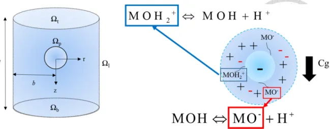
Fig. 1-1. Sedimentation of a rigid, pH-regulated sphere of radius Rp and surface _Ωp

subject to a generalized gravitational field Cg with g being the gravitational

acceleration. For numerical solution purpose, a large cylindrical computation domain of radius b, length l, and surfaces Ω , _t Ω , and _b Ω is defined, and the cylindrical _l

coordinates (r, θ, z) are chosen with the origin at the particle center. ... 19

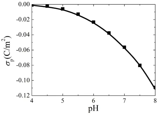
Fig. 1-2. Variation of the surface charge density of an isolated, spherical silica particle

of radius 58 nm in an aqueous KCl solution with pH at Cbulk=100 mM, Nt=2.1 sites/nm²,

pKA=6.38, and pKB=1.87. Discrete symbols: experimental data of Sonnefeld et al.;¹²

curve: present numerical result. ... 20

Fig. 1-3(a). Variation of the scaled electric force (Fe/Fe,ref) acting on a rigid TiO2

particle of radius 300 nm, zeta potential 76.2 mV, and density

ρ

aqueous KCl solution with Cbulk=1.04 10× ⁻³ mM with the reference Reynolds number

Re. Discrete symbols: numerical result of Keller et al.;¹⁴ curve: present numerical

results. ... 21

Fig. 1-3(b). The ratio of the forces (electric force/hydrodynamic force)=(Fe/Fh) on a

rigid TiO2 particle of radius 300 nm, zeta potential 76.2 mV, and density

ρ

kg/m³ in an aqueous KCl solution with Cbulk=1.04 10× ⁻³ mM with the reference

doi:10.6342/NTU201801261

VI

Reynolds number Re. Discrete symbols: numerical result of Keller et al.;¹⁴ curve:

present numerical results. ... 21 Fig. 1-4(a). Variation of the averaged surface charge density σ_Ρ with the bulk salt

concentration Cbulk for various values of Nt at Re=0.01 and pH 8. Curve 1:

7 2

t 5 10 mol/m

N = × ⁻ ; 2: N_t = 7.5 10 mol/m× ^{−7 2}; 3: N_t =10 mol/m^{−6 2}; 4:

6 2

t 1.25 10 mol/m

N = × ⁻ ; 5: N_t =1.5 10 mol/m× ^{−6 2}; 6: N_t = ×2 10 mol/m^{−6 2}.. .. 22

Fig. 1-4(b). The scaled electric force acting on the particle Fe* with the bulk salt

concentration Cbulk for various values of Nt at Re=0.01 and pH 8. Curve 1:

7 2

t 5 10 mol/m

N = × ⁻ ; 2: N_t = 7.5 10 mol/m× ^{−7 2}; 3: N_t =10 mol/m^{−6 2}; 4:

6 2

t 1.25 10 mol/m

N = × ⁻ ; 5: N_t =1.5 10 mol/m× ^{−6 2}; 6: N_t = ×2 10 mol/m^{−6 2}. ... 22

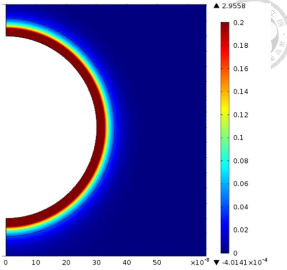
Fig. 1-5. Contours of the concentration difference (CK+- CK+,bulk) (mol/m³) on the half plane

θ=0 at Cbulk=0.1 mol/m³, Re=0.01, pH 8, N_t =10 mol/m^{−6 2}, and Rp=300 nm.

... 23 Fig. 1-6(a). Variation of the averaged surface charge density of a particle σΡ with the

bulk salt concentration Cbulk for various levels of pH at Re=0.01 and

6 2

t 10 mol/m

N = ⁻ . Curve 1: pH 5; 2: pH 5.5; 3: pH 6; 4: pH 7; 5: pH 7.5; 6: pH 8.

... 24 Fig. 1-6(b). The magnitude of the scaled electric force acting on it F_e^* with the bulk

doi:10.6342/NTU201801261

VII

salt concentration Cbulk for various levels of pH at Cbulk=0.1 mol/m³ and

6 2

t 10 mol/m

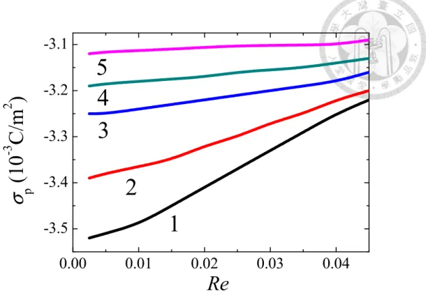
N = ⁻ . Curve 1: pH 5; 2: pH 5.5; 3: pH 6; 4: pH 7; 5: pH 7.5; 6: pH 8.. . 24 Fig. 1-7(a). Variation of the averaged surface charge density σ_Ρ with the Reynolds

number Re for various values of Nt at Cbulk=0.1 mol/m³ and pH 8. Curve 1:

7 2

t 5 10 mol/m

N = × ⁻ ; 2: N_t = 7.5 10 mol/m× ^{−7 2}; 3: N_t =10 mol/m^{−6 2}; 4:

6 2

t 1.25 10 mol/m

N = × ⁻ ; 5: N_t =1.5 10 mol/m× ^{−6 2}; 6: N_t = ×2 10 mol/m^{−6 2}. ... 25

Fig. 1-7(b). The scaled electric force acting on the particle Fe* with the Reynolds

number Re for various values of Nt at Cbulk=0.1 mol/m³ and pH 8. Curve 1:

7 2

t 5 10 mol/m

N = × ⁻ ; 2: N_t = 7.5 10 mol/m× ^{−7 2}; 3: N_t =10 mol/m^{−6 2}; 4:

6 2

t 1.25 10 mol/m

N = × ⁻ ; 5: N_t =1.5 10 mol/m× ^{−6 2}; 6: N_t = ×2 10 mol/m^{−6 2}. ... 25

Fig. 1-8(a). Variation of the averaged surface charge density of a particle σ_Ρ ^{with the}

Reynolds number Re for various levels of pH at Cbulk=0.1 mol/m³ and

6 2

t 10 mol/m

N = ⁻ . ... 26

Fig. 1-8(b). The magnitude of the scaled electric force acting on it F_e^* with the

Reynolds number Re for various levels of pH at Cbulk=0.1 mol/m³ and

6 2

t 10 mol/m

N = ⁻ . Curve 1: pH 5; 2: pH 5.5; 3: pH 6; 4: pH 7; 5: pH 7.5; 6: pH 8. 26

Fig. 1-9. Variation of the percentage difference in the averaged surface charge density

( 0.0025) ( 1)

| | 100%

( 0.0025)

Re Re

D Re

σ σ

Ρ σ Ρ

Ρ

= − =

= ×

= with the bulk salt concentration Cbulk at

doi:10.6342/NTU201801261

VIII

6 2

t 10 mol/m

N = ⁻ , Rp=300 nm and pH 8 ... 27

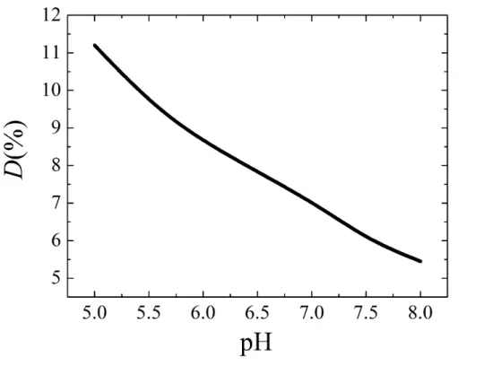
Fig. 1-10. Variation of the percentage difference in the averaged surface charge density

( 0.0025) ( 1)

| | 100%

( 0.0025)

Re Re

D Re

σ σ

Ρ σ Ρ

Ρ

= − =

= ×

= with pH at N_t =10 mol/m^{−6 2}, Rp=300nm and Cbulk=0.1 mol/m³. ... 28 Fig. 1-11. Variation of the surface charge density of a particle σ_Ρ with the Reynolds

number Re for various values of particle radius Rp at Cbulk=0.1 mol/m³,

6 2

t 10 mol/m

N = ⁻ , and pH 8. Curve 1: Rp=75 nm; 2: Rp=100 nm; 3: Rp=150 nm; 4:

Rp=200 nm; 5: Rp=300 nm ... 29

Fig. 1-12(a). Contours of the concentration difference (CK+-CK+

,bulk) (mol/m³) on the half plane θ=0 at Cbulk=0.1mol/m³, Re=0.01, pH 8, Rp=75 nm, and N_t =10 mol/m^{−6 2}

... 30

Fig. 1-12(b). Contours of the concentration difference (CK+-CK+,bulk) (mol/m³) on the half

plane θ=0 at Cbulk=0.1mol/m³, Re=0.01, pH 8, Rp=300 nm, and N_t =10 mol/m^{−6 2}.

... 30

Fig. 1-13. The concentration difference (CK+-CK+

,bulk) (mol/m³) with Re at

Cbulk=0.1mol/m³, pH 8, and N_t =10 mol/m^{−6 2}. Curve 1: Rp=75 nm; 2: Rp=100 nm; 3:

Rp=150 nm; 4: Rp=200 nm; 5: Rp=300 nm. ... 31 Fig. 1-14. Distributions of the surface charge density σ_Ρ along the particle surface

doi:10.6342/NTU201801261

IX

from its south pole (s=0) to its north pole (s=π ) for various levels of R^p at Cbulk=0.1

mol/m³, N_t =10 mol/m^{−6 2}, and pH 8. Curve 1: Rp=75 nm; 2: Rp=100 nm; 3: Rp=150

nm; 4: Rp=200 nm; 5: Rp=300 nm ... 32 Fig. 1-15. Distributions of the surface charge density σ_Ρ along the particle surface

from its south pole (s=0) to its north pole (s=π ) for various levels of Re at

Cbulk=0.1mol/m³, N_t =10 mol/m^{−6 2}, Rp=75 nm, and pH 8 ... 33 Fig. 1-16(a). Variations of the averaged surface charge density of a particle σΡ with

the density of the functional groups N_t for various levels of Re at pH 8 and Cbulk=0.1

mol/m³. ... 34

Fig. 1-16(b). The magnitude of the scaled electric force acting on it Fe* with the density

of the functional groups N_t for various levels of Re at pH 8 and Cbulk=0.1 mol/m³.

Curve 1: Re=0.01; 2: Re=0.02; 3: Re=0.03; 4: Re=0.04. ... 34 Fig. 1-17(a). Variations of the averaged surface charge density of a particle σΡ with

the density of the functional groups N_t for various values of the bulk salt

concentration Cbulk at Re=0.01 and pH 8. Curve 1: Cbulk=0.1 mol/m³; 2: Cbulk=1

mol/m³; 3: Cbulk=5 mol/m³; 4: Cbulk=10 mol/m³. ... 35

Fig. 1-17(b). The scaled electric force acting on it Fe* with the density of the functional groups

Nt for various values of the bulk salt concentration Cbulk at Re=0.01 and pH 8. Curve 1:

doi:10.6342/NTU201801261

X

Cbulk=0.1 mol/m³; 2: Cbulk=1 mol/m³; 3: Cbulk=5 mol/m³; 4: Cbulk=10 mol/m³.

... 35

Fig. 1-18. Variations of the magnitude of the scaled electric force acting on a particle

*

Fe with pH for various levels of Re at N_t =10 mol/m^{−6 2} and Cbulk=0.1 mol/m³. Curve 1: Re=0.01; 2: Re=0.02; 3: Re=0.03; 4: Re=0.04. ... 36 Fig. 1-19. The magnitude of the scaled electric force acting on it F_e^* with pH for

various values of the bulk salt concentration Cbulk at Re=0.01 and N_t =10 mol/m^{−6 2}.

Curve 1: Cbulk=0.01 mol/m³; 2: Cbulk=0.1 mol/m³; 3: Cbulk=1mol/m³; 4: Cbulk=5 mol/m³;

5: Cbulk=10 mol/m³. ... 37

Fig. 2-1. Ionic transport in a pH-regulated conical nanopore of axial length, tip radius,

base radius, and surface charge density, LN, Rt, Rb, and σ_w, respectively, connecting

two large, identical reservoirs. A potential bias V is applied across the nanopore with the

tip end reservoir grounded. (r,θ ,z) are the cylindrical coordinates chosen with its origin

at the nanopore center. The system is filled with a power-law fluid. ... 56

Fig. 2-2. Variation of conductance G with bulk salt concentration for the case of a

conical nanopore of length 1000 nm filled with an aqueous Newtonian KCl solution

with Rt=10 nm, Rb=130 nm, and σ_w^=-0.5e/nm2. Solid lines: approximate result of

Steinbock et al.;³³ discrete symbols: present numerical results. ... 57

doi:10.6342/NTU201801261

XI

Fig. 2-3. Variation in the ionic current rectification factor Rf with the bulk salt

concentration Cbulk for various values of n at pH 7.5. . ... 58

Fig. 2-4(a). Cross-sectional averaged strength of the axial electric field E in a conical

nanopore at pH 7.5, Cbulk=10 mol/m³, V=1 V... ... 59

Fig. 2-4(b). Cross-sectional averaged strength of the axial electric field E in a conical

nanopore at pH 7.5, Cbulk=100 mol/m³, V=1 V. ... 59

Fig. 2-4(c). Axial variation in the cross sectional averaged ionic conductivity Λ in a

conical nanopore at pH 7.5, Cbulk=10 mol/m³, V=-1 V ... 59

Fig. 2-4(d). Axial variation in the cross sectional averaged ionic conductivity Λ in a

conical nanopore at pH 7.5, Cbulk=100 mol/m³, V=-1 V ... 59

Fig. 2-5. Variation in the ionic current rectification factor Rf with the bulk salt

concentration Cbulk for various values of n at pH 4.5 ... 60

Fig. 2-6(a). Axial variation in the cross sectional averaged ionic conductivity Λ at pH

4.5, Cbulk=10 mol/m³, V=1 V. ... 61

Fig. 2-6(b). Axial variation in the cross sectional averaged ionic conductivity Λ at pH

4.5, Cbulk=10 mol/m³, V=-1 V. ... 61

Fig. 2-7(a). Variation in the ion selectivity S with the bulk salt concentration Cbulk for

various combinations of n at V=+1 V, pH 4.5 ... 62

doi:10.6342/NTU201801261

XII

Fig. 2-7(b). Variation in the ion selectivity S with the bulk salt concentration Cbulk for

various combinations of n at V=+1 V, pH 7.5 ... 62

Fig. 2-8. Variation of the ionic current rectification factor Rf with pH for various values

of n at Cbulk=1 mol/m³ ... 63

Fig. 2-9(a). Axial variation in the cross sectional averaged ionic conductivity Λ for

various combinations of n and V at pH 4, Cbulk=1 mol/m³, V=1 V ... 64

Fig. 2-9(b). Axial variation in the cross sectional averaged ionic conductivity Λ for

various combinations of n and V at pH 4, Cbulk=1 mol/m³, V=-1 V ... 64

Fig. 2-10. Axial variation in the cross sectional averaged ionic conductivity Λ for

various combinations of n and V at pH 9, Cbulk=1 mol/m³. (a) V=1 V, (b) V=-1 V ... 65

Fig. 2-11(a). Axial variation in the cross sectional averaged ionic conductivity Λ for

various combinations of n, V, and pH at Cbulk=1 mol/m³, n=0.9, V=1 V ... 66

Fig. 2-11(b). Axial variation in the cross sectional averaged ionic conductivity Λ for

various combinations of n, V, and pH at Cbulk=1 mol/m³, n=0.9, V=-1 V ... 66

Fig. 2-11(c). Axial variation in the cross sectional averaged ionic conductivity Λ for

various combinations of n, V, and pH at Cbulk=1 mol/m³, n=1.0, V=1 V ... 66

Fig. 2-11(d). Axial variation in the cross sectional averaged ionic conductivity Λ for

various combinations of n, V, and pH at Cbulk=1 mol/m³, n=1.0, V=-1 V ... 66

doi:10.6342/NTU201801261

XIII

Fig. 2-12(a). Variation in the ion selectivity S with pH for various combinations of n at

V=+1 V, Cbulk=10 mol/m³ ... 67

Fig. 2-12(b). Variation in the ion selectivity S with pH for various combinations of n at

V=+1 V, Cbulk=1 mol/m³ ... 67

Fig. 2-13(a). Variation in the ionic current contributed by anions, |Ia|, and that by

cations, Ic, at pH 7 for various values of n at Cbulk=10 mol/m³. Red curve: |Ia|; black

curve: Ic. ... 68

Fig. 2-13(b). Variation in the ionic current contributed by anions, |Ia|, and that by

cations, Ic, at pH 5.5 for various values of n at Cbulk=10 mol/m³. Red curve: |Ia|; black

curve: Ic. ... 68

Fig. 2-14(a). Axial variation in the cross sectional averaged concentration of anions at

pH 7 for various values of n at Cbulk=10 mol/m³ ... 69

Fig. 2-14(b). Axial variation in the cross sectional averaged concentration of cations at

pH 5.5 for various values of n at Cbulk=10 mol/m³ ... 69

doi:10.6342/NTU201801261

1

Chapter 1

Sedimentation of a pH-regulated Nanoparticle

in a Generalized Gravitational Field

doi:10.6342/NTU201801261

2

1-1. Introduction

The sedimentation of colloidal particles in an applied field (e.g., gravitational and centrifugal) has been applied to various areas of practical significance, including, for instance, waste water treatment,¹ space propellant recognition, and winemaking.

Applying a molecular dynamics approach, Whitmer et al.² studied the

sedimentation crystallization of colloidal particles; the influences of the gravity, the attractive interaction between aggregating colloids, and their Brownian motion were discussed. They concluded that a moderate level of attractive interaction can enhance the rate of crystallization. Buzzaccaro et al.³ analyzed the sedimentation kinetics of polymeric colloids. Through a novel optical method, they measured the sedimentation profile of dispersions having a very low turbidity. Based on a Stokes approximation and diffusion along the negative gradient of concentration, Song et al.⁴ modeled the sedimentation of particles and colloidal aggregates taking account of streaming. The results obtained explained why suspension having a high particle concentration is more unstable.

The sedimentation behavior of a charged colloidal particle is more complicated than that of an uncharged particle. In the former, the double layer surrounding a particle deforms as it moves, yielding a local electric field which tends to retard its movement. If the particle surface is charge-regulated, its charged conditions are influenced by several factors

doi:10.6342/NTU201801261

3

including, for example, the solution pH and the bulk salt concentration.^{5, 6} The distribution of the surface charge of a particle might also be affected by its movement.⁷

Taking account of counterion condensation and double layer polarization, Bhattacharyya et al.^8-11 evaluated the electric and the hydrodynamic forces acting on a charged, rigid or porous particle as it settles with or without an applied electric field. In the case where an electric field is applied,⁸ they found that the more serious the counterions are dragged away from a particle the more significant the influence of the electric force acting on its behavior.

In a study of the electrokinetic behavior of a charged particle, Sonnefeld et al.¹² found that its surface charge density increases with increasing pH for pH ranging from 4 to 8.

Applying this result, Atalay et al.¹³ analyzed the interaction between a charged nanoparticle and a charged plane. It was found that if the particle is sufficiently close to the plane, the overlapping of their double layers yields an asymmetric distribution in H⁺, resulting in a significant reduction in the surface charge density in the interaction region.

Keller et al.¹⁴ investigated the sedimentation of a rigid sphere having a constant surface potential in a salt solution subject to a generalized gravitational field. It was found that the electric force acting on the particle has a local maximum as Reynolds number varies. This was attributed to the asymmetric distribution of counterions near the particle. Based on a perturbation approach, Keh and Ding¹⁵ derived the dependence of the sedimentation velocity of a rigid sphere having a constant surface charge density in an aqueous, Newtonian salt

doi:10.6342/NTU201801261

4

solution on the thickness of double layer. Taking account of the effect of double layer

relaxation, Yeh et al.¹⁶ modeled the settling of a deformable polyelectrolyte in an unbounded salt solution subject to an applied centrifugal field. The sedimentation behavior of the polyelectrolyte was explained by its effective charge density and the local electric field induced near it. They showed that the sedimentation behavior of a loosely structured polyelectrolyte is dominated by fluid convection. In addition, the shape of a polyelectrolyte is capable of influencing its behavior through affecting the amount of counterions attracted into its interior. Adopting a cell model, Lee et al.¹⁷ analyzed the sedimentation of a

concentrated dispersion of charge-regulated colloidal particles focusing on the effects of the density of the dissociable functional groups on the particle surface, the degree of their dissociation, and the volume fraction of the particle.

In an experimental study of the uptake of gold nanoparticles Cho et al.¹⁸ showed that the amount of uptake depends upon the rate of sedimentation of those particles. Cui et al.¹⁹ demonstrated that the sedimentation and diffusion lead to differences in the degree of association of particles and cells. A decrease in the particle size minimizes the effect of sedimentation on cellular dose or the association of particles and cells. Caruso et al.²⁰ investigated the influence of sedimentation and particle shape on the interaction between cells and particles in a dynamic flow. They showed that this flow minimizes the influence of sedimentation.

doi:10.6342/NTU201801261

5

In this study, the sedimentation of a rigid, pH-regulated sphere in an applied general gravitation field is modeled focusing on the dependence of its velocity on the solution pH, the bulk salt concentration, and the associated Reynolds number. In addition, the variation of the charged conditions of the particle with its sedimentation velocity is examined for the first time. This extends previous studies, where a constant potential/charge density or a uniform charge distribution is almost always assumed.

1-2. Theory

Let us consider the sedimentation of a pH-regulated, isolated spherical particle of radius a and surface Ω in an aqueous salt solution subject to an applied field Cg shown in Figure _p

1-1, where g denotes the gravitational acceleration. For numerical solution purpose, we defined a large cylindrical computation domain of radius b and length l . The cylindrical coordinates (r, θ, z) are adopted with its origin at the particle center. Ω , _t Ω , and _b Ω _l

denote the top, bottom, and lateral surfaces of the computation domain, respectively.

Suppose that the liquid phase is an incompressible fluid and the system is at a pseudo- steady state. If we let

φ

2 4

1 ^{j j}

e j

ρ

φ ε

ε

−∇ = = 

doi:10.6342/NTU201801261

6

4

1

2 ( _{j j})

j

p Fz C

μ φ

=

∇ −∇ −^u



0

∇⋅ = u

0, 1, 2, 3, 4

j j

∇⋅ =

=

(

)

j j j j j

C D C D Fz C

RT

φ

∇⋅ =∇⋅

− ∇ − ∇

Here, ∇ , ∇², j,

ρ

temperature, respectively. zj, Cj, Nj, and Dj are the valence, the molar concentration, the flux, and the diffusivity of ionic species j, respectively.

For convenience, the Reynolds number is defined as Re=2R U_Pρ _ref /μ, where

2

ref 2 P ( - )p / 9

U = R ρ ρ Cg μ is the terminal velocity based on Stokes’ law with

ρ

being the particle density and the magnitude of g, respectively.

The particle surface bears functional groups MOH of surface densities Nt capable of undergoing the following dissociation/association reactions:

MOH ⇔ MO-+H⁺ (6)

MOH2⁺ ⇔ MOH H+ ⁺ (7)

The corresponding equilibrium constants are KA = NMO-[H ]⁺ _S NMOH and

+

B MOH[H ]S MOH2

K =N ⁺ N , where [H ]⁺ _S (mol/m³) is the molar concentration of H⁺ on the

doi:10.6342/NTU201801261

7

surface. Because

t MO

+

N = N

N + N

(C/m²), is

2 B

S A

t

A S S B

[H ] /

[H ] [H ] /

K K

FN K K

σ_Ρ ^ ⁺ ₊ ⁻₊ ^

 

= + + (8)

For the case where the solution pH is adjusted by HCl and KOH the following conditions must satisfy: [H ]⁺ ₀ =10^−pH+3, [OH ]⁻ ₀ =10^{−(14 pH)+3−} , [K ]⁺ ₀ =C_bulk, and

pH+3 (14 pH)+3

0 bulk

[Cl ]⁻ =C +10⁻ −10^{− −} for pH<7; [H ]⁺ ₀ =10^−pH+3, [OH ]⁻ ₀ =10^{−(14 pH)+3−} ,

(14 pH)+3 pH+3

0 bulk

[K ]⁺ =C +10^{− −} −10⁻ , and [Cl ]⁻ ₀ =C_bulk for pH>7. The square brackets denote the molar concentration of a species and the subscript the bulk value.

Suppose that the electric potential and the pressure at a point sufficiently far away from the particle are uninfluenced by the particle. Therefore,

σp

ϕ ε

⋅∇ = −

n on _Ωp (9)

⋅ j =0

n N on _Ωp and Ω _l (10)

φ

0

j j

C =C on Ω , _t Ω , and b Ω l (12)

ref z

= −U

u e on Ω _l (13)

n is the unit outer normal vector of _Ωp, Cj the ionic concentration, and e the unit vector _z

in the z direction.

COMSOL MulitiPhysics (version 4.3a, www.comsol.com) is adopted to solve the present problem numerically. Mesh independence is checked to ensure that the results

doi:10.6342/NTU201801261

8

obtained are reliable and sufficiently accurate. Usually, using ca. 200,000 mesh elements is appropriate.

1-3. Results and discussion

1-3.1 Model verification

To verify the applicability of the solution procedure adopted, we first simulate the variation of the surface charge density of an isolated, spherical silica of Rp=58 nm with pH.

The result shown in Figure 1-2 indicates that the surface charge density increases with increasing pH, and the quantitative values agree well with the experimental data reported by Sonnefeld et al.¹²

The second example is the sedimentation of an isolated rigid TiO2 particle in an aqueous KCl solution solved numerically by Keller et al. Figure 1-3 summarizes the variation of the scaled electric force (Fe/Fe,ref) acting on the particle and the ratio of the forces (electric force/hydrodynamic force)=(Fe/Fh) with the reference Reynolds number Re. Discrete

symbols: numerical result of Keller et al.; curve: present numerical results. As can be seen in this figure, our model is capable of describing the behavior of both (Fe/Fe,ref) and (Fe/Fh).

1-3.2 Numerical Simulation

To examine the behavior of the particle under various conditions, a numerical simulation

doi:10.6342/NTU201801261

9

is conducted by varying its functional group density, the solution pH, the bulk salt

concentration, and the Reynolds number, which is regulated by the applied external field.

For illustration, we assume b=7500 nm and l=15000 nm. We consider a TiO2 particle with Rp=300 nm,

ρ

8.91 10 4

μ = × ⁻ kg/ms, and F=96485 C/mol. For convenience, we define the scaled electric force acting on the particle

F

= F F

/

= εφ

1-3.3Influence of Bulk Salt Concentration

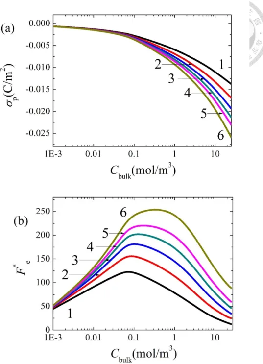
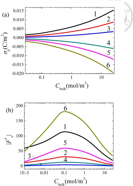
The influence of the density of the functional group of the particle, Nt, on its averaged surface charge density, σΡ, and that on the scaled electric force acting on it, Fe*, at pH 8 are

presented in Figure 4. Since the isoelectric point of the pointis 6.375, the particle is

negatively charged in this case. Figure 1-4 reveals that the larger the Nt the higher the σΡ,

which is expected because the larger the Nt the more amount of ions can be dissociated. Note that Fe* has a local maximum as Cbulk varies. For N_t = ×2 10 mol/m^{−6 2} this local

maximum occurs at Cbulk

≅

≅

doi:10.6342/NTU201801261

10

field retarding the particle movement. The asymmetric ionic distribution shown in Figure 1- 5 illustrates the polarized double layer.

Figure 1-6 reveals that the averaged surface charge density of the particle σΡ is

influenced by the bulk salt concentration Cbulk. This can be explained by that the higher the Cbulk the higher the [K⁺] so that [H⁺] is lower, and the reaction expressed in Eq. (6) tends to shift towards its right-hand side. Therefore, if the particle is negatively charged, a decrease in [H⁺] yields a higher negative charge density. On the other hand, if the particle is positively charged, [Cl^-] increases with increasing Cbulk and [H⁺] increases accordingly. Eq. (7)

indicates that its averaged surface charge density also increases. We conclude that regardless of the sign of σΡ, its magnitude always increases with increasing Cbulk. The behavior of the

curves in Figure 6(b) is a similar to that in Figure 4(b), except that the local maximum of

*

Fe occurs at Cbulk≅0.1 mol/m³ for all the levels of pH examined. As expected, the more the pH deviates from the isoelectric point, the greater the F_e^* .

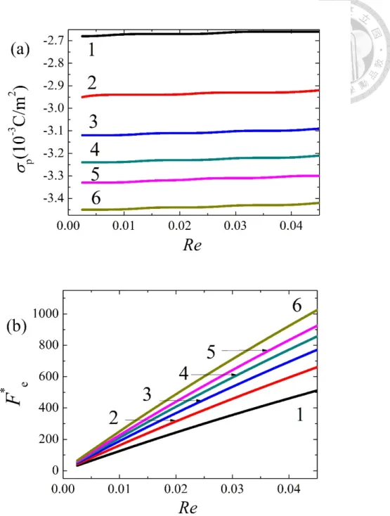
1-3.2 Influence of Reynolds Number

Figure 1-7 demonstrates that how the Reynolds number has an impact on the averaged surface charge density and the scaled electric force. As can be seen in Figure 6(a), the averaged surface charge density has only a slightly increase responding to the increase of Re, this phenomenon will be discussed later. Being different from the averaged surface

doi:10.6342/NTU201801261

11

charge density, the scaled electric force makes an obvious increase with respect to the enlarging Re. The larger F_e^* results from two factors: the large electric potential gradient

and the large space which contains the steep potential gradient. In this case, the increasing Re contributes to the higher amount of the counter ions that is dragged away, causing the

potential gradient getting larger, which results in a larger F_e^* .

Figure 1-8(b) shows the variations of the magnitude of the scaled electric force, F_e^*

with Re for various value of pH, which reveals that the more the pH deviates from the isoelectric point, the greater the F_e^* , which has been discussed in Figure 1-6(b). The behavior of F_e^* corresponds to Re is similar to that of Figure 1-7(b). We choose to

present the variation of the averaged surface charge density for different values of Nt, while we only present the variation of the surface charge density with pH at Re=0.01 here. This is because the value of the averaged surface charge density is almost the same in this range. It should be noticed that when we expand the upper limit to Re=1, the results will be

completely different.

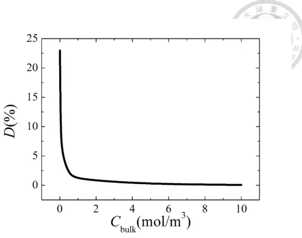
Figure 1-9 shows the variation of the percentage difference in the averaged surface charge density | ^{( 0.0025) ( 1)}| 100%

( 0.0025)

Re Re

D Re

σ σ

Ρ σ Ρ

Ρ

= − =

= ×

= . This figure reveals that the

lower the Cbulk the larger the D. At Cbulk=0.01 mol/m³, D=22.96 %. The variation in the percentage difference in the surface charge density

( 0.0025) ( 1)

| | 100%

( 0.0025)

Re Re

D Re

σ σ

Ρ σ Ρ

Ρ

= − =

= ×

= with pH shown in Figure 1-10. As can be seen,

doi:10.6342/NTU201801261

12

D decreases with increasing pH with the largest D of 11.20 % occurs at pH 5.

1-3.4 Influence of Particle Radius

The results illustrated in Figure 1-11 suggest that the smaller the particle the higher its averaged surface charge density. This can be explained by the difference between the concentration of K⁺ near the particle and the corresponding bulk concentration of K⁺ (CK+- CK+

,bulk) shown in Figure 1-12 for two particle radii. This figure reveals that the distribution of (CK+-CK+

,bulk) for a smaller particle (Rp=75 nm) is more nonuniform than that for a larger particle (Rp=300 nm). In addition the value of (CK+-CK+

,bulk) in Figure 1-13 shows that the value of difference at Rp=75 nm is the largest and that the value of difference at Rp=300 nm is the smallest, implying that the [H⁺] (Rp=75 nm)<[H⁺] (Rp=100 nm)<[H⁺] (Rp=150 nm)<

[H⁺] (Rp=200 nm)< [H⁺] (Rp=300 nm). Therefore, according to Eq. (6), the surface charge density at Rp=75 nm is higher than that at Rp=300 nm, which is seen in Figure 1-11. Figure 13 also demonstrate the value of (CK+-CK+

,bulk) decrease with declining Re, which is attributed to the effect of the drag-away of the couterions. The phenomenon leads to a

decrease in the averaged surface charge density as Re increases. The percentage difference in the averaged surface charge density as Re varies from 0.0025 to 0.04,

( 0.0025) ( 0.04)

' | | 100%

( 0.0025)

Re Re

D Re

σ σ

Ρ σ Ρ

Ρ

= − =

= ×

= , for Rp=75 nm is 8.50 %, and is 0.96 % for Rp=300 nm.

doi:10.6342/NTU201801261

13

The distributions of the surface charge density σΡ along the particle surface from its

south pole (s=0) to its north pole (s=π ) for various values of particle size R^p are presented in Figure 1-14, and those for various values of the Reynolds number Re presented in Figure 1- 15. Figure 1-14 reveals that the smaller the particle the more non-uniform the surface charge distribution. For example, the percentage differences in the surface charge density,

s

( 0) ( )

| | 100%

( 0)

s s

D s

σ σ π

Ρ σ Ρ

Ρ

= − =

= ×

= for Rp=75, 100, 150, 200, and 300 nm are 3.07, 2.33, 1.83, 1.25, and 0.95 %, respectively. This can be explained by the smaller the particle the more significant the degree of double layer polarization. Because the amount of counterions dragged away from the double layer of the particle increases with increasing Re, resulting in a larger Ds, as seen in Figure 1-15.

1-3.5 Influence of Density of Functional Groups

The influences of the density of the functional groups of a particle N_t on its averaged surface charge density σΡ and the magnitude of the scaled electric force acting on it Fe*

are presented in Figure 1-16(a) indicates that the larger the N_t the higher the σ_Ρ, which is expected since the larger the N_t the more the number of functional groups available for dissociation. The trend of Fe* as Re increases seen in Figure 1-16(b) can be explained by that the larger the Re the more the amount of ions is dragged away from the particle.

Figure 1-17(a) reveals that the averaged surface charge density of a particle σΡ increases

doi:10.6342/NTU201801261

14

with increasing bulk salt concentration Cbulk. The rationale behind this is mentioned in the discussion of Figure 6. Note that in Figure 1-17(b) the curve of Fe* at Cbulk=0.1 mol/m³ intersects with that at Cbulk=1 mol/m³. This can be explained by Figure 1-4(b), where the Cbulk

at which the local maximum of Fe* occurs shifts from ≅0.1 mol/m³ to 1≅ mol/m³ as Nt

increases from 5 10 mol/m× ^{−7 2} to 2 10 mol/m× ^{−6 2}.

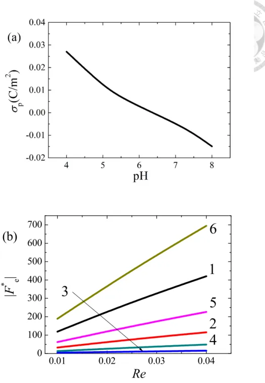
1-3.6 Influence of pH

The behavior of the magnitude of the scaled electric force acting on a particle as pH varies shown in Figure 1-18 is similar to that of the averaged surface charge density seen in Figure 1-8(a). This is expected because the more the pH deviates from the isoelectric point of the particle the higher its charge density and, therefore the greater the electric force acting on it.

As the Reynolds number Re is raised from 0.01 to 0.04, the amount of the counterions dragged away from the particle increases accordingly, resulting in a stronger potential gradient and, therefore, a stronger electric force.

The results illustrated in Figure 1-19 are consistent with those shown in Figure 1-18, that is, the more the pH deviates from the isoelectric point of a particle the greater the electric force acting on it. As observed in Figure 1-6(b), F_e^* shows a local maximum at Cbulk

1 .

≅0 mol/m³.

doi:10.6342/NTU201801261

15

1-4. Conclusions

Taking account of the effect of double layer polarization, the sedimentation of a pH- regulated nanoparticle subject to a generalized gravitation field is modeled theoretically. The radius and the density of the functional groups of the particle, the pH and the bulk salt concentration Cbulk of the liquid phase, and the Reynolds number Re are examined for their influences on the sedimentation behavior of the particle. We show that as the bulk salt concentration varies, the sedimentation velocity of the particle has a local maximum

occurring at Cbulk≅0.1 mol/m³. This arises from the dependence of the concentration of H⁺, and therefore, the charge density of the particle, with Cbulk. As Re increases, more

counterions are dragged away from the particle, yielding a greater electric force acting on it, but its averaged surface charge density becomes smaller.

References

1. O'Melia, C. R., Coagulation and Sedimentation in Lakes, Reservoirs and Water Treatment Plants. Water Sci. Technol. 1998, 37, 129-135.

2. Whitmer, J. K.; Luijten, E., Sedimentation of Aggregating Colloids. J. Chem. Phys. 2011, 134, 034510.

3. Buzzaccaro, S.; Tripodi, A.; Rusconi, R.; Vigolo, D.; Piazza, R., Kinetics of Sedimentation in Colloidal Suspensions. J. Phys.: Cond. Mat. 2008, 20, 494219.

doi:10.6342/NTU201801261

16

4. Song, D.; Jin, H; Jin, J.; Jing, D., Sedimentation of Particles and Aggregates in Colloids Considering both Streaming and Seepage. J. Phys. D: Appl. Phys. 2016, 49, 425303.

5. Yeh, L.H.; Liu, K. L.; Hsu, J. P., Importance of Ionic Polarization Effect on the Electrophoretic Behavior of Polyelectrolyte Nanoparticles in Aqueous Electrolyte Solutions. J. Phys. Chem. C 2011, 116, 367-373.

6. Hsu, J. P.; Tai, Y. H., Effect of Multiple Ionic Species on the Electrophoretic Behavior of a Charge-Regulated Particle. Langmuir 2010, 26, 16857-16864.

7. Chen, Y. Y.; Hsu, J. P.; Tseng, S., Electrophoresis of pH-regulated, Zwitterionic Particles:

Effect of Self-induced Nonuniform Surface Charge. J. Colloid Interface Sci. 2014, 421, 154-159.

8. Bhattacharyya, S.; Gopmandal, P. P., Migration of a Charged Sphere at an Arbitrary Velocity in an Axial Electric Field. Colloids Surfaces A 2011, 390, 86-94.

9. Bhattacharyya, S.; Gopmandal, P. P., Interaction of Electroosmotic Flow on

Isotachophoretic Transport of Ions. Int. J. Math., Comp., Phys., Elec. Comp. Eng. 2012, 6, 1336-1342.

10. Bhattacharyya, S.; Gopmandal, P. P., Effects of Electroosmosis and Counterion

Penetration on Electrophoresis of a Positively Charged Spherical Permeable Particle. Soft Matter 2013, 9, 1871-1884.

11. Gopmandal, P. P.; Bhattacharyya, S., Nonlinear Effects on Electrokinetics of a Highly

doi:10.6342/NTU201801261

17

Charged Porous Shere. Colloid Polym. Sci. 2014, 292, 905.

12. Sonnefeld, J.; Löbbus, M.; Vogelsberger, W., Determination of Electric Double layer Parameters for Spherical Silica Particles under Application of the Triple Layer Model Using Surface Charge Density Data and Results of Electrokinetic Sonic Amplitude Measurements. Colloids Surfaces A 2001, 195, 215-225.

13. Atalay, S.; Barisik, M.; Beskok, A.; Qian, S., Surface Charge of a Nanoparticle Interacting with a Flat Substrate. J. Phys. Chem. C 2014, 118, 10927-10935.

14. Keller, F.; Feist, M.; Nirschl, H.; Dörfler, W., Investigation of the Nonlinear Effects during the Sedimentation Process of a Charged Colloidal Particle by Direct Numerical Simulation. J. Colloid Interface Sci. 2010, 344, 228-236.

15. Keh, H. J.; Ding, J. M., Sedimentation Velocity and Potential in Concentrated Suspensions of Charged Spheres with Arbitrary Double-Layer Thickness. J. Colloid Interface Sci. 2000, 227, 540-552.

16. Yeh, P. H.; Hsu, J. P.; Tseng, S., Influence of Polyelectrolyte Shape on Its Sedimentation Behavior: Effect of Relaxation Electric Field. Soft Matter 2014, 10, 8864-8874.

17. Lee, E.; Tong, T. S.; Chih, M. H.; Hsu, J. P., Sedimentation of Concentrated Spherical Particles with a Charge-Regulated Surface. J. Colloid Interface Sci. 2002, 251, 109-119.

18. Cho, E. C.; Zhong, Q.; Xia, Y., The Effect of Sedimentation and diffusion on cellular uptake of gold nanoparticles. Nature Nanotechnol. 2011, 6, 385-391.

doi:10.6342/NTU201801261

18

19. Cui, J.; Faria, M.; Björnmalm, M.; Ju, Y.; Suma, T.; Gunawan, S. T.; Richardson, J. J.;

Heidari, H.; Bals, S.; Crampin, E. J.; Caruso, F., A Framework to Account for

Sedimentation and Diffusion in Particle–Cell Interactions. Langmuir 2016, 32, 12394- 12402.

20. Björnmalm, M.; Faria, M.; Chen, X.; Cui, J.; Caruso, F.; Dynamic Flow Impacts Cell–

Particle Interactions: Sedimentation and Particle Shape Effects. Langmuir 2016, 32, 10095-11001.

doi:10.6342/NTU201801261

19

Figure 1-1. Sedimentation of a rigid, pH-regulated sphere of radius Rp and surface _Ωp

subject to a generalized gravitational field Cg with g being the gravitational acceleration.

For numerical solution purpose, a large cylindrical computation domain of radius b, length l, and surfaces Ω , _t Ω , and _b Ω is defined, and the cylindrical coordinates (r, θ, z) are _l

chosen with the origin at the particle center.

doi:10.6342/NTU201801261

20

Figure 1-2. Variation of the surface charge density of an isolated, spherical silica particle of

radius 58 nm in an aqueous KCl solution with pH at Cbulk=100 mM, N_t = 2.1 sites/nm², pKA=6.38, and pKB=1.87. Discrete symbols: experimental data of Sonnefeld et al.;¹² curve:

present numerical result.

doi:10.6342/NTU201801261

21

0.000 0.01 0.02 0.03 0.04 5

10 15 20 25 30 35

F

/F

Re (a)

0.00 0.01 0.02 0.03 0.04

0.00 0.05 0.10 0.15 0.20 0.25

F

/F

Re

(b)

Figure 1-3. Variation of the scaled electric force (Fe/Fe,ref) acting on a rigid TiO2 particle of radius 300 nm, zeta potential 76.2 mV, and density

ρ

solution with Cbulk=

1.04 10 ×

force/hydrodynamic force)=(Fe/Fh), (b), with the reference Reynolds number Re. Discrete symbols: numerical result of Keller et al.;¹⁴ curve: present numerical results.

doi:10.6342/NTU201801261

22

Figure 1-4. Variation of the averaged surface charge density σΡ, (a), and the scaled electric

force acting on the particle Fe*, (b), with the bulk salt concentration Cbulk for various values of Nt at Re=0.01 and pH 8. Curve 1: N_t = ×5 10 mol/m^{−7 2}; 2: N_t =7.5 10 mol/m× ^{−7 2}; 3: N_t =10 mol/m^{−6 2}; 4: N_t =1.25 10 mol/m× ^{−6 2}; 5: N_t =1.5 10 mol/m× ^{−6 2}; 6:

6 2

t 2 10 mol/m

N = × ⁻ .

doi:10.6342/NTU201801261

23

Figure 1-5. Contours of the concentration difference (CK+- CK+

,bulk) (mol/m³) on the half plane θ=0 at Cbulk=0.1 mol/m³, Re=0.01, pH 8, N_t =10 mol/m^{−6 2}, and Rp=300 nm.

doi:10.6342/NTU201801261

24

Figure 1-6. Variation of the averaged surface charge density of a particle σΡ, (a), and the magnitude of the scaled electric force acting on it F_e^* , (b), with the bulk salt concentration

Cbulk for various levels of pH at Re=0.01 and N_t =10 mol/m^{−6 2}. Curve 1: pH 5; 2: pH 5.5;

3: pH 6; 4: pH 7; 5: pH 7.5; 6: pH 8.

doi:10.6342/NTU201801261

25

Figure 1-7. Variation of the averaged surface charge density σΡ, (a), and the scaled electric

force acting on the particle Fe*, (b), with the Reynolds number Re for various values of Nt at Cbulk=0.1 mol/m³ and pH 8. Curve 1: N_t = ×5 10 mol/m^{−7 2}; 2: N_t =7.5 10 mol/m× ^{−7 2}; 3: N_t =10 mol/m^{−6 2}; 4: N_t =1.25 10 mol/m× ^{−6 2}; 5: N_t =1.5 10 mol/m× ^{−6 2}; 6:

6 2

t 2 10 mol/m

N = × ⁻ .

doi:10.6342/NTU201801261

26

0.01 0.02 0.03 0.04

0 100 200 300 400 500 600

(b)

|F

|

Re

6

5 4 3

2 1

Figure 1-8. Variation of the averaged surface charge density of a particle σΡ, (a), and the magnitude of the scaled electric force acting on it F_e^* , (b), with the bulk salt concentration

Cbulk for various levels of pH at Cbulk=0.1 mol/m³ and N_t =10 mol/m^{−6 2}. Curve 1: pH 5; 2:

pH 5.5; 3: pH 6; 4: pH 7; 5: pH 7.5; 6: pH 8.

doi:10.6342/NTU201801261

27

Figure 1-9. Variation of the percentage difference in the averaged surface charge density

( 0.0025) ( 1)

| | 100%

( 0.0025)

Re Re

D Re

σ σ

Ρ σ Ρ

Ρ

= − =

= ×

= with the bulk salt concentration Cbulk at

6 2

t 10 mol/m

N = ⁻ , Rp=300 nm and pH 8.

doi:10.6342/NTU201801261

28

Figure 1-10. Variation of the percentage difference in the averaged surface charge density

( 0.0025) ( 1)

| | 100%

( 0.0025)

Re Re

D Re

σ σ

Ρ σ Ρ

Ρ

= − =

= ×

= with pH atN_t =10 mol/m^{−6 2}, Rp=300 nm and Cbulk=0.1 mol/m³.