Information Processing Letters 32 (1989) 61-71 North-Holland
24 July 1989
AN LC BRANCH-AND-BOUND ALGORITHM FOR THE MODULE
ASSIGNMENT PROBLEM
Maw-Sheng CHERN
Department of Industrial Engineering National Tsing Htu Universiry, Hsinchu, Taiwan, Rep. China
G.H. CHEN and Pangfeng LIU
Department of Computer Science and Information Engineering National Taiwan University, Taipei, Taiwan, Rep. China
Communicated by K. Ikeda Received 20 July 1988 Revised 10 March 1989
Distributed processing has been a subject of recent interest due to the availability of computer networks. Over the past few years it has led to the identification of several challenging problems. One of these is the problem of optimally distributing program modules over a distributed processing system. In this paper we present an LC (Leas Cost) branch-and-bound algorithm to fiid an optimal assignment that minimizes the sum of execution costs and communication costs. Experimental results show that, for over half of the randomly generated instances, the saving rates exceed 99%. Moreover, it appears that the saving rates rise as the size of the instances increases. Finally, we also introduce two reduction rules to improve the efficiency of the algorithm for some special cases.
Keywordr: Branch-and-bound algorithms, module assignment problem, distributed processing system
1. Introduction
Distributed processing has been a subject of recent interest due to the availability of computer networks. Over past few years it has led to the identification of several challenging problems. One of these is the module assignment problem. Briefly, the problem can be stated as follows. Given a set of m program modules to be executed on a distributed system of n processors, to which processor should each module be assigned? The problem for more than three processors is known to be NP-hard [4]. The program modules may be viewed as program segments or subroutines, and control is transferred between program modules through subroutine calls. Two costs are considered in the problem: execution cost and communication cost. The execution cost is the cost of executing program modules; the communication cost is the cost of communication among processors. The communication cost is actually caused due to the necessary data transmission among program modules. If a program module is not executable on a particular processor, the corresponding running cost is taken to be infinity.
The module assignment problem has been studied extensively for various models, for example see (3,5-7,9-11,13,14,16], and polynomial-time solutions have been obtained for some restricted cases, such as two processors [1,12,15], tree structure of interconnection pattern of program modules [1,4], and fixed communication cost [2]. In this paper, we consider a general model where the number of processors may be any value, the interconnection pattern of program modules may be any structure, and, more important, various constraints such as storage constraint and load constraint may be included. We then present an LC
Volume 32, Number 2 INFORMATION PROCESSING LETTERS 24 July 1989 (Least Cost) branch-and-bound algorithm to find an optimal assignment that minimizes the sum of execution costs and communication costs. The effectiveness of the algorithm is shown by experimental results. Moreover, we introduce two reduction rules to improve the efficiency of the algorithm for some special cases.
2. The model
The model we consider for the module assignment problem is as follows. (i) There are m program modules M,, Mz,. . . , Mm to be executed.
(ii) There are n processors P,, Pz,. . . , P,, available.
(iii) E(M,, P,) is the cost of executing program module h4, on processor P,.
(iv) T( M,, M,, P,, P,) is the communication cost that is incurred by program modules M, and Mj when they are assigned to processor P, and P, respectively. If Mi and Mj are assigned to the same processor, the communication cost between them is assumed to be 0.
(v) The objective is to minimize the sum of the execution costs and communication costs. (vi) There are the following constraints:
(1)
(2)
(3) (4)
Storage constraint: The available storage provided by a processor is limited. Let SUB( P,) denote the storage limit for processor P, and STOR(M,,) denote the amount of storage occupied by program module M,,. If M,,, Mt2, . . . , M, are all assigned to P,, then STOR( M,,) + STOR( MJ
+ . . . + STOR(MJ must not exceed SUB( P,).
Load constraint: The available computational load provided by a processor has an upper bound. Let LUB( P,) denote the computational load upper bound for processor P, and LOAD( M,,) denote the computational load required by program module M,,. If M,,, M,,, , . . , M,, are all assigned to P,, then LOAD( M,,) + LOAD( MJ + . . . + LOAD( MJ must not exceed LUB( P,).
Some subsets of program modules are restricted to the same processor. Some program modules are restricted to some specific processors.
More constraints can be included in the model if necessary. Based on the model, the problem can be mathematically formulated as follows. Let M denote the set of program modules, P the set of processors, and let + be a mapping from M to P, i.e., 4 : M + P. The problem is to minimize
igrE(M., G(W))+ ZE 2 T(M,, 4, 4(W)* ICI(y)) over all feasible mappings 4.
i-l j-i+1
3. A branch-and-bound algorithm
Since a tree structure is a convenient representation of the execution of the branch-and-bound algorithm, we will describe the branch-and-bound algorithm through the generation of the branch-and- bound tree. Each edge in the branch-and-bound tree represents an assignment of a program module to some processor. The nodes at the lowest (m th) level represent complete solutions and all the other nodes represent partial solutions. A node is infeasible if it does not satisfy the constraints, and an assignment of a program module to some processor is infeasible if it leads to an infeasible node. It is clear that if a node is infeasible, then all of its descendants are infeasible. This suggests that whenever an infeasible node is detected, it may be fathomed, thereby preventing the generation of its subtree. For each node, a pair of values Qj and D,j are estimated for all free (not yet assigned) program modules M, and all processors Pj. vi is the minimum increasing cost that is expected for all the free program modules, given that M, is to be
Volume 32, Number 2 INFORMATION PROCESSING LETTERS 24 July 1989 assigned to P!. Let S denote the set of program modules that are included in the corresponding partial solution. qj is estimated as follows:
+ c min
t
E(My, P,) + C T(M,, M., P,, P+cz,)
MyQS+(M,J M,ES
+T(M,. M,, P,, P,) IKE (1, 2 ,..., n} and M_y+ P, is feasible ) , where P+cx, and P+(,, are the respective processors to which M, and Mz were assigned. q, is set to infinity if M, + Pi is infeasible or M,, ---) P, is infeasible for all processors P,. On the other hand, D,, is the minimum increasing cost that is expected for all the free program modules, given that M, is not to be assigned to P,. 4, is estimated as follows:
D,j=min{&lkE {1,2 ,..., n}, k#j}.
In addition to Q, and D,,, two costs, current cost (CC) and expected cost (EC), are computed for each node. The current cost is the cost of the partial solution (complete solution, if the node is at the lowest level) that is represented by the node. Initially, CC = 0 for the root node. For a nonroot node, if the edge to it from its parent node represents the assignment of M, to P,, the current cost is computed by the following equation:
CC=CC,++f,, p,)+ 1 T(M,, M,, p,, P+(k,),
MkES
where CCP denotes the current cost of the parent node, S denotes the set of program modules that are included in the partial solution represented by the parent node, and P+ck, is the processor to which Mk was assigned. Note that for each feasible node at the lowest level, CC is the cost of the corresponding complete solution. On the other hand, the expected cost is the minimum increasing cost that is expected for all the free program modules. It is computed as follows:
EC = min{ lJj tall free program modules M, and all processors P, } .
Thus, for each node, CC + EC is a lower bound on the costs of the complete solutions that will appear in its subtree.
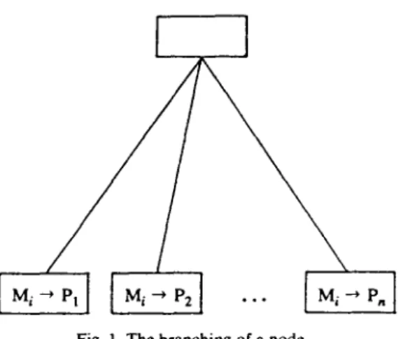
The generation of the branch-and-bound tree starts at the root and follows the LC (Least Cost) strategy [8]. The nodes that wait to be branched are called live nodes. The live node that has a minimum value of CC + CE is selected to be branched next. If a tie exists, break any. When a node is branched, the program module M, that satisfies EC = Uij for some processor P, will be assigned to all processors (see Fig. 1). An upper bound cost (UC) is along with the branch-and-bound algorithm and it represents an upper bound on the optimal cost. UC is set to be infinity intially and is updated to be min{ UC, CC} whenever a feasible node at the lowest level is reached. If a node satisfies CC + EC >, UC, then it is fathomed, since further branching from it will not lead to better solutions. If a node satisfies CC + U,j > UC for some free program module M, and some processor P,, then it is impossible to get better solutions if Mi is to be assigned to Pj. This implies that M, should not be assigned to P, (denoted by M, ++ P,). Thus a node can be fathomed if it satisfies CC + q, 2 UC for some free program module M, and all processors P,. Similarly, if a node satisfies CC + Dij 2 UC for some free program module M, and some processor P,, then M, is restricted to P, (denoted by M, --) P,). These restrictions will cause more nodes to be fathomed.
Volume 32. Number 2 INFORMATION PROCESSING LETTERS 24 July 1989
Fig. 1. The branching of a node.
Finally, when the branch-and-bound algorithm terminates, the value of UC is the optimal cost and the optimal solutions will be generated at the nodes with CC = UC.
The branch-and-bound algorithm is as follows.
Branch-and-hound algorithm
(1)
(2)
(3) (4) (5) (6) (7) (8) (9) (10) (11) (12) (13) (14) (15) (16) (17) (18) (19) (20) (21) (22)set live-node-list to be empty; {live-node-list is a priority queue storing live nodes} put root node into live-node-list and compute IL!,, Dl,, EC. and CC for root node; set UC to be infinity;
while live-node-list is not empty do
begin
choose a node OL with minimum value of CC + EC from live-node-list;
if a has CC + EC > UC or CC + qj > UC for some free M, and all P,, j = 1, 2,. . . , n then remove (2 from live-node-list
else begin
if CC + Qj > UC for some free M, and some P, then a restriction “M, * Pj” is added; if CC + Dij 2 UC for some free M, and some P, then a restriction “M, - Pj” is added;
branch a (assign M, that satisfies EC = y, for some P, to all processors);
for each (assume p) of newly generated nodes do if /I is feasible then begin
compute qj, Di,, EC, and CC;
if /3 is at the lowest level
then if CC < UC then replace UC with CC
else if CC + EC < UC then insert 8 into live-node-list
end;
remove a from live-node-list
end end;
output UC and the nodes (at the lowest level) with CC = UC.
4. Experimental results
In this section we provide experimental results to show the effectiveness of the branch-and-bound algorithm. The criterion we adopt to evaluate the performance of the algorithm is the saving rate, which is 64
Volume 32, Number 2 Table 1
INFORMATION PROCESSING LETTERS 24 July 1989
Saving rates for randomly generated instances
n
-
2 - 3 - 4 - 5 - 6 m 4 i 5 10 - 4" 6" 5r
[O.lOl p-o.2 P-O.5 P-O.8COMMUNCATION COSTS IO.501 0.96047 0.94524 0.94011 0.95107 0.93072 0.91115 0.97087 0.95992 0.94584 0.93919 0.91964 0.94701 0.98114 0.96668 0.92447 0.92701 0.95789 0.97743 0.98539 0.97152 0.96683 0.95228 0.97015 0.98432 0.99313 0.98723 0.98151 0.98244 0.97384 0.98986 0.98985 0.98431 0.96492 0.97630 0.98292 0.99671 0.99552 0.98761 0.96805 0.97910 0.98860 0.99511 0.99419 0.98428 0.98315 0.98531 0.99272 0.99681 0.99732 0.98750 0.97985 0.98997 0.99576 0.99841 0.99773 0.98429 0.98527 0.99602 0.99685 0.99922 0.99713 0.99446 0.99496 0.98682 0.99847 0.99935 0.99862 0.99207 0.98996 0.99391 0.99868 0.99983 0.99888 0.99738 0.99420 0.99533 0.99934 0.99986 0.95109 0.95109 0.94285 0.97767 0.96669 0.96614 0.98615 0.98414 0.97298 0.99489 0.99325 0.99325 0.99830 0.99634 0.99271 0.99867 0.99789 0.99525 0.99956 0.99802 0.99744 0.99970 0.99765 0.99676 0.99955 0.99896 0.99710 0.93461 0.96120 FJ:K ::m 8:E 0.99990 0.94780 0.94780 0.9454’: 0.94310 0.90557 0.93372 0.98344 0.97289 0.97465 0.97992 0.97875 0.97172 0.99454 0.99i76 0.99088 0.98736 0.98443 0.98472 0.99775 0.99574 0.99515 0.99453 0.99003 0.99090 0.99923 0.99789 0.99750 0.99347 0.99165 0.99828 0.99957 0.99904 0.99871 0.99827 0.99671 0.99753 0.99982 0.99957 0.99883 0.99852 0.99736 0.99933 0.89743 0.89743 0.8910: 0.88461 0.87820 0.87820 0.89743 0.89743 0.8974? 0.97055 0.96414 0.9654; 0.96927 0.96670 0.95390 0.96414 0.96158 0.9500E 0.99078 0.99052 0.9882: 0.99180 0.98259 0.97380 0.98899 0.97772 0.9074: 0.99790 0.99703 0.9927t 0.99170 0.98709 0.98540 0.99441 0.99139 0.99267 0.99894 0.99858 0.9981' 0.99751 0.99183 0.99298 0.99543 0.99145 0.99798 0.99981 0.99955 0.9986; 0.99832 0.99833 0.99725 0.99943 0.99675 0.99875 0.99993 0.99971 0.9988! 0.99901 0.99835 0.99924 0.99849 0.99898 0.9997s 0.92664 0.92664 0.92664 0.92200 0.92664 0.92200 0.92200 0.92664 0.92200 0.98083 0.98392 0.97851 0.98315 0.97543 0.96540 0.97852 0.97389 0.96308 0.99629 0.99372 0.9953s 0.99217 0.98883 0.98626 0.99320 0.98844 0.99191 0.99921 0.99820 0.99794 0.99440 0.99460 0.99631 0.99625 0.99610 0.99687 0.99937 0.99864 0.99886 0.99763 0.99801 0.99620 0.99867 0.99860 0.99838 0.99992 0.99961 0.99885 0.99962 0.99788 0.99926 0.99960 0.99811 0.99975
p-o.2 p-o.5 psO.8
IO.1 001 p-o.5 0.92681 0.94819 0.96844 E%tF4 0.99298 0.99705 %E ::E 8:Ei D-O.0 0.95655 0.97204
:::z;‘:
0.99499%:%I
:%I1
EE
0.99992 0.99995 0.91483 0.92802 0.93626 0.94309 0.95846 0.96669 0.98634 0.96969 0.98908 0.98343 0.98252 0.99410 0.98442 0.99100 0.99734 0.99087 0.99728 0.99915 0.99384 0.99787 0.99946 0.99334 0.99900 0.99987 0.99918 0.99950 0.99992 0.94310 0.93137 0.94545 0.97113 0.96058 0.95882 0.99102 0.97462 0.98209 0.99398 0.99043 0.99306 0.99217 0.99622 0.99752 0.99495 0.99564 0.99951 0.99869 0.99912 0.99971defined to be 1 - (N(n - l)/(nm+r - l)), where N is the number of nodes that are actually generated by the branch-and-bound algorithm and
(nmf
’
- l)/(n - 1) is the number of nodes in the complete (unbounded) tree. Since the constraints introduced in the model have a great influence on the saving rate, we do not take them into account in the experiment (it is clear that we would get higher saving rates if the constraints were considered). We make the following assumptions in the experiment:(1) Execution costs are given randomly from [O,lOO].
(2) Communication costs are given randomly from [O,lO], [0,50], and [O,lOO].
(3) Any two program modules have the same probability p to communicate with each other during program execution. p = 0.2, 0.5, 0.8 are considered.
(4) Five instances are run for each case and the average saving rate is computed.
Table 1 shows the resulting saving rates. For over half of the generated instances the saving rates exceed 99%, and it appears that the saving rates will be higher for larger-size instances.
Volume 32, lrlumber 2 INFORMATION PROCESSING LETTERS 24 July 1989
Besides, we also compare optimal costs with those obtained by the random assignment method. The random assignment method randomly assigns each program module to a processor. We assume that execution costs and communication costs are given randomly from [O,lOO] and [OSO] respectively. There is a load constraint on each processor. The LOAD( Mi)‘s are given randomly from (0,501 and each processor has the same value of
LUB= $ * f LOAD( i-l
Table 2
Comparison of optimal costs with costs obtained by random assignment method
m=4 m=5 m=6 m=7 m=8 m=9 m=lO Optimal cost 172 161 115 108 89 183 147 119 173 172 193 202 130 147 45 208 164 149 110 215 260 175 207 150 287 260 272 222 253 106 296 73 220 339 375
Random assignment method Number of Greatest successes cost 38 482 34 574 31 415 21 370 23 425 37 628 37 476 23 722 32 560 38 621 36 678 25 547 20 589 32 646 31 581 35 871 34 803 29 733 24 497 34 813 35 993 22 899 36 985 32 885 31 1255 38 1158 19 1042 28 1105 39 1126 31 1010 35 1255 24 1289 32 1250 31 1478 33 1619 Least Average cost cost 185 370 192 366 131 212 119 258 188 298 196 397 167 330 144 471 217 411 259 440 335 471 255 419 319 452 283 495 282 410 351 618 298 558 290 491 225 389 375 564 531 798 397 544 460 687 370 655 665 937 561 867 629 849 506 749 451 851 388 688 691 951 458 924 642 977 869 1103 927 1266
Volume 32, Number 2 INFORMATION PROCESSING LE-ITERS 24 July 1989 The experiment is performed for n = 4, m = 4, 5,. . . , 10, and p = 0.5. Five instances are randomly generated for each value of m, and 50 random assignments are made for each instance. Among the 50 random assignments, the number of successful (feasible) assignments is computed, and the greatest cost, the least cost, and the average cost are given for the successful assignments. Table 2 shows the experimental results.
5. Two reduction rules
If constraints do not cause interference among program modules (for example, the first three con- straints in the model cause interference among program modules), the following two reduction rules can be implemented for fathoming more nodes. Let C,, denote the maximum communication cost that is incurred by M,, given that M, is to be assigned to Pi. That is,
C,i= 5 max{T(M,. M,, P,, P,)Ir=l,2 ,..., n}. r-l.r+-i
We then have the following property.
Property 1. Zf E(M,, Pk)aE(Mi,P,)+C,j for k=l,2 ,_._, j-l,j+l,._., n, then there exists an optimal assignment in which M, is assigned to P,.
Proof. Suppose that J/* is an optimal assignment in which M, is assigned to P, (u #j). Then we can construct an assignment +’ from $* by changing the assignment of M, from PO to Pi. Let A* be the total cost of $* and A’ be the total cost of $‘. We have
d-A*
=
E(M,, p,) + f
T(M,,
M,, p,,
+‘(M,))
r--l,r#i-E(M,, P,)-- f
T(M,, 4, P,v
4*(
r-1,rti Q E(M,, p,) -Et& P,) -+ r-1,rfi <E(M,, Pj)-E(M,, P”)+C,j<O. So, #’ is an optimal assignment. 0Suppose that M, only communicates with Mu. Let SS,,,, denote the maximum total cost that is incurred by the set {M,, Mu }, given that M, and Mu are to be assigned to the same processor, and SR,, denote the minimum total cost that is incurred by the set {M,, Mu}, given that M, and Mu are to be assigned to different processors. That is,
ss,, =
m={E(M,, P,)+E(M,, P,)lj=1,2 ,..., n},SR mm =fin{E(M,,P,)+E(M,,P,)+T(M,,M,,P,, P,)lj,u~{1,2 ,..., n}and j+o}. We then have the following property.
Volume 32, Number 2 INFORMATION PROCESSING LETTERS 24 July 1989
Property 2. If M, only communicates with MU and SS,,, < SR,,, then there exists an optimal assignment in which both M, and MU are assigned to the same processor.
Proof. Suppose that $* is an optimal assignment in which M, and MU are assigned to P, and P,, j + u,
respectively. Then we can construct an assignment +’ from q* by changing the assignment of M, from P, to P,. Let A* be the total cost of IJJ* and A’ be the total cost of $‘. We have
A’-A* = E(M,, P,) - [E(M,, p,) + T(M,, M,, p,, P”,]
=[E(Mi* Pu)+E(Mu, pu)]-[~(M,, P,)+E(Mu, P,_*)+T(M,. Mu, P,, PO)]
<SS_-SR,,<O So, 4’ is an optimal assignment. 0
6. Concluding remarks
Sinclair [14] has proposed a branch-and-bound algorithm for solving the module assignment problem with the same model except that no constraints are included. In his algorithm a maximal set of independent modules (that do not communicate with one another) is first found and these modules will be assigned after other modules. The lower bound is estimated under the assumption that there is no communication among free modules. Thus it is unnecessary to expand a node if the free modules on the node are independent of one another. Unfortunately, this is not true if constraints are taken into consideration. In this paper, using a different branch-and-bound algorithm, we have solved the module assignment problem with constraints. The experimental results show that the algorithm has an accurate estimation of the lower bound.
Acknowledgment
The authors wish to thank the Editor and anonymous referees for their helpful suggestions and comments.
Appendix: An example
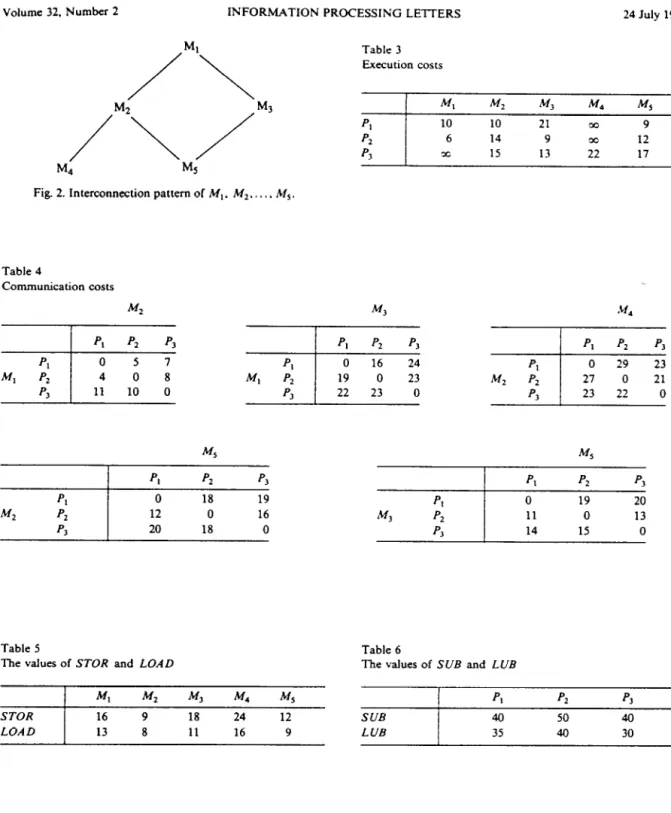
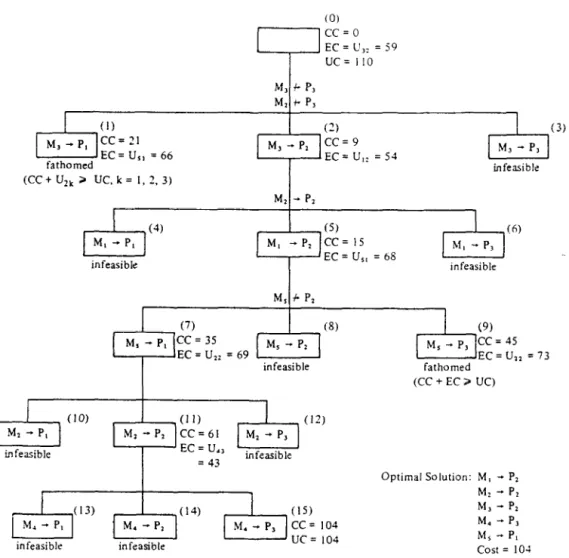
Suppose that there are five program modules M,, M2,. . . , MS and their interconnection pattern is shown in Fig. 2, where Mj-Mj means that M, communicates with M, during execution. There are three processors P,, Pz and P3 available. The execution costs and communication costs are shown in Table 3 and Table 4 respectively. There are storage constraints and load constraints imposed on processors. The values of STOR and LOAD for each program module are shown in Table 5 and the values of SUB and LUB for each processor are shown in Table 6. M, and M, are restricted to the same processor, M, is restricted to P, and P2, and M4 is restricted to P3. To have the illustration simpler, we assume that an initial feasible solution M, --f P,, M, - P,, M3 + Pz, M4 --) P3, M, + P,, whose cost is 110, is obtained by heuristics. The branch-and-bound tree is shown in Fig. 3, where “M, ---) Pj” in each node means “assign program module M, to processor P,“. But, “M, + P,” on an edge represents the restriction that program module M, is restricted to processor P, and “M, + Pj” on an edge represents the restriction that program module M, is not allowed to be assigned to processor P,. The numbers in parentheses represent the
Volume 32, Number 2 INFORMATION PROCESSING LETTERS 24 July 1989
/M’\
/M2\
/M3
M4 M5
Fig. 2. Interconnection pattern of M,. M,. . , M,.
Table 3 Execution costs
Table 4
Communication costs
Table 5
The values of STOR and LOAD
M, Mz M, J% M,
STOR 16 9 18 24 12
LOAD 13 8 11 16 9
Table 6
The values of SUE and LUB PI SUB 40 LUB 35 p2 50 40 PI 40 30
sequence in which the nodes are generated. The values of CC and EC are also shown in Fig. 3. Tracing Fig. 3, we can find that the optimal solution is M, + P2, ii-f, -+ Pz, M3 + Pz, M4 + P3, kf, -B P,, the cost of which is 104.
Volume 32, Number 2 INFORMATION PROCESSING LETTERS 24 July 1989 cc=0 EC = U,: = 59 UC= 110 (I) cc=21 fathomed EC=Ur, =66 (3
cc=
9 EC=U,: =54 infeasible (CC + U,, > UC, k = I, 2, 3) (4) M, - P, infeasible Mz - P, (5) Ml -.P, cc=15 EC = U,, = 68 I (6) hl, _ P, infeasible I (8) infeasibledI
(9) MI . ..p. CC=45 EC = u,, = 73 fathomed __ (CC + EC 2 UC) (10) (12) infeasible infeasible infeasibleFig. 3. The branch-and-bound tree.
References
[l] R.K. Arora and S.P. Rana, On module assignment in two-processor distributed systems, Inform. Process. Lelr. 9 (1979) 113-117.
[2] R.K. Arora and S.P. Rana, Analysis of the module assign- ment problem in distributed computing systems with limited storage. Inform. Process. L&t. 10 (1980) 111-115. [3] S.H. Bokhari, Dual processor scheduling with dynamic reassignment, IEEE Trans. Soft-ware Eng. SE-5 (1979)
341-349.
[4] S.H. Bokhari, A shortest tree algorithm for optimal as- signments across space and time in a distributed processor system, IEEE Truns. So/fware Eng. SE-7 (1981) 583-589. [5J T.L. Casavant and J.G. Kuhl, A taxonomy of scheduling in general-purpose distributed computing systems. IEEE
Trans. Soffware Eng. SE-14 (1988) 141-154.
Optimal Solution: M, - P2 MI - P, M, - P* M, - Pa M, - P, cost = 10-l
[6] W.W. Chu and L.M.-T. Lan, Task allocation and prece- dence relations for distributed real-time systems, IEEE Tram. Compur. C-36 (1987) 667-679.
[7] C. Gao, J.W.S. Liu and M. Railey, Load balancing al- gorithms in homogeneous distributed systems, In: Proc. 1984 Internor. Conf on Parallel Processing (1984) 302-306.
18) E. Horowitz and S. Sahni, Fundamentak of Compuler Algorirhms (Computer Science Press, Potomac, MD, 1978). (91 B. Indurkhya, H.S. Stone and X.-C. Lu, Optimal parti-
tioning of randomly generated distributed programs, IEEE Trans. Sofware Eng. SE12 (1986) 483-495.
[lo] V.M. Lo, Heuristic algorithms for task assignment in distributed systems, IEEE Trans. Compur. C-37 (1988) 1384-1397.
Volume 32, Number 2 INFORMATION PROCESSING LEITERS 24 July 1989 model for distributed computing systems, IEEE Trans.
Compur. C-31 (1982) 41-47.
[12] G.S. Rao, H.S. Stone and T.C. Hu, Assignment of tasks in a distributed processor system with limited memory, IEEE Trans. Cornput. C-28 (1979) 291-299.
[13] C.C. Shen and W.H. Tsai, A graph matching approach to optimal task assignment in distributed computing systems using a minimax criterion, IEEE Trans. Cornput. C-34 (1985) 197-203.
[14] J.B. Sinclair, Efficient computation of optimal assign- ments for distributed tasks. J. Parallel Disrribuled Com-
put. 4 (1987) 342-362.
[IS] H.S. Stone. Multiprocessor scheduling with the aid of network flow algorithms, IEEE Trans. Software Eng. SE-3 (1977) 85-93.
1161 H.S. Stone and S.H. Bokhari, Control of distributed processes. Computer I1 (1978) 97-106.