CHAPTER 4 DESIGN AND IMPLEMENTATION

CHAPTER 4 DESIGN AND IMPLEMENTATION

In this chapter, we describe how to rebuild an interactive 3D environment with non-blocking scene streaming feature. First of all, an overlapped file I/O subsystem is implemented and receives I/O request packets to do file operation, which is running in the background. Next, we make use of ray-casting technique to modify the original section files and calculate the distance between each section. Furthermore, with this information above, we estimate the adequate distance to add directives in the original section files for loading of possibly oncoming sections. Finally, we design a cache management mechanism for pre-reading and simulate cache operation to retain our data in memory for future loading.

4.1 Overlapped File I/O

There are four methods of implementing our overlapped file I/O subsystem under windows operating system, which are Signaled File Handles, Signaled Event Objects, Asynchronous Procedure Calls(APCs), and I/O Completion Port separately. For Signaled File Handles, it uses file handles and an OVERLAPPED structure which contains essential I/O request parameters to invoke ReadFile function, and the operating system will process our request in the background. For Signaled Event Objects, it exploits an event object for an overlapped I/O request, and the event object

is set to the signaled state when the overlapped I/O operation has been completed. In addition, a single thread can specify different event objects in several simultaneous overlapped operations. For APCs, it uses a callback function which is also termed I/O completion routine. The I/O completion routine gets called when the thread is in an alertable state and an overlapped I/O operation has completed. The three mechanisms mentioned above, however, have some natural drawbacks; therefore we take advantage of I/O completion port in our approach.

I/O completion port is the mechanism by which an application uses a pool of threads that was created when the application was started to deal with overlapped I/O requests. These threads are created for the sole purpose of processing I/O requests.

Applications that cope with many concurrent overlapped I/O requests can do so more quickly and efficiently by using I/O completion ports than by using creating threads at the time of the I/O request.

When a file is opened by overlapped I/O, we can associate its file handle with an I/O completion port. Once we have set up this association, the I/O system sends an I/O completion notification packet to the I/O completion port when the I/O operation completes. This action is performed within the operating system and transparent to applications. In response to I/O completion packet, completion port releases a waiting thread to process it. This thread is still one of the original waiting threads assigned to

the I/O completion port, except that it is active. As soon as the active thread finishes processing the I/O request, it will become waiting again of the I/O completion port.

Based on such mechanism, we implement an overlapped file I/O subsystem which receives I/O requests from memory management system. We may consider the subject under four steps: (1) create an I/O completion port and associate it with a file handle; (2) create a number of threads; (3) let each thread be waiting on the completion port; (4) issue some overlapped I/O requests to operate that file. We shall describe them in detail as follows.

To begin with, we invoke the CreateIoCompletionPort function to create an I/O completion port. This function associates an I/O completion port with one or more file handles. The first parameter is a file handle and we have to specify the

FILE_FLAG_OVERLAPPED flag when using the CreateFile function to obtain the

handle. For the most part, CreateIoCompletionPort() is called twice. For the first time, we set parameter FileHandle as INVALID_HANDLE_VALUE and

ExistingCompletionPort as NULL, so as to create a port without any association with

file handles. Successively CreateCompletionPort() is invoked for any file handle which would be associated with a completion port. We must specify the parameter

ExistingCompletionPort as the handle obtained from the first calling of

CreateIoCompletionPort(). Figure 4.1 indicates some sample code about what we

have mentioned. In addition to these, the I/O system can be instructed to send I/O completion notification packets to I/O completion ports where they are queued.

Figure 4.1 Sample code

Next, we can create some worker threads waiting on the completion port. We may note that the I/O completion port doesn’t create any waiting thread spontaneously;

it just uses threads created by ourselves. Once these threads are created, they will be waiting for future I/O requests. It is worth pointing out, in passing, that these threads can do nothing but tasks involve in a completion port since they are addicted to the completion port.

While some threads are dealing with I/O requests, the statuses of all threads in the pool are as follows,

executing threads + blocking threads + waiting threads on the completion HANDLE hPort;

HANDLE hFiles[MAX_FILES];

int index;

//Create the completion port

hPort = CreateIoCompletionPort (INVALID_HANDLE_VALUE, NULL, 0, 0);

//Now associate each file handle

for (index = 0; index < OPEN_FILES, ++index) { CreateIoCompletionPort(hFiles[index], hPort, 0, 0);

}

= a total of all worker threads in the pool

Therefore, we create threads twice as many as number of CPU. The main reason is that if we have a CPU and create only a thread, our CPU will be idle while the only one thread is blocking for some cause. The completion port cannot provide any service for another I/O request due to the lack of threads in the pool, even if our CPU is available. Since threads are not free, there is no need to create threads without any limitation.

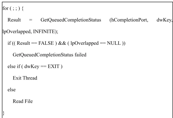
Furthermore, each worker thread calls GetQueuedCompletionStatus function to wait for a completion packet to be queued to that completion port. Threads that wait for execution on a completion port are released in last-in-first-out(LIFO) order to supply services. Since all threads work the same as each other, there is no worry about their working sequence. On the other hand, the GetQueuedCompletionStatus function attempts to dequeue an I/O completion packet from the specified completion port. By calling this function, a running thread can obtain a successive request and keep on executing without blocking. It is likely that a thread would be paged out if it is waiting for a long time. In contrast, a running thread is still residing in system memory and immediately picking up a queued completion packet without context switches, which is more efficient. Figure 4.2 shows a sample pseudo code.

Figure 4.2 a sample pseudo code

Finally, we can use the PostQueuedCompletionStatus function to issue an I/O completion packet to the completion port without starting an overlapped I/O operation.

This is useful for informing worker threads of external notifications. Therefore, main thread or any other thread is able to issue a read operation for a file associated with the completion port.

4.2 A pre-fetch scheme

For our purpose of pre-fetching, we should travel each section in the 3D environment and add directives for pre-loading in the original section. Therefore, we read all section files to load the entire 3D scene firstly. This is done by the TV3D engine, and then we cast a number of rays to detect which meshes and sections we can

for ( ; ; ) {

Result = GetQueuedCompletionStatus (hCompletionPort, dwKey, lpOverlapped, INFINITE);

if (( Result == FALSE ) && ( lpOverlapped == NULL )) GetQueuedCompletionStatus failed

else if ( dwKey == EXIT ) Exit Thread

else

Read File }

see in the current section. The results are saved and used for prompting that some specified sections should be loaded from now on. On the other hand, we exploit a cache management to reserve data in cache for nearly use. All implementation details are described in the following paragraphs.

4.2.1 Recovering a 3D virtual environment

In our approach, we make an assumption that a 3D virtual scene has been partitioned into several sections which are dealt as fundamental streaming units.

These section files were fed to a 3D engine, TV3D; accordingly, a completed 3D scene could be recovered. TV3D, as we have mentioned before, is a complete programming suite accelerating the development of 3D games and applications. We can get rid of implementation details by TV3D and concentrate on our approach.

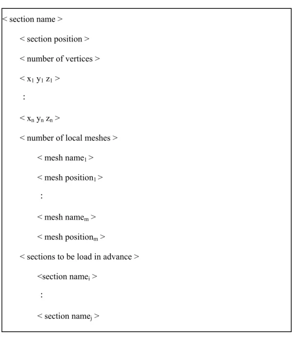
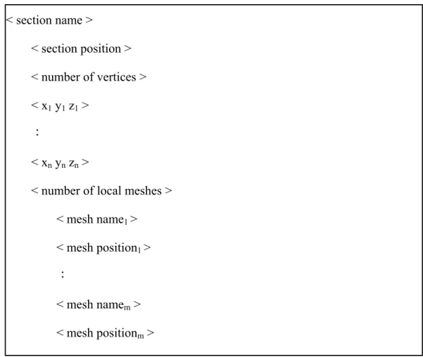
Figure 4.3 illustrates the format of section files, and we explain each tag as follows: <section name> represents this section’s name; <section position> is this section’s position in 3D coordinate; since a section may have three, four, or more edges, we save each coordinate of these vertices in <x₁ y₁ z₁>, …, <x_n, y_n, z_n>

counterclockwise or clockwise and the amount of vertices in <number of vertices>; in addition, there may be some meshes on this section, therefore we record the amount of meshes in <number of local meshes> and their filenames in <mesh name> and coordinates in <mesh position> respectively.

Figure 4.3 Format of section files

After locating this section, we are to process <number of vertices> and their coordinates. For each vertex(i), we use vertex(i) and vertex(i + 1) as two parameters to construct a plane mesh. Consequently, this section is surrounded by n planes. Figure 4.4 indicates an example of what we said. Suppose a mesh ABCD is a simplified section. We use (A, B), (B, C), (C, D), and (D, A) in turn to create four planes, which are ABFE, BCGF, CDHG, and DAEH. The purpose of these vertices is to construct auxiliary meshes which help us to ensure that any required mesh is loaded in advance.

We will describe their functionality in later paragraphs.

< section name >

< section position >

< number of vertices >

< x1 y1 z1 >

：

< xn yn zn >

< number of local meshes >

< mesh name1 >

< mesh position1 >

：

< mesh namem >

< mesh positionm >

Figure 4.4 a simplified section ABCD and four auxiliary planes

While loading these local mesh files, we keep track of their relation. In other words, we take advantage of a map data structure to record mesh filenames and their

IDs within the scene graph. On the other hand, which mesh belongs to this section is

also marked down in a specified table, MeshOfSect. Therefore, we can find out what meshes a section contains quickly and vice versa. In addition to these, we also calculate loading time of each mesh, add them all together and record it in a table,

SectionLoadTime. Finally, we make use of a set data structure to save the loaded mesh

filenames, which is helpful to determine whether one mesh has been loaded.

4.2.2 Casting rays from each section

Now that we are sure that a complete 3D complex scene has been recovered, the next step is to detect which meshes we may see from one section. For this purpose, we cast several rays to surroundings. Figure 4.5 illustrates a simple example: there are four rays casting from section_1, two of them hit mesh_1 and mesh_2 respectively

A B

C E

H G

F D

which are located on another sections, one hits mesh_3 located on section_1, and the other ray hits nothing.

Figure 4.5 a simple example of ray-casting

In our approach, we cast twelve rays horizontally which have interval of thirty degree from one ray to the next. Once a ray hits a mesh, it stops passing through this mesh and returns the distance between start point and impact point. In addition to the returned distance, we are also aware of this mesh which a ray hits. Next, we make use of a tabular search to find out which section this mesh belongs to. With this information, we can create a conservative possibly visible set for each section. The advantage of conservative visibility preprocessing is to prune most of invisible meshes by relatively low cost computation instead of computing exact visibility. To put this more concretely, we use a specified table, SectInSight, and linked-list to

section_1 mesh_2

mesh_1

mesh_3

record every section name which is in sight from local sections. Besides, the loading time of each section is recorded in each node respectively.

To take a simple example, if there are three rays casting from section_1 and hit

mesh_2 located on section_5, hit mesh_3 located on section_9, and hit mesh_4 located on section_4, the SectInSigh table would look like Figure 4.6.

Figure 4.6 a simple example of SectInSight[]

However, there is an exception to the rule. Our rays, for instance, may pass through one section where all local meshes are lower than these rays, and ignore this section, but indeed we can see that section. One solution is to cast more rays in more different angles, but leading to significant system overhead, even this ray-casting is computed off-line. In our approach, we take advantage of auxiliary plane meshes to solve this predicament. These auxiliary will not be loaded during runtime. As we have mentioned earlier, many auxiliary planes were created and surrounding each section.

section_1

section_2

section_5 section_9 section_4 SectInSight[]

LoadTime_5 LoadTime_9 LoadTime_4

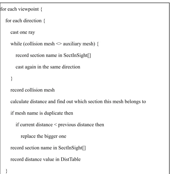
Therefore, our rays will not pass through one section without hitting any mesh. In other words, when a ray enters and leaves a section, it hits two meshes at least so that this section filename is added to SectInSight’s node. After hitting an auxiliary plane, our ray will not stop proceeding in the identical direction until collides with an original mesh. Figure 4.7 is the pseudo code of above conservative possibly visible set method.

Figure 4.7 Pseudo code for each viewpoint {

for each direction { cast one ray

while (collision mesh <> auxiliary mesh) { record section name in SectInSight[]

cast again in the same direction }

record collision mesh

calculate distance and find out which section this mesh belongs to if mesh name is duplicate then

if current distance < previous distance then replace the bigger one

record section name in SectInSight[]

record distance value in DistTable }

4.2.3 Pre-loading with given distance

In order to achieve our purpose of streaming, sections should be loaded during a specified interval before players see those sections. We cast rays from each section and detect which sections are in sight in the previous paragraph. By figure 4.7, we also record their distance in a two-dimensional table, DistTable, which includes the distance from one section to another.

The DistTable is not absolute correct, however, because it only records the range from current section to another sections which can be seen on the current section, exclusive of other sections which are out of sight. To resolve this situation, we use

Floyd’s algorithm which is also know as the all pairs shortest path algorithm. It will

compute the shortest path between all possible pairs of sections in Ο(n³) time where n is the total number of sections.

After computing the shortest path, our DistTable is more accurate and helpful for pre-loading. Since players have basic velocity in gameplay, we compute (velocity of a

player * loading time of sections) to get distance and take it into account when we

need to load section files in advance. For instance, if a player standing on a section,

section_m, can see n sections: section_1, section_2…section_n, we should load the n section files early before he arrives. Accordingly, we begin to load these section files at some sections which are (velocity of a player * loading time of the n sections) away

from the destination. In this way, when a player arrives at section_m, he will see all the n sections without waiting for loading.

Figure 4.8 Pseudo code

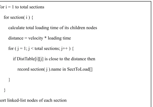
Figure 4.8 illustrates an algorithm to accomplish our goal. First of all, for each

SectInSight[i], we compute the total loading time of its children nodes and obtain the

distance by (velocity of a player * total loading time). Next, we search DistTable to find out those sections which are nearly as far as the distance. Furthermore, these section names are recorded in a data structure which similar to Figure 4.6. We use a specified table, SectToLoad, and linked-list to record every section name which will be loaded in advance. Besides, the loading time of each section is appended to each node respectively. After processing each section and their linked-list nodes, we sort

for i = 1 to total sections for section( i ) {

calculate total loading time of its children nodes distance = velocity * loading time

for ( j = 1; j < total sections; j++ ) {

if DistTable[i][j] is close to the distance then record section( j ).name in SectToLoad[]

} }

sort linked-list nodes of each section

these nodes in an increasing order and write back to original section files. Figure 4.9 shows the format of modified section files. Accordingly, the nearer the section is, the earlier it is loaded.

Figure 4.9 Format of modified section files

In our approach, we consider to use another thread to load sections in the background. Since we construct our system with the TV3D engine, the

< section name >

< section position >

< number of vertices >

< x1 y1 z1 >

：

< xn yn zn >

< number of local meshes >

< mesh name1 >

< mesh position1 >

：

< mesh namem >

< mesh positionm >

< sections to be load in advance >

<section namei >

：

< section namej >

implementation is much engine dependence. The TV3D engine manages memory allocation, scene graph, and rendering without allowing us to exploit another thread to access its inner data structure concurrently. Accordingly, we can only load section files in the main loop with procedures sequentially

On the other hand, because of inability to load files concurrently, we invoke the overlapped file I/O subsystem and cache management to read files and keep them in cache before they are loaded actually in the near future. Therefore, when we need these section files, we are able to load them quickly without serious impact on rendering frame rate.

4.3 A cache management

Now that we are sure that we have modified all of our original section files, the next step is using these files to construct a non-blocking scene streaming 3D virtual environment. Initially, we load part of total section files, inclusive of meshes on local section. On the other hand, we record those section names which are tagged as

<sections to be load in advance> and not to load them right away. Instead of loading

them immediately, we should invoke our overlapped file I/O subsystem to read these section files and then store them in cache for future loading. Accordingly, when a player’s character arrives at some section, the main loop should start to load the sections tagged as <sections to be load in advance> in the current section file.

Because they are cached in advance, they can be loaded as fast as possible.

Since the operating system prohibits us from controlling cache directly, we cannot store data or adjust the resident interval in cache by ourselves. In our implementation, we adopt a compromised mechanism to simulate cache operation.

First of all, when loading sections in the initial stage, we keep track of those sections tagged as <sections to be load in advance>. Secondly, we find out those meshes which are located on these tagged sections and take advantage of a table, MeshToLoad, to store their names. Finally, we create a thread to read these mesh files by names recorded in MeshToLoad infinitely.

To put it clearly, when we record these mesh filenames which are likely oncoming, we issue I/O request packets to our overlapped file I/O subsystem and keep a specified thread reading them continuously. Because our overlapped file I/O subsystem read complete file contents, the specified thread merely reads a block of each section file and the operating system will store the full file contents in cache automatically. Consequently, we don’t worry about those mesh files which are pre-read will be flushed out of memory. On the other hand, some entries of

MeshToLoad will be removed after they are loaded into the 3D scene, and prevent

MeshToLoad from increasing.

This mechanism enables us to benefit from cache without controlling it directly

and when we are loading these meshes which are pre-read, it will cost fewer time without waiting for I/O operation in our hard drive.