國立臺灣大學電機資訊學院電機工程學系 碩士論文
Graduate Institute of Electrical Engineering
College of Electrical Engineering and Computer Science National Taiwan University
Master Thesis
利用強健的全域與區域之無解空間 辨識技術來提升限制性隨機樣本產生效能
Improving Constrained Random Pattern Generation by Powerful Global and Local Infeasible Solution Space Identification
林恩祥 En-Hsiang Lin
指導教授:黃鐘揚 博士
Advisor: Chung-Yang (Ric) Huang, Ph.D.
中華民國 104 年 7 月
July, 2015
i
誌謝
碩士生涯是一個讓我學習成長的過程,感謝指導老師黃鐘揚教授這一路來對 我的指導。特別是他在這一路過程中所對我付出的耐心與包容。
另外特別感謝 Gary 對於論文方向的討論與建議。以及 Rocky、穎哥、阿泡、
紹倫學長、Jason 學長等實驗室成員在這一路上曾經給過的建議與指教。
感謝我周圍的朋友,謝謝 Kphenix 給過的一些建議。
感謝老天給我這個機緣加入 353 實驗室,讓我有更多學習成長的機會。最後感 謝我親愛的家人一直以來無怨無悔的付出與關愛。
林恩祥 2015
ii
中文摘要
功能性驗證在晶片設計流程上是不可或缺的一環。其中,直接測試是工業上最 被廣泛使用的方法。它能在驗證初期快速檢驗電路基本功能。然而,其所產生的測 試向量容易受限於使用者對待測系統的認知而產生分布不均的現象,使得一些角 落錯誤不易觸發,進而影響到待測電路的測試覆蓋率。另一類被稱為限制式随機驗 證的方法在近年來受到了重視。使用者只需根據待測電路規格與驗證的目標撰寫 輸入限制式。接著,限制式求解器會自動產生大量滿足輸入限制式的測試向量。與 直接測試的方法相比,它能快速並有效的產生更多的測試向量來模擬待測電路。
限制式求解技術是整個隨機驗證方法的核心。一個好的限制式求解器應該包 含以下性質:1) 高生產率 2) 均勻分布(機率上) 3) 均勻分布(空間上)。換言之,
它應該要能有效率的快速產生測試向量,並且同時保證產生的測試向量在機率和 解空間角度上是均勻分散的。本篇論文針對一些較為困難的例子去提高測試向量 的產生速率。我們的改進主是要建立在辨識更多的無解空間。當無解空間能辨識愈 多,限制式求解器效率也會進一步提高。
我們把辨識流程分為兩階段:1) 全域無解空間辨識 2) 區域無解空間辨識。
兩者適用在不同的情況。在全域無解空間辨識的階段中,它過濾了包含有可全域式 縮減變數的無解空間。一個變數如果初始範圍可以在不考慮其他變數的賦值下進 行縮減,該變數稱為可全域式縮減變數。我們提出了一個迭代事件驅動的方法搭配 正規詞級解法器去辨識出該類型變數。在區域無解空間辨識的階段,剩下的無解空 間大部份是由可條件式縮減的變數所組成。一個變數如果需在同時考慮部份其他 變數的數值情況下才能進行縮減,稱為可條件式縮減變數。我們使用了既有文獻裡
iii
所提出的範圍切割樹方法來過濾該類型的無解空間。範圍切割樹的樣式顯著地影 響了無解空間辨識的能力。我們建置範圍切割樹的方法是去動態地選擇當下最困 難的一條限制式做切割。實驗結果顯示,這種以貪心為基礎的建置方法能更有效地 辨識出無解空間因此測試向量的生產率能因此大幅提高。
關鍵字:功能性測試、限制式隨機驗證、範圍切割樹
iv
ABSTRACT
Functional verification is indispensable in circuit design flow. Directed testing is the most prevalently used method in industry. It can quickly validate basic functionality of
design under verification (DUV) at the early stage. However, the generated test vectors
are easily biased due to the designers’ perception on the DUV, which lowers the chance to trigger corner bugs. This greatly affects the test coverage of DUV. Another approach called Constraint Random Verification (CRV) draws more attention in recent years. Users provide input constraints based on system specification and their intention for verification, and then a constraint solver would efficiently generate vast amounts of patterns that satisfy the constraints. Compared to former approach, it can quickly generate more effective patterns to simulate the DUV.Constraint solving technique is the key of CRV methodology. A good constraint solver for CRV should have the following properties: 1) high throughput 2) uniform distribution (in probability) 3) high pattern diversity (in search space). In other words, it should efficiently generate valid patterns while ensuring evenness and pattern diversity at the same time. In this thesis, we focus on improving throughput for some rather difficult cases. Our improvements mainly come from the identification of infeasible solution space for the input constraints. Intuitively, as more infeasible solution space is identified, the higher throughput the constraint solver can be achieved.
We divide the identification into two stages: 1) global infeasible space identification 2) local infeasible space identification. They apply to different situations. At global infeasible space identification stage, it filters out infeasible space which consists of universally reducible variables. A variable is universally reducible if its initial range can
v
be reduced without consideration of the assignments of other variables. We proposed an iterative event-driven approach combined with the word-level SMT solver to identify such space. At local infeasible space identification stage, remaining infeasible space is mostly composed of conditionally reducible variables. A variable is conditionally reducible if its range can only be reduced with regard to the assignments of some of other variables. We utilize the Range Splitting Tree (RST) technique to filter out such infeasible space. The structure of constructed RST greatly affects the ability of infeasible space identification. Our RST construction is guided by dynamically selecting the constraint with lowest hit rate on-the-fly. Experimental results show the effectiveness of this greedy based construction to identify infeasible space, and thus the throughput can be substantially enhanced.
Keywords: Functional Verification, Constrained Random Verification, Range Splitting Tree
vi
CONTENTS
口試委員會審定書 ... #
誌謝 ... i
中文摘要 ... ii
ABSTRACT ... iv
CONTENTS ... vi
LIST OF FIGURES ... ix
LIST OF TABLES ... xi
Chapter 1 Introduction ... 1
1.1 Problem Formulation and Supported Constraint Types ... 3
1.1.1 CRV Problem Formulation ... 3
1.1.2 Supported Constraint Types ... 3
1.1.3 Difference between Constraint Satisfaction and Constraint Verification Problem. ... 3
1.2 Related Work ... 4
1.3 Contribution ... 8
Chapter 2 Review of RSSDE technique ... 9
2.1 Flow of RSSDE ... 9
2.2 Preprocessing Stage (RST Construction) ... 11
2.2.1 Properties of Range Splitting Tree (RST) ... 11
2.2.2 Solution Density Estimation by Statistical Approach ... 12
2.2.3 RST Construction Heuristics ... 12
vii
2.3 RST Guided Pattern Generation Stage ... 15
2.4 RSSDE Algorithm ... 16
Chapter 3 Global and Local Infeasible Space Identification ... 19
3.1 Applicability of Global and Local Infeasible Space Identification ... 21
3.2 Global Infeasible Space Identification... 27
3.2.1 Brute-Force Approach ... 28
3.2.2 Depth-Limited Bisection Approach (Single SMT instance) ... 28
3.2.3 Iterative Event-Driven Approach (Multiple STM instances) ... 31
3.3 Local Infeasible Space Identification ... 36
3.3.1 Split by Constant Values ... 38
3.3.2 Split by Infeasible Intervals Detection ... 39
3.3.3 Split by Joint Distribution Analysis of Two Variables ... 42
3.3.4 Split by Random Bisection ... 45
Chapter 4 Discussions and Heuristics ... 46
4.1 Direct Branching Probabilities Estimation by Using Only Leaf Nodes ... 46
4.2 Adaptive Cutting Plane Decision by Biased Distribution ... 47
4.3 Parallel RSTs ... 48
4.3.1 Independent Variables Case ... 48
4.3.2 Dependent Variables Case ... 49
4.4 Direct Constraint-based Infeasible Space Inference ... 50
Chapter 5 Experimental Results ... 51
5.1 Description of Testcases ... 51
5.2 Evaluation of Efficiency and Effectiveness of Infeasible Space Identification ... 53
viii
5.2.1 Comparison of our approach and RSSDE ... 53
5.2.2 Comparison of Depth-Limited and Iterative Event-Driven Approaches at Global Identification Stage ... 56
5.2.3 Comparison of Different SMT Construction Methods at Local Identification Stage ... 59
5.3 Evaluation of Throughput, Evenness and Pattern Diversity ... 62
Chapter 6 Conclusion ... 65
REFERENCES ... 66
ix
LIST OF FIGURES
Fig. 1-1 A typical CRV flow ... 1
Fig. 1-2 An illustration of basic interval propagation flow for x + y < 10. ... 7
Fig. 2-1 The flow of RSSDE ... 9
Fig. 2-2 Two possible RST structures for the same instance ... 13
Fig. 2-3 An example of top-down random walking in RST ... 16
Fig. 2-4 (a) Shows the entire solution space of x + y < 6 or x > y + 6 with 0 ≤ x, y ≤ 10 (b) Shows one possible RST structure. (Modified from [12]) ... 16
Fig. 2-5 The RSSDE algorithm [4] ... 18
Fig. 3-1 Proposed approach versus original approach ... 21
Fig. 3-2 A possible RST structure for Example 3-1 ... 22
Fig. 3-3 An extended RST structure from Fig. 3-2. ... 23
Fig. 3-4 A smaller RST structure by applying global infeasible space identification first. ... 24
Fig. 3-5 Naïve interval propagation does not further reduce range of x2. ... 25
Fig. 3-6 An illustration of feasible but not sampled points ... 28
Fig. 3-7 The depth-limited bisection approach ... 30
Fig. 3-8 An example of multiple SMT instances ... 33
Fig. 3-9 The iterative event-driven approach ... 34
Fig. 3-10 Branch variable & cutting plane decision procedure ... 37
Fig. 3-11 An illustration of different SMT construction methods for TARGET ... 40
Fig. 3-12 Split by infeasible intervals detection procedure ... 41 Fig. 3-13 Two infeasible space occupy different proportions of search space. (This
x
figure is not drawn to scale)... 43
Fig. 3-14 An illustration of 8-by-8 0-1 matrix ... 44
Fig. 3-15 Split by joint distribution analysis procedure ... 45
Fig. 4-1 Direct branching probabilities estimation by using only leaf nodes... 46
Fig. 4-2 The green-line partition leads no throughput enhancement. ... 47
Fig. 4-3 An example of 2 RSTs for dependent variables ... 49
Fig. 5-1 Comparison of processing time between ours and RSSDE ... 55
Fig. 5-2 Comparison of pattern throughput between ours and RSSDE ... 55
Fig. 5-3 Comparison of preprocessing time between depth-limited and iterative event driven methods... 58
Fig. 5-4 Comparison of remaining feasible space volume after RST construction between depth-limited and iterative event driven methods ... 58
Fig. 5-5 Comparison of RST construction time for φ1, φ2 and φ3 approaches ... 61
Fig. 5-6 Comparison of feasible volume after RST construction for φ1 and φ3 ... 61
Fig. 5-7 Comparison of overall runtime between ours and VCS® ... 64
Fig. 5-8 Comparison of pattern diversity between ours and VCS® ... 64
xi
LIST OF TABLES
Table 1-1 Supported operators in our work ... 3 Table 1-2 Consecutive 5 patterns produced by boolector shows high correlation problem for direct SAT/SMT-like technique ... 6 Table 3-1 Automatic cutting plane decision depends on constraint format for constant values ... 39 Table 3-2 Different SMT construction methods for TARGET constraint during RST construction... 39 Table 5-1 Statistics of testcases... 52 Table 5-2 Runtime & effectiveness of infeasible space identification between our approach and RSSDE ... 53 Table 5-3 Comparison between depth limited & iterative event-driven approaches .... 57 Table 5-4 Evaluation of different SMT construction methods in building RST ... 60 Table 5-5 The result of throughput & pattern diversity evaluation ... 63
1
Chapter 1 Introduction
Functional verification is always a challenging task for verification engineers. One popular approach is Directed Testing. It requires users to manually provide test vectors and uses them to simulate the system. However, resulted patterns are highly biased. It is because users can barely write test vectors that are beyond their expectations.
Constraint Random Verification (CRV) methodology is aimed to alleviate this
problem. Fig. 1-1 shows the typical CRV flow. It consists of four stages. At first stage, designers specify input constraints to conform to the system specifications. These input constraints are then solved by a constraint solver. Produced test vectors are valid patterns that satisfy all input constraints. Designers use these vectors to simulate the Design underVerification (DUV). Finally, monitors are used to verify and evaluate the response of DUV.
Fig. 1-1 A typical CRV flow
The challenge for CRV constraint solver is how to efficiently and effectively produce vast amounts of patterns to validate system. In the lack of prior knowledge of the search space, generated patterns are suggested to be uniformly distributed in SystemVerilog LRM [1]. Uniform distribution means all feasible patterns are equally probable. However, in some situations, only equal probability may not be sufficient. In [2][3], they suggested solution space should also be evenly explored. In other words, produced patterns should not be clustered in certain local space. In this thesis, we call this target “pattern diversity”
2
despite [2][3] used the same terminology “uniform distribution” in their literature.
Intuitively, higher pattern diversity increases the chance to trigger corner bugs. We summarize the objectives of a CRV constraint solver as follows.
(a) High throughput
We use the same definition of throughput as in [4]. Higher throughput reduces the overall simulation time which is helpful for the tight verification schedule.
Throughtput = #𝐺𝑒𝑛𝑒𝑟𝑎𝑡𝑒𝑑 𝑃𝑎𝑡𝑡𝑒𝑟𝑛𝑠
𝑅𝑢𝑛𝑇𝑖𝑚𝑒 (1)
(b) Uniform distribution
Uniform distribution means all the feasible patterns are equally probable.
(c) High pattern diversity (evenly explore search space)
As previously mentioned, patterns with higher pattern diversity evenly explore search space. It is more likely uncover unexpected bugs. Multiple evaluation metrics were proposed to measure the pattern diversity, including K-Means [4], distance of nearest point [4], and min-distance-sum [3]. Another unobvious advantage for the higher pattern diversity is that users can further analyze the generated patterns that are beyond their expectation. Whenever unexpected results are produced, they can either modify input constraints, apply directed testing, or even start to debug constraints for those patterns.
Consider an input variable x1 with a constraint “𝑐1: 0 ≤ 𝑥1 ≤ 100“, if we want to produce 5 patterns. Two of possible outcomes are {0, 1, 2, 3, 4} and {0, 21, 43, 58, 79}.
Counting the occurrence of each sample tie for the two approaches. However, if we take pattern diversity into account, outcome {0, 21, 43, 58, 79} should be a better choice.
3
1.1 Problem Formulation and Supported Constraint Types 1.1.1 CRV Problem Formulation
Given a set of Constraints C and a set of integer variables X, a CRV solver targets to produce multiple satisfying assignments. In the meanwhile, efficiency, evenness and pattern diversity are simultaneously considered.
1.1.2 Supported Constraint Types
Table 1-1 Supported operators in our work
Supported Class Supported Operators
1) Logic Operators OR, AND, XOR, XNOR, NAND, XNAND 2) Arithmetic Operators ADD, SUB, MUL, DIV, MODULUS
3) Comparators EQ, NEQ, LESS, LESS_EQ, GREATER, GREATER_EQ
In our work, we support word-level constraints. Variables can either be expressed as signed or unsigned format as in SystemVerilog. Table 1-1 lists our supported operators.
The expressive power of our supported types is able to model both linear and nonlinear constraints.
1.1.3 Difference between Constraint Satisfaction and Constraint Verification Problem.
The standard Constraint Satisfaction Problem (CSP) is focused on either proving or disproving the “satisfiability”. Most research of CSP address on accelerating above procedure. They are usually interested in whether ONE solution exists. The distribution of consecutive patterns is not of their interest. As opposed to the CSP, a CRV problem targets to produce MULTIPLE solutions, and it seriously emphasizes the importance of
4
distribution of the generated patterns which makes a big difference.
1.2 Related Work
We briefly review some of the related work for CRV constraint solver as follows.
(1) Acceptance and Rejection (A&R) [5]: This method is fairly straight-forward. Each input variable is randomly assigned value first. Then, all the input constraints are checked with the feasibilities.
Pros: Scalable. Equally probable. High pattern diversity. Simple to implement.
Cons: Runtime is not acceptable for low solution density problems.
(2) Weighted Binary Decision Diagram (BDD) sampling: A weighted BDD approach were proposed in [6]. BDD techniques directly operate on “Boolean-level” variables.
Each integer (word-level) input variable needs to be bit-blasted first into multiple binary variables. BDD itself profiles the entire solution space, so it is capable to compute the branching probability for each internal path. After a BDD is constructed, performing a top down random walking on the BDD will produce patterns with desired (uniform) distribution.
Pros: Equally probable. High pattern diversity.
Cons: Complex constraints or constraints with multipliers are not memory friendly
for BDD. BDD is only suitable for simple word-level constraints when it can be successfully built.(3) Mixed Boolean and Integer Sampler: In [7], a Markov Chain Monte Carlo (MCMC) based technique was proposed to achieve uniform distribution. Their technique was
5
based on Metropolis-Hasting and Gibbs move steps. They restricted supporting constraint types so that proposal probabilities can be efficiently computed in the limited supported class. Due to the random walk nature, consecutive patterns are correlated by MCMC technique. They used the mixing queue to shuffle and randomly dropped patterns to mitigate such problem.
Pros: Equally probable.
Cons: Cannot effectively deal with discontinuous solution space [4]. Convergence
speed to uniform distribution may be a problem.(4) SAT with random XOR constraint addition [2][3][8]: With the recent advancement of SAT solving, producing stimuli directly from SAT solvers may be considered as an alternative option. A naïve SAT approach is to add the previous pattern as blocking clauses to prevent it from repetitive occurrence. This ensures that produced patterns are equally probable. However, patterns are highly correlated. Table 1-2 demonstrates an example of five consecutive patterns produced by adding blocking clauses method from state-of-the-art SMT solver, boolector [9]. This phenomenon indicates high correlation problem of produced patterns by directly applying SAT/SMT-like techniques. In hardware verification, such correlation is not desired. Random XOR constraints addition was proposed in [8] and was extended for CRV applications in [2][3]. By adding random XOR constraints, there is a higher possibility to activate unexplored regions. To guide subsequent pattern generation, in [3], they used min- distance-sum as the measurement to evaluate previously generated patterns. Least explored pattern group was selected for random assignment, while other groups were added with random XOR constraints for uneven parts. This approach is heuristic
6
based without theoretical assurance of evenness.
Table 1-2 Consecutive 5 patterns produced by boolector shows high correlation problem for direct SAT/SMT-like technique
ith pattern (x,y,z)
1 (1,1,1)
2 (1,1,3)
3 (1,1,2)
4 (1,1,6)
5 (3,1,6)
(5) Interval Propagation Sampler [9]:
For CRV problems, naïve A&R approach possesses all the merits except its incapability for low solution density problem. In [9], they overcame this shortcoming by on-the-fly variable range reduction. Whenever there exists an unassigned variable, it arbitrarily picks one and assigns random value for selected variable. Then, based on selected variable assignment, an implication engine is applied to further reduce possible ranges of all other unassigned variables. Above procedure iterates until all unassigned variables are exhausted. The entire implication can be done on a high level netlist. Fig. 1-2 illustrates its basic flow. After on-the-fly range reduction, the hit rate can be substantially increased. However, the improvement of runtime is sacrificed by ignoring the pattern distribution. Therefore, their approach results in highly biased patterns.
Pros: Hit-rate is enhanced.
Cons: Highly biased (Not equally probable). In addition, implications are re-executed
during every pattern generation which can lead to significant runtime overhead.7
1) Pick an unassigned variable and random value
→ Pick x = 8
2) Perform implication based on previous assignment.
→ x = 8 implies y = [0:1] (reduce range of y) 3) Repeat step 1 if there exists unassigned vars.
Otherwise go to step 4.
→ Pick y =1
4) If all the variables are assigned. We’re done.
→ A valid pattern {x=8, y =1}
5) To generate a new pattern, mark all variables unassigned. Go to step 1.
Fig. 1-2 An illustration of basic interval propagation flow for x + y < 10.
(6) Range Splitting Tree and Density Estimation (RSSDE) [4][11]: RSSDE is a novel technique proposed recently. This method copes with speed, pattern distribution and pattern diversity at the time. The main contribution of this approach is to develop a specialized tree structure called Range Splitting Tree (RST) before pattern generation.
The RST records statistical information of original solution space. With the help of such information, it can guide the subsequent pattern generation to meet even distribution. RSSDE is a preprocessing technique and has following advantages: 1) It has the ability to enhance throughput 2) Users can debug constraints by the profiling information in RST 3) It directly operates on the word level variables. Thus, it is memory efficient and does not suffer from memory explosion problem as BDD.
8
1.3 Contribution
In this work, we target on improving the throughput of RSSDE approach. Our throughput enhancement comes from global and local infeasible space identification. Our intent is to prune infeasible space as much as possible. We categorize identification into two stages: 1) Global infeasible space identification 2) Local infeasible space identification. For the former stage, we focus on pruning the ranges of universally reducible variables. We propose an iterative event driven approach to effectively identify infeasible space. For the latter stage, conditionally reducible variables are taken care of.
Definitions of universally and conditionally reducible variables are presented in chapter 3. We compared the ability of our approach to identify infeasible space with original RSSDE approach. Experiment results show that our approach can effectively prune more infeasible space and enhance overall throughput in certain hard cases.
The rest of thesis is organized as follows: Chapter 2 reviews the original RSSDE approach. Chapter 3 demonstrates our two stage identification algorithm. Chapter 4 presents some discussions and heuristics related to RST. Chapter 5 shows the experimental results. Chapter 6 concludes the thesis.
9
Chapter 2 Review of RSSDE technique
This chapter presents a quick overview of “Range Splitting Tree and Density
Estimation” (RSSDE) technique proposed in [4][11]. Our local infeasible space
identification is primarily built upon RSSDE technique. Therefore, some necessary background of RSSDE is provided for readers.2.1 Flow of RSSDE
Fig. 2-1 The flow of RSSDE
Fig. 2-1 depicts typical RSSDE flow. It consists of two stages: 1) preprocessing stage and 2) RST guided pattern generation stage. At the preprocessing stage, a specialized tree data structure called Range Splitting Tree (RST) is constructed. Each node in RST corresponds to a certain projection of original search space. The root node represents for original solution space. At the second stage, constructed RST is used to guide subsequent pattern generation. All of the branching probabilities annotated in RST are estimated by random sampling. More specifically, a branching probability is determined by the ratio of the number of feasible patterns among the child nodes. This is the “guided” random walking procedure. As long as the random walking meets the branching probabilities on the path, produced patterns automatically achieve even distribution. Chances are that some nodes in RST may not be able to get any feasible pattern by pure random sampling.
10
The proof of their feasibilities resorts to formal technique like SAT/SMT engine. Once a leaf node is proved infeasible, it should never be reached during top-down random walking procedure. After RST construction, each leaf node corresponds to an independent sub-problem. The entire procedure ensures that the probability to reach each feasible leaf node is consistent with the proportion of the number of feasible patterns that each node covered. Finally, in each reached leaf node, pure A&R technique is applied to this smaller independent sub-problem. As long as the RST collects more infeasible space, the resulted pattern generation speed improves. Both equal probability and high pattern diversity are guaranteed by 1) top-down random walking in RST and 2) unbiased sampler like A&R in each leaf node.
Most of the other related work suffers from either scalability or distribution problem.
RSSDE conquers the difficulties in a simple and elegant way by proposing RST data- structure. The backbone engine of RSSDE is the pure A&R technique in each feasible leaf node. There is no need to develop complex and sophisticated implication engine. In addition, recall that the major drawback of A&R is that it is incapable to efficiently produce patterns for extremely low solution density problem. For this kind of problems, RSSDE technique would be helpful if we can construct an effective RST structure such that lots of infeasible space is identified. This can substantially increase the overall throughput in CRV methodology.
The solution density of an internal node Ni in RST is evaluated by (2). Please be noted that the solution density of a node is equivalent to the hit rate of a node. In following context, solution density and hit rate are used interchangeably.
𝑠𝑜𝑙𝑢𝑡𝑖𝑜𝑛𝐷𝑒𝑛𝑠𝑖𝑡𝑦𝑁𝑖 = #𝐹𝑒𝑎𝑠𝑖𝑏𝑙𝑒𝑃𝑎𝑡𝑡𝑒𝑟𝑛𝑠𝑁𝑖
𝐻𝑦𝑝𝑒𝑟𝑉𝑜𝑙𝑢𝑚𝑒𝑁𝑖 (2)
11
Example 2-1): Consider a CRV problem with solution density which equals to 10-4. If we want to produce 104 feasible patterns, the total number of required random samples by applying A&R is 10
4
10−4 = 108. It wastes lots of samples just in infeasible space.
To evaluate the effectiveness of a RST to prune infeasible space, we use (3) as our measurement to count the collected infeasible space of a RST structure. It adds up the infeasible volume in every infeasible leaf node. These infeasible nodes will never be reached during top-down random walking. Therefore, the more infeasible space (volume) is identified, the higher throughput is achieved.
𝐼𝑛𝑓𝑉𝑜𝑙𝑢𝑚𝑒𝑅𝑆𝑇 = ∑ 𝐻𝑦𝑝𝑒𝑟𝑉𝑜𝑙𝑢𝑚𝑒𝑖
𝑖∈𝑖𝑛𝑓𝑒𝑎𝑠𝑖𝑏𝑙𝑒_𝑙𝑒𝑎𝑣𝑒𝑠
(3)
2.2 Preprocessing Stage (RST Construction)
Readers are recommended to refer to [12] for thorough understanding of RST and RSSDE. We just list some of important properties of the RST structure as follows.
2.2.1 Properties of Range Splitting Tree (RST)
(a) A RST is a full binary tree. (Which can be generalized to a k-ary tree as suggested in [13])
(b) Each node Ni in RST corresponds to specific solution space Si. The root node corresponds to original search space.
(c) Each internal node Ni is split into two disjoint child nodes Nil and Nir. Such that 𝑆𝑖𝑙 ∩ 𝑆𝑖𝑟 = ∅ and 𝑆𝑖𝑙 ∪ 𝑆𝑖𝑟 = 𝑆𝑖 are both satisfied.
(d) ∑𝑛∈𝑙𝑒𝑎𝑣𝑒𝑠𝐻𝑦𝑝𝑒𝑟𝑉𝑜𝑙𝑢𝑚𝑒𝑛 = 𝐻𝑦𝑝𝑒𝑟𝑉𝑜𝑙𝑢𝑚𝑒𝑟𝑜𝑜𝑡 is always hold.
(e) Each node Ni records corresponding solution density of its space. This solution density is estimated by random sampling.
12
(f) Every internal node Ni is split by just ONE variable (called branch variable). This makes cutting plane always perpendicular to one axis. It greatly simplifies the effort to compute hypervolume of a node in property (g).
(g) Hypervolume of each node Ni in RST can be directly computed by the product of range of each input variable of Ni.
(h) The number of feasible patterns in Ni can be computed by
#𝐹𝑒𝑎𝑠𝑖𝑏𝑙𝑒𝑃𝑎𝑡𝑡𝑒𝑟𝑛𝑠𝑁𝑖 = 𝐻𝑦𝑝𝑒𝑟𝑉𝑜𝑙𝑢𝑚𝑒𝑁𝑖∗ 𝑆𝑜𝑙𝑢𝑡𝑖𝑜𝑛𝐷𝑒𝑛𝑠𝑖𝑡𝑦𝑁𝑖 (4) (i) Branching probabilities 𝑏𝑟𝑝𝑁𝑖→𝑁𝑖𝑙 and 𝑏𝑟𝑝𝑁𝑖→𝑁𝑖𝑟 of a node Ni are computed by
𝑏𝑟𝑝𝑁𝑖→𝑁𝑖𝑙 = #𝐹𝑒𝑎𝑠𝑖𝑏𝑙𝑒𝑃𝑎𝑡𝑡𝑒𝑟𝑛𝑠𝑁𝑖𝑙
#𝐹𝑒𝑎𝑠𝑖𝑏𝑙𝑒𝑃𝑎𝑡𝑡𝑒𝑟𝑛𝑠𝑁𝑖, 𝑏𝑟𝑝𝑁𝑖→𝑁𝑖𝑟 =#𝐹𝑒𝑎𝑠𝑖𝑏𝑙𝑒𝑃𝑎𝑡𝑡𝑒𝑟𝑛𝑠𝑁𝑖𝑟
#𝐹𝑒𝑎𝑠𝑖𝑏𝑙𝑒𝑃𝑎𝑡𝑡𝑒𝑟𝑛𝑠𝑁𝑖. 𝑏𝑟𝑝𝑁𝑖→𝑁𝑖𝑙 and 𝑏𝑟𝑝𝑁𝑖→𝑁𝑖𝑟 record the ratios of the number of feasible patterns in Nil and Nir
respectively.
2.2.2 Solution Density Estimation by Statistical Approach
As shown in (4), we need to determine the number of feasible patterns in each node
N
i before computing solution density and branching probability. Exact random sampling estimation is impossible and unaffordable. In RSSDE, they used statistical approach instead which was based on confidence level analysis to approximate the least required random samples. We omit the details here. It is another contribution of RSSDE. By setting up the acceptable confidence level and confidence interval value, we can use an adequate amount of random samples to estimate solution density with confidence.2.2.3 RST Construction Heuristics
Despite its benefits of RSSDE, how to construct an effective RST structure remains
13
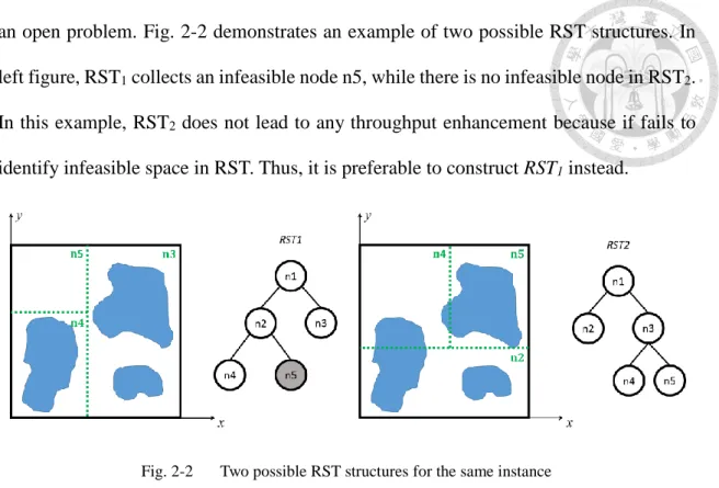
an open problem. Fig. 2-2 demonstrates an example of two possible RST structures. In left figure, RST1 collects an infeasible node n5, while there is no infeasible node in RST2. In this example, RST2 does not lead to any throughput enhancement because if fails to identify infeasible space in RST. Thus, it is preferable to construct RST1 instead.
Fig. 2-2 Two possible RST structures for the same instance
In this thesis, we concentrate on identifying more infeasible space because it’s the key to improve throughput. Therefore, the way to construct a RST is of our interest. In RSSDE, several heuristics were proposed. They are explained as follows.
Branch Variable Selection
In [4], they proposed a complexity level (CL) heuristic to determine the branch variable first. The CL heuristic assigns different scores to different semantic operators. The priority for operators is ordered by (5).
CL(EQ) ≫ CL(DIV or MUL) > 𝐶𝐿(𝐴𝐷𝐷 𝑜𝑟 𝑆𝑈𝐵) > 𝐶𝐿(𝐿𝑜𝑔𝑖𝑐)
> 𝐶𝐿(𝐿𝑒𝑠𝑠𝑇ℎ𝑎𝑛 𝑜𝑟 𝑁𝐸𝑄) (5)
Suppose CL(ADD) = 10, CL(Logic) = 3, and CL(LessThan or GreaterThan) = 1.
Given three input constraints with 𝑐1: 𝑥1 + 𝑥2 ≤ 𝑥3 , c2: (𝑥1 & 𝑥2) ≥ 𝑥4 and 𝑐3: 𝑥3 ≤ 𝑥4, the complexity level of each input variable is evaluated by (6).
14
CL(𝑥𝑖) = ∑ ∑ 𝐶𝐿(𝑜𝑝)
𝑜𝑝∈𝐶𝑗 𝑖𝑓𝑥𝑖∈𝐶𝑗 𝑚
𝑗=1 (6)
The complexity level scores for x1, x2, x3 and x4 are CL(x1) = 10+1+3+1 = 15, CL(x2) = 10+1+3+1 = 15, CL(x3) = 10+1+1 = 12 and CL(x4) = 3+1+1 = 5 respectively. Thus, the priority order for selecting the branch variable is 𝑥1 = 𝑥2 >
𝑥3 > 𝑥4.
Cutting Plane Selection
After branch variable is determined, we need to decide the cutting plane position.
Three heuristics were proposed to decide cutting plane position.
1. Bisection
This approach splits at the mid-point of the feasible range of selected branch variable.
2. Constraint-based
Some special constraint types are supported by this method. Once the supported constraint is recognized, cutting plane positions are automatically determined. For example, it supports constraint like ∑𝑥𝑖 ≤ 𝑐𝑜𝑛𝑠𝑡. Cutting plane decision for each variable is automatically positioned at ⌊𝑐𝑜𝑛𝑠𝑡𝑁 ⌋ + 1, where N is the number of input variables appeared in that constraint.
3. Split-on-demand
This method applies some random samples first and utilizes feasible samples to guide cutting plane decision. Regions without feasible samples are cut at their boundaries.
15
However, there are some possible drawbacks of previous approaches outlined as follows.
1) In some situations, bisection method requires more nodes in RST to identify the same amount of infeasible space.
2) Constraint based method is applicable to only special types of constraints.
3) If the original solution density is extremely low, split-on-demand approach may need vast amounts of random samples to guide cutting plane decision. For instance, if we need 100 feasible samples to determine one cutting plane position, an internal node with solution density of 10-4 needs total 106 random samples for such decision.
2.3 RST Guided Pattern Generation Stage
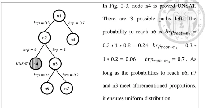
Fig. 2-3 illustrates how to use the RST to guide pattern generation. Each internal edge is annotated with branching probability brp. The value of brp is determined by the proportion of the number of feasible patterns in each sub-space. For example, 𝑏𝑟𝑝𝑛1→𝑛2= 0.3 and 𝑏𝑟𝑝𝑛1→𝑛3= 0.7 means the ratio between the number of feasible solutions in n2 and n3 is 3:7. There are four leaf nodes n3, n4, n6 and n7 in Fig. 2-3. Node n4 is proved infeasible by the formal technique. The probability to reach each feasible leaf node is the product of branch probabilities along the path of top-down random walk.
16
In Fig. 2-3, node n4 is proved UNSAT.
There are 3 possible paths left. The probability to reach n6 is 𝑏𝑟𝑝𝑟𝑜𝑜𝑡→𝑛6 = 0.3 ∗ 1 ∗ 0.8 = 0.24 𝑏𝑟𝑝𝑟𝑜𝑜𝑡→𝑛7 = 0.3 ∗ 1 ∗ 0.2 = 0.06 𝑏𝑟𝑝𝑟𝑜𝑜𝑡→𝑛3 = 0.7 . As long as the probabilities to reach n6, n7 and n3 meet aforementioned proportions, it ensures uniform distribution.
Fig. 2-3 An example of top-down random walking in RST
2.4 RSSDE Algorithm
(a) (b)
Fig. 2-4 (a) Shows the entire solution space of x + y < 6 or x > y + 6 with 0 ≤ x, y ≤ 10 (b) Shows one possible RST structure. (Modified from [12])
Fig. 2-4 demonstrates another example. In (b), it is one possible RST structure corresponding to (a). There are two reachable leaf nodes n4 and n7. The solution densities are annotated on the nodes in RST. Both nodes n4 (58.33%) and n7 (50%) have higher
17
solution densities than root (25.6%). This is not always the case. Some leaf nodes may possibly have less solution densities after RST construction. However, as we prune more infeasible space in RST, leaf nodes in general have higher solution densities.
Discussion of Low Solution Density Nodes of RST
It is worth noting that after RST construction, some leaf nodes may still have extremely low solution density. For such hard-to-hit regions, applying A&R is time- consuming and thus SAT based techniques [3][8] are suggested to be used. SAT-based patterns generated in these regions actually bias the uniform distribution. However, if the probabilities to reach these regions keep low, RSSDE can still ensure (near) evenness in a macro view.
Fig. 2-5 illustrates the overall RSSDE algorithm. In this thesis, we focus on developing an alternative way of RST construction at line 14 and 15.
18
Algorithm 1 Pseudocode of the RSSDE algorithm
Input: confidence level (cl), max interval (w), max ratio (γ) and threshold size of
ℛ𝑆𝑇 (T)Output: an RS-tree (ℛ𝑆𝑇)
1. Let queue store to-be-split nodes.
2. Let hr be the observed hit-rate
3. Let var be the branch variable and vs be its splitting point
4. Let node represent one node in ℛ𝑆𝑇. Its child nodes are denoted as left and right.
5. begin
6. ℛ𝑆𝑇 = initDistributionTree() 7. queue.push( ℛ𝑆𝑇.root )
8. while queue is not empty and tree size is less than T begin 9. node = queue.pop()
10. hr = random_sampling(node, ci, w, γ)
11. if hr is zero and prove (node) is INFEASIBLE begin 12. markInfeasible(node);
13. end else if hr satisfies branching condition begin 14. var = selectBranchVariable()
15. vs = genSplitValue(var)
16. (left, right) = branch(ℛ𝑆𝑇, node, var, vs) 17. queue.push( left )
18. queue.push( right ) 19. end
20. end
21. return ℛ𝑆𝑇 22. end
Fig. 2-5 The RSSDE algorithm [4]
19
Chapter 3 Global and Local Infeasible Space Identification
To enhance throughput of RSSDE, the ability to identify infeasible space is the key.
We first categorize input variables into two groups.
Definition 1 (Universally reducible variables)
An input variable 𝑥𝑖 is called universally reducible if there exists an interval γ of 𝑥𝑖, such that a random assignment 𝑣𝑖 ∈ 𝛾 of 𝑥𝑖 is sufficient to make the constraints UNSAT. In Example 3-1, x1, x2 and x3 are all universally reducible variables because any assignment of 𝑣𝑥1 ∈ 𝛾𝑥1 = [100: 900] 𝒐𝒓 𝑣𝑥2 ∈ 𝛾𝑥2= [300: 700] 𝒐𝒓 𝑣𝑥3∈ 𝛾𝑥3 = [500: 800] makes the constraints infeasible.
Example 3-1): Four input variables with initial range of [0:1023] and 3 input constraints 𝑐1: 100 < 𝑥1 𝑜𝑟 𝑥1 > 900, 𝑐2: 𝑥2 < 300 𝑜𝑟 𝑥2 > 700 𝑎𝑛𝑑 𝑐3: 500 < 𝑥3 𝑜𝑟 𝑥3 >
800.
Definition 2 (Conditionally reducible variables)
An input variable 𝑥𝑖 is called conditionally reducible if there exists an interval 𝛾𝑖 of 𝑥𝑖, such that a random assignment 𝑣𝑖 ∈ 𝛾 of 𝑥𝑖 makes the constraints POSSIBLY UNSAT. In other words, its infeasibility also depends on the assignments of the other variables. In Example 3-2, x1 and x2 are both conditionally reducible variables.
Constraints fail when 𝑣𝑥1 ∈ 𝛾𝑥1 = [512: 1023] 𝒂𝒏𝒅 𝑣𝑥2 ∈ 𝛾𝑥2 = [512: 1023]. If only 𝑣𝑥1 ∈ 𝛾𝑥1 = [512: 1023], it is not sufficient to deduce the infeasibility. It must also consider the value assignment of x2 at the same time.
20
Example 3-2): There are two input variables x1 and x2 with initial range of [0:1023] and one constraint 𝑐1: 𝑥1 + 𝑥2 < 1024.
Due to the observation above, we propose two-stage infeasible space identification technique. Global infeasible space identification is followed by local infeasible space identification stage. Global identification stage focuses on pruning the ranges of universally reducible variables, while local identification stage concentrates on pruning infeasible space resulted from conditionally reducible variables.
In general speaking, universally reducible variables usually contribute to higher proportion of infeasible space. It can be seen as a coarse pruning technique. In the opposite, pruning on conditionally reducible variables normally results in tuning on finer infeasible space. Reducing the ranges of universally reducible variables in advance does not impact on uniform property. Thus, we try to prune universally reducible variables as more as we can at global identification stage since it helps to eliminate unnecessary nodes of RST. Unlike universally reducible variables, pruning infeasible space composed of conditionally reducible variables is easily resulted in biased distribution (just like interval-propagation). RST comes in handy in this situation because it still keeps uniform distribution by annotating branch probabilities in each path. Although it is fairly trivial in Example 3-1. However in general cases, universally reducible variables are not easy to detect for complex and intertwined constraints.
The difference between our approach and RSSDE is shown in Fig. 3-1. In original RSSDE, although they apply simple word-level analysis before RST construction, their analysis are limited to simple constraint format only. They do not consider the dependencies across multiple constraints. In our approach, we take these dependencies into account. Our inference is strongly based on the formal engine. Because of the
21
completeness of formal engine, our approach can effectively prune more infeasible ranges of universally reducible variables. In short, we are particularly interested in extracting most (nearly-all) of the infeasible ranges of universally reducible variables before RST construction. The benefits of this approach is demonstrated in the next sub-section. After global identification stage, infeasible space composed of conditionally reducible variables are recognized by the help of RST. In our experience, by separating these two kinds of variables into two groups and applying different approaches to each of them, we can effectively identify more infeasible space. The overall throughput thus can be substantially enhanced, especially for those hard constraints with lots of universally reducible variables resulted from dependencies of complex constraints.
Fig. 3-1 Proposed approach versus original approach
3.1 Applicability of Global and Local Infeasible Space Identification
Observation 3-1): RST is adequate for conditionally reducible variables, but NOT for
universally reducible variables.22
In essence, RST is a range splitting tree. It recursively partitions solution space into multiple disjoint sub-space. Each leaf node can be seen as the cofactor sub-space of input variables on the path from root to the leaf node. Although we can also use RST to identify universally reducible variables, but it requires more nodes in RST to prune the same amount infeasible space without shrinking universally reducible variables in advance.
This phenomenon is demonstrated in Fig. 3-2. Fig. 3-2 illustrates one of possible RST structure for Example 3-1. In Fig. 3-2, if we want to shrink the range of universally reducible variables in RST, we need to split on EVERY possible path in RST. Variables
x2 in depth 2 and x3 in depth 3 show such situation. If we have many universally reducible
variables, the size of RST quickly increases. Fig. 3-3 is an extension of Fig. 3-2 for Example 3-3.Fig. 3-2 A possible RST structure for Example 3-1
Example 3-3): Extended from Example 3-1, suppose there is a new input variable x4 and a new constraint 𝑐4: 𝑥4 < 𝑥1. Fig. 3-3 depicts the new RST structure extended from the RST structure of Fig. 3-2. There are total 12 feasible leaf nodes of the resulted RST.
23
Fig. 3-3 An extended RST structure from Fig. 3-2.
We can mitigate this node explosion problem by identifying universally reducible variables before RST construction. Fig. 3-4 shows a smaller RST by applying global infeasible space identification first. Reduced feasible ranges are denoted on the root node.
If we need to extract same amount of infeasible space without reducing initial ranges in RST, we need to construct a larger RST. This example is trivial and should be able to deduce from the constraints directly. In our work, we focus on universally reducible variables resulted from the dependency of MULTIPLE constraints. Complex and intertwined constraints are not so obvious to deduce such variables by just using simple word-level analysis. We show this in Example 3-4.
24
Fig. 3-4 A smaller RST structure by applying global infeasible space identification first.
Example 3-4): Given two input variables x1, x2 with initial ranges [1:1000] and two constraints 𝑐1: 𝑥1 ∗ 𝑥2 ≤ 1000 and 𝑐2: 𝑥1 ≥ 𝑥2.
Consider if we apply a direct interval propagation method for Example 3-4, we cannot reduce the feasible range of x2 from [1:1000] to [1:31] as shown in Fig. 3-5. In this case, we know that x2 is an universally reducible variable and is be able to perform initial range reduction beforehand. However, a naïve interval propagation fails to conclude such reduction. In Fig. 3-5 (a), the backward implication on node “≤” implies
“MUL” node with feasible range [1:1000]. Then, a recursive backward implication on
“MUL” node derives feasible ranges [1:1000] of x1 and x2 which are identical for the original ranges of x1 and x2. Similarly, in Fig. (b), inference on node “≥” indicates the feasible range is [1:1000] for both x1 and x2. There is no further range reduction in forward implication. The entire implication finishes at this step.
25
(a) Backward implication on “≤” node (b) Backward implication on “≥” node
Fig. 3-5 Naïve interval propagation does not further reduce range of x2.
At global identification stage, we make extensive use of state-of-the-art SMT solver, boolector. Boolector itself already implemented many word-level optimizations in bit- vector arithmetic logic, which is suitable for evaluation of our approach. We use it as a black-box and try to reduce the burdens of SMT proofs. Our approach does not need complex implication engine and thus is fairly easy to implement. Our experimental evaluations show the efficiency of SMT solver in our approach to prune universally reducible variables. Although we cannot extract all the infeasible space composed of universally reducible variables unless a brute-force technique is applied. We still can extract most part of it, and remaining infeasible space comprised of conditionally reducible variables can be further identified by utilizing RST technique.
Observation 3-2): Nodes closer to the root occupy a larger proportion of original space.
From Observation 3-2, it is usually better to prune infeasible space with nodes closer to the root as it occupies larger part of the search space. Consider using pure bisection
26
method for RST construction, an infeasible node identified at the depth d contributes to (12)𝑑 percent of original search space. According to (3), we should try to collect larger infeasible space for a RST in order to increase the overall throughput.
We utilize (7) to approximate the solution density after RST construction without loss of generality.
𝑆𝑜𝑙𝑢𝑡𝑖𝑜𝑛𝐷𝑒𝑛𝑠𝑖𝑡𝑦𝑅𝑆𝑇 = ∑𝑥𝑖∈𝑓𝑒𝑎𝑠𝑖𝑏𝑙𝑒_𝑙𝑒𝑎𝑣𝑒𝑠#𝐹𝑒𝑎𝑠𝑖𝑏𝑙𝑒𝑃𝑎𝑡𝑡𝑒𝑟𝑛𝑠𝑥𝑖
∑𝑥𝑖∈𝑓𝑒𝑎𝑠𝑖𝑏𝑙𝑒_𝑙𝑒𝑎𝑣𝑒𝑠𝐻𝑦𝑝𝑒𝑟𝑉𝑜𝑙𝑢𝑚𝑒𝑥𝑖 (7)
Example 3-5): Assume solution density of original search space is 10−4. After RST construction, the total amount of identified infeasible volume in RST occupies 50%. The overall solution density for the RST can be approximated as 2 ∗ 10−4.
In the following subsections, we will explain our global and local infeasible space identification methods in details.
27
3.2 Global Infeasible Space Identification
This stage focuses on identifying universally reducible variables only. We don’t apply split-on-demand method because in our experience, if the solution density is lower than a threshold, before we collect enough feasible samples, we already waste lots of random samples in infeasible space. In addition, there may exist feasible but not sampled points by using random sampling. Without successfully sampling those feasible points, we can be misguided by deriving an incorrect splitting position. Fig. 3-6 depicts such situation, interval [a, d] of x may be considered as an infeasible interval by using only sampled feasible points. However, dotted points represent the feasible but not sampled solutions. In this case, interval [b, c] of x is the valid infeasible interval while interval [a,
d] is not. Thus, for split-on-demand method, false positives may occur when the solution
density is extremely low or number of variables is large. If the number of variables is large, the combinations of value assignments for all variables are also huge. Exact random sampling in each projection is not practical. Besides, some may wonder to apply smoothing to overcome such issue. However, bitwise operators make it difficult as them usually result in many non-contiguous feasible sub-ranges. In our approach, we give up using split-on-demand method to derive cutting plane positions. Instead, we resort to formal SMT engine directly. SAT versus SMT
The reason we choose to use “word-level” (SMT) solver rather than its “boolean-
level” counterpart (SAT) is because in CRV, inputs are limited to integer variables.
This actually fits the quantifier-free bit-vector (QF-BV) arithmetic logic of SMT theory. A SAT solver [14] operates on binary variables, which loses high level
28
inference capability. A SAT solver needs to use extra time just to learn simple word- level implication from binary variables. For example, given three 32-bit variables A,
B, and C. Constraints with
𝐴 < 𝐵 && 𝐵 < 𝐶 → 𝐴 < 𝐶 requires more implications and decision steps in pure SAT reasoning.Fig. 3-6 An illustration of feasible but not sampled points
3.2.1 Brute-Force Approach
This method divides the initial range γ of each input variable into len(γ) unit- length intervals. Then, each unit-length interval is checked with feasibility by applying the SMT solver. This brute-force approach can prune ALL infeasible space composed of universally reducible variables. However, it requires total 𝑁 ∗ 2𝑀 of SMT proofs for the problem of N input variables with feasible bit-width M. This is very time-consuming.
3.2.2 Depth-Limited Bisection Approach (Single SMT instance)
Brute-force approach suffers from runtime efficiency. In this approach, we propose a depth limited bisection method to accelerate such procedure. The intuition is that even for complex and intertwined constraints, there may exist many input variables which are
29
not universally reducible. For such variables, we can perform an early exist instead of repeatedly applying SMT engine to each possible sub-interval. This approach defines a pre-determined parameter limit. It recursively splits the original range of each input variable and uses SMT solver to prove feasibility of each interval. If we cannot find any infeasible interval within depth limit, we recognize current variable as non-universally reducible. We give up further splitting for such variable. Otherwise, variable with any infeasible interval found within depth limit is regarded as universally reducible. We keep further splitting that variable until unit-length interval is derived. Fig. 3-7 illustrates the detailed procedure. Two queue structures are used to store ranges and depths respectively.
At line 18, is_reducible is marked TRUE if an infeasible interval can be found with depth
limit.
Example 3-6): Consider three input variables x1, x2 and x3 with initial ranges [0:1023]
and three input constraints 𝑐1: 𝑥1 ∗ 𝑥2 < 1024, 𝑐2: 𝑥1 ≥ 𝑥2 and 𝑐3: 𝑥1 ≥ 𝑥3. Suppose that limit is 5, initial range [0:1023] of x1 will be checked by SMT at depth 0. If the range is proved feasible, it splits at the mid point (0+10232 = 511) and pushes two sub-ranges [0:511] and [512:1023] into the queue. This process continues until the queue is empty.
If any of the range is proved infeasible within depth less than 5, this variable will be marked as reducible. And the splitting process will only be terminated in the unit-length interval. Otherwise, the process terminates at exact depth 5. This approach guarantees every contiguous infeasible interval whose length equal and larger than 10242𝑑 will be detected. Above steps are repeated until all variables are exhausted (x2 and x3).
30
Depth-limited Bisection Approach
Input: input variable var and input constraints C, predefined depth limit Output: Reduced input variable var’
1. Let queue store disjoint ranges of an input variable.
2. Let queue_depth store corresponding depths of the nodes in queue.
3. Let range be the range of the current split node.
4. Let range_left and range_right be two disjoint sub-ranges of range.
5. Let depth be the depth of the current split node.
6. Let feasible_ranges store reduced ranges of an input variable.
7. begin
8. queue.push( initalRange(var) ); queue_depth.push(0) 9. is_reducible = FALSE
10. While queue is not empty begin
11. range = queue.pop(); depth = queue_depth.pop()
12. if (range.min == range.max or (depth > limit & is_reducible == FALSE)) 13. begin
14. feasible_ranges = storeFeasibleRanges(range) 15. Continue
16. end
17. if prove(range) is Infeasible 18. is_reducible = TRUE 19. else begin
20. (range_left, range_right) = bisectAtMidPoint(range, queue) 21. queue.push(range_left); queue.push(range_right)
22. queue_depth.push(depth + 1); queue_depth.push(depth + 1) 23. end
24. end
25. if is_reducible == TRUE
26. var’ = replaceOrgRanges(var, feasible_ranges) 27. end
Fig. 3-7 The depth-limited bisection approach
31
3.2.3 Iterative Event-Driven Approach (Multiple STM instances)
In previous two approaches, ONE SMT instance is built for the whole constraint set.
In this section, we propose an alternative iterative event-driven approach. Instead of creating a single SMT instance to prove the whole constraint set, we create multiple SMT instances. Each SMT instance handles for partial constraint set. By dividing a large constraint set into several smaller ones, we make SMT reasoning procedure much easier for each smaller instance. However, false positives may exist for this modification. A variable which is proved full-range feasible by a single SMT instance can actually be wrong. We demonstrate this approach in Example 3-7.
Example 3-7): Give three input variables x1, x2, x3 with initial ranges [0:1023] and three constraints 𝑐1: 𝑥1 ∗ 𝑥2 ≤ 1000, 𝑐2: 𝑥1 ≥ 𝑥2 and 𝑐3: 𝑥2 ≥ 𝑥3.
First, we create individual SMT instance for each variable. We use the subscript as the representative variable notation for SMT instances. In this example, three SMT instances SMTx1, SMTx2 and SMTx3 will be created. Variables x1, x2 and x3 are representative variables for SMTx1, SMTx2 and SMTx3 respectively. In this method, we always create N SMT instances given N input variables. For SMTx1, it is constructed for constraint set {c1, c2} and variable set {x1, x2}. Similarly, for SMTx2, it includes the constraint set {c1, c2, c3} and variable set {x1, x2, x3}, and SMTx3 contains constraint set {c3} and variable set {x2, x3} as shown in Fig. 3-8. For each individual SMT instance, we apply depth-limited approach as previously described. Next, each SMT instance will prove the feasibility with regard to only its representative variable. That is, SMTx1,
SMTx2 and SMTx3 will prove the range-feasibility of x1, x2 and x3 respectively. After
formal SMT reasoning, we derive that variables x1 and x3 are full-range feasible fromSMTx1 and SMTx3. And SMTx2 proves that variable x2 can be reduced to a smaller range.
32
Please be noted that if we finish the procedure at this step. Variable x3 would not be recognized as reducible. The reason is resulted from the construction of partial set for
SMTx3. Since SMTx3 only includes constraint set {c3} and variables set {x2, x3}. The
initial range is [0:1023] for x2 and x3. Thus, we cannot reduce initial range [0:1023] ofx2 and x3 by SMTx3 at the beginning. However, for SMTx2, it indeed shrinks the feasible
range of variable x2. As long as this reduction information of x2 can be transmitted toSMTx3, variable x3 can be further reduced by SMTx3 as well.
This is how we come up with iterative approach here. Whenever a representative variable is proved reducible by its own SMT instance, it triggers a new iteration for all related SMT instances of that variable. In this example, variable x2 will be related to
SMTx1, SMTx2 and SMTx3 because variables x1, x2, and x3 all appear in the constraint
set of SMTx2. We add these three SMTx1, SMTx2, SMTx3 instances for the next iteration and re-verify new SMT instances in queues and add a new constraint restricting the feasibility range of x2 in each SMT instance. Suppose at the first run, the feasible range of x2 is proven within range [0:127], we will add the constraint 𝐶𝑛𝑒𝑤: 0 ≤ 𝑥2 ≤ 127 toSMTx1, SMTx2 and SMTx3 before next iteration. After the second run of SMT proof, the
range of x3 is now reduced to [0:127] and x2 can also be further reduced to a smaller range.33
Fig. 3-8 An example of multiple SMT instances
Above procedure terminates when the queue is empty which means there is no new event issuing from detecting a reducible variable. In addition, we can set up a pre- determined parameter iteration_limit to perform early exit. Luckily, in our experience, such convergence is done in just a few iterations. The intuition behind this is by partitioning whole constraint set into smaller ones, even though this creates more (exactly
N) smaller SMT instances for N input variables, each individual SMT instance is now far
more easier for reasoning. The false positives are eliminated by recurring iterations. The detailed algorithm is shown in Fig. 3-9.
34
Iterative Event-Driven Algorithm
Input: input variables X and input constraints C, predefined iterative limit K Output: range-reduced input variable X’
1. Let cur_smt_events, nxt_smt_events store to-be-proved SMT instance queues of current and next iterations.
2. Let SMTxi be a single SMT instance with representative variable xi 3. Let VarSetxi store all the input variables in SMTxi
4. begin
5. Foreach xi in X begin 6. Construct SMTxi for xi
7. Add SMTxi instance into cur_smt_events 8. end
9. For i = 0 to K begin 10. nxt_smt_events.clear()
11. While cur_smt_events is not empty begin 12. SMTxi
= cur_smt_events.pop()
13. if xi of SMTxi is proved reducible begin 14. Extract related input variables VarSetxi of xi 15. Foreach var in VarSetxi
begin
16. if SMTvar
is not in nxt_smt_events begin
17. Add SMTvar instance into nxt_smt_events 18. end19. Add new range constraint of xi into SMTvar
20. end
21. update the feasible range of xi 22. end
23. end
24. cur_smt_events = nxt_smt_events 25. end
26. end
Fig. 3-9 The iterative event-driven approach
35
At line 6, we create an individual SMT instance for each input variable and push them into the current event queue. The iterative count is limited by predefined iteration limit K. Next, each input variable xi is checked with feasibility of the range by its corresponding instance SMTxi. If xi is reducible, we extract related input variables of xi called VarSetxi. In Example 3-7, VarSetx1, VarSetx2, VarSetx3 are {x1, x2}, {x1, x2, x3}, {x2,

![Fig. 2-5 The RSSDE algorithm [4]](https://thumb-ap.123doks.com/thumbv2/9libinfo/9603325.629706/30.892.135.788.115.267/fig-the-rssde-algorithm.webp)