5 Supervised Classification

(1)

89

5 Supervised Classification

5.1 Introduction

Supervised learning is a very popular approach in any text classification task. Many different algorithms are available that learn classification patterns from a set of labeled or classified examples. Given this sample of examples, the task is to model the classification process and to use the model to predict the classes of new, previously unseen examples. In information retrieval the supervised techniques are very popular for the classification of documents into subject categories (e.g., the classification of news into financial, political, cultural, sports, …) using the words of a document as main features. In information extraction usually smaller content units are classified with a variety of classification schemes ranging from rather generic categories such as generic semantic roles of sentence constituents to very specific classes such as the number of heavily burned people in a firework accident.

As in text categorization, the amount of training examples is often lim- ited, or training examples are expensive to build. When the example set is small, it very often represents incomplete knowledge about the classification model sought. This danger is especially present in natural language data where a large variety of patterns express the same content.

Parallel to text categorization, the amount of different features is large and the feature set could include some noisy features. There are many different words, syntactic, semantic and discourse patterns that make up the context of an information element. But, compared to text categorization lesser features in the context are indicative of the class sought. Often, the features behave dependently and the dependency is not always restricted to co-occurrence of certain feature values, it sometimes also demands that feature values occur in a certain order in the text. When different classes are to be assigned to text constituents, the class assignment might also be dependent on classes previously assigned.

(2)

90 5 Supervised Classification

approaches that have been used to extract information from text and relevant references were cited. In this chapter we dig deeper into the current and most successful algorithms for information extraction that use a super- vised learning approach. The chosen classifiers allow dealing with incom- plete data and with a large set of features that on occasion might be noisy.

They also have the potential to be used for weakly supervised learning (described in the next chapter), and incorporate dependencies in their models.

As seen in Chap. 4 a feature vector x is described by a number of fea- tures (see Eq. (4.1)) that may refer to the information element to be classified, to the close context of the element, to the more global context of the document in which the element occurs, and perhaps to the context of the document collection. The goal is to assign a label y to a new example.

Among the statistical learning techniques a distinction is often made be-

model of the joint probability, p(x(( ,y) and makes its predictions by using Bayes’ rule to calculate p(y x)¹and then selects the most likely label y. An example of a generative classifier that we will discuss in this chapter is a hidden Markov model. A discriminative classifier models the posterior r probability p(y x) directly and selects the most likely label x y, or learns a di- rect map from inputs x to the class labels. An example is the maximum en- tropy model, which is very often used in information extraction. Here, the joint probability p(x(( ,y) is modeled directly from the inputs x. Another ex- ample is a Support Vector Machine, which is a quite popular learning technique for information extraction. Some of the classifiers adhere to the maximum entropy principle. This principle states that, when we make in- ferences based on incomplete information, we should draw them from that probability distribution that has the maximum entropy permitted by the in- to this principle. They are the maximum entropy model and conditional random fields.

In information extraction sometimes a relation exists between the various classes. In such cases it is valuable not to classify a feature vector separately from other feature vectors in order to obtain a more accurate

1With a slight abuse in notation in the discussion of the probabilistic classifiers, we will also use p(y(( x) to denote the entire conditional probability distribution provided by the model, with the interpretation that y and x are placeholders rather than specific instantiations. A model p(y x) is an element of all conditional prob-x ability distributions. In the case that feature vectors take only discrete values, we will denote the probabilities by the capitalized letter P.

dan, 2002). Given inputs x and their labels y, a generative classifierr learns a tween generative and discriminative classifiers (Vapnik, 1988; Ng and Jor-

formation we have (Jaynes, 1982). Two of the discussed classifiers adhere Chap. 2 gave an extensive historical overview of machine learning

(3)

9

classification of the individual extracted information. This is referred to as context-dependent classification as opposed to context-free classification.

So, the class to which a feature vector is assigned depends on 1) the feature vector itself; 2) the values of other feature vectors; and 3) the existing relation among the various classes. In information extraction, dependencies exist at the level of descriptive features and at the level of classes, the latter also referring to classes that can be grouped in higher-level concepts (e.g., scripts such as a bank robbery script). We study two context-dependent classifiers, namely a hidden Markov model and one based on conditional random fields.

Learning techniques that present the learned patterns in representations that are well conceivable and interpretable by humans are still popular in information extraction. Rule and tree learning is the oldest of such ap- proaches. When the rules learned are represented in logical propositions or first-order predicate logic, this form of learning is often called inductive logic programming (ILP). The term relational learning refers to learning in any format that represents relations, including, but not limited to logic programs, graph representations, probabilistic networks, etc. In the last two sections of this chapter we study respectively rule and tree learning, and relational learning.

The selection of classifiers in this chapter by no means excludes other supervised learning algorithms for which we refer to Mitchell (1997) and Theodoridis and Koutroumbas (2003) for a comprehensive overview of the supervised classification techniques.

When a binary classifier is learned in an information extraction task, we are usually confronted with an unbalanced example set, i.e., there are usu- ally too many negative examples as compared to the positive examples.

Here techniques of active learning discussed in the next chapter might be of help to select a subset of negative examples.

When using binary classification methods such as a Support Vector Machine, we are usually confronted with the multi-class problem. The lar- ger the number of classes the more classifiers need to be trained and applied. We can handle the multi-class problem by using a one-vs-rest (one class versus all other classes) method or a pair wise method (one class versus another class). Both methods construct multi-class SVMs by combining several binary SVMs. When classes are not mutually exclusive, the one-vs-rest approach is advisable.

In information extraction we are usually confronted with a complex problem. For instance, on one hand there is the detection of the boundaries of the information unit in the text. On the other hand there is the classification of the information unit. One can tackle these problems separately, or learn and test the extractor in one run. Sometimes the semantic classes to 5.1 Introduction 91

(4)

be assigned are hierarchically structured. This is often the case for entities to be recognized in biomedical texts. The hierarchical structure can be exploited both in an efficient training and testing of the classifier by assum- ing that one class is subsumed by the other. As an alternative, in relational learning one can learn class assignment and relations between classes. A similar situation occurs where components of a class and their chronologi- cal order signal a superclass. An important motivation for separating the classification tasks is when they use a different feature set. For instance, with the boundary recognition task, the orthographic features are impor-

will be tackled in Chap. 10.

5.2 Support Vector Machines

Early machine learning algorithms aimed at learning representations of simple symbolic functions that could be understood and verified by ex- perts. Hence, the goal of learning in this paradigm was to output a hypothesis that performed the correct classification of the training data, and the learning algorithms were designed to find such an accurate fit to the data. The hypothesis is complete when it covers all positive examples, and it is consistent when it does not cover any negative ones. It is possible that t a hypothesis does not converge to a (nearly) complete and (nearly) consistent one, indicating that there is no rule that discriminates between the positive and the negative examples. This can occur either for noisy data, or in case where the rule language is not sufficiently complex to represent the dichotomy between positive and negative examples.

This situation has fed the interest in learning a mathematical function that discriminates the classes in the training data. Among these, linear functions are the best understood and the easiest to apply. Traditional statistics and neural network technology have developed many methods for discriminating between two classes of instances using linear functions.

They can be called linear learning machines as they use hypotheses that form linear combinations of the input variables.

In general, complex real-world applications require more expressive hypothesis spaces than the ones formed by linear functions (Minsky issue of separating the learning tasks or combining them in one classifier tant, while in the classification task the context words are valuable. The

alternative solution by mapping the data into a high dimensional feature abstract features of the data are exploited. Kernel representations offer an a simple linear combination of the given features, but requires that more and Papert, 1969). Frequently, the target concept cannot be expressed as

(5)

5.2 Support Vector Machines 93

space where a linear separation of the data becomes easier. In natural language classification, it is often not easy to find a complete and consistent hypothesis that fits the training data. And in some cases linear functions are insufficient in order to discriminate the examples of two classes. This is because natural language is full of exceptions and ambiguities. We may not capture sufficient training data, or the training data might be noisy in order to cope with these phenomena, or the function we are trying to learn does not have a simple logical representation.

In this section we will lay out the principles of a Support Vector Ma- chine for data that are linearly or nearly linearly separable. We will also introduce kernel methods because we think they are a suitable technology for certain information extraction tasks.

The technique of Support Vector Machines (Cristianini and Shawe- two classes. In information extraction tasks the two classes are often the positive and negative examples of a class. In the theory discussed below we will use the terms positive and negative examples. This does not ex- clude that any two different semantic classes can be discriminated.

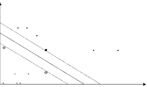
Fig. 5.1. A maximal margin hyperplane with its support vectors highlighted (after rable and then generalize the idea to data that are not necessarily linearly separable and to examples that cannot be represented by linear decision surfaces, which leads us to the use of kernel functions.

We will first discuss the technique for example data that are linearly sepa- Taylor, 2000) is a method that finds a function that discriminates between

Christianini and Shawe-Taylor, 2000).

(6)

In a classical linear discriminant analysis, we find a linear combination of the features (variables) that forms the hyperplane that discriminates between the two classes (e.g., line in a two-dimensional feature space, plane in a three-dimensional feature space). Generally, many different hyperplanes exist that separate the examples of the training set in positive and negative examples among which the best one should be chosen. For instance, one can choose the hyperplane that realizes the maximum margin between the positive and negative examples. The hope is that this leads to a better generalization performance on unseen examples. Or in other words, the hyperplane with the margin d that has the maximum Euclidean d distance to the closest training examples (support vectors) is chosen. More formally, we compute this hyperplane as follows:

Given the set S of n training examples:

S= {(x¹, y¹),...,(xⁿ, yⁿ)}

where xi∈ℜℜ^p^p⁽(( -dimensional space) and y^p i∈ {–1,+1} indicating that xⁱis respectively a negative or a positive example.

When we train with data that are linearly separable, it is assumed that some hyperplane exists which separates the positive from the negative examples. The points which lie on this hyperplane satisfy:

w⋅ xⁱ + b = 0 (5.1) where w defines the direction perpendicular to the hyperplane (normal to the hyperplane). Varying the value of b moves the hyperplane parallel to itself. The quantities w and b are generally referred to as respectively weight vector and r bias. The perpendicular distance from the hyperplane to the origin is measured by:

b

w (5.2) where w is the Euclidean norm of w.

Let d+(d-) be the shortest distance from the separating hyperplane to the closest positive (negative) example. d+and d-thus define the margin to the hyperplane. The task is now to find the hyperplane with the largest margin.

Given the training data that are linearly separable and that satisfy the following constraints:

(7)

w⋅ xⁱ + b ≥ +1 for yi= +1 (5.3)

w⋅ xⁱ + b ≤ −1 for yi= 1 (5.4) which can be combined in 1 set of inequalities:

yi( w⋅ xⁱ + b) −1 ≥ 0 for i = 1,…, n (5.5) The hyperplane that defines one margin is defined by:

H¹: w⋅ xⁱ + b =1 (5.6) with perpendicular distance from the origin:

1− b

w (5.7)

The hyperplane that defines the other margin is defined by:

H²: w⋅ xⁱ + b = −1 (5.8) with perpendicular distance from the origin:

−1− b

w (5.9)

Hence d+= d-= 1

w and the margin = 2 w ^.

In order to maximize the margin the following objective function is computed:

Minimize_w,b w⋅w

Subject to yⁱ( w⋅ xⁱ + b) −1 ≥ 0, i =1,...,n (5.10)

−

(8)

Linear learning machines can be expressed in a dual representation, which turns out to be easier to solve than the primal problem since handling ine- quality constraints directly is difficult. The dual problem is obtained by in- troducing Lagrange multipliers λλⁱ, also called dual variables. We can transform the primal representation into a dual one by setting to zero the derivatives of the Lagrangian with respect to the primal variables, and substituting the relations that are obtained in this way back into the La-

Maximize W (λλλ⁾= λλλⁱ

i=1 n

¦

⁻¹₂ ^λ^{λλ λ}ⁱ^λλ^j^{jj i}^y^{i j}^y^{yy x}ⁱ^⋅x^x^j

i, j=1 n

¦

Subject to: λλλⁱ≥ 0 λⁱ λλ^y λ^{i i}= 0

i=1 n

¦

⁰^, i =1,...,n

(5.11)

It can be noticed that training examples only need to be inputted as inner products (see Eq. (5.11)), meaning that the hypothesis can be expressed as a linear combination of the training points. By solving a quadratic optimi- zation problem, the decision function h(x(( ) for a test instance x is derived as follows:

h(x)= sign( f (x)) (5.12)

f (x)= λλλλλλⁱⁱ^yⁱ ^xⁱ⋅ x + b

i=1 n

¦

(5.13)

The function in Eq. (5.13) only depends on the support vectors for which λi

λ > 0. Only the training examples that are support vectors influence the decision function. Also, the decision rule can be evaluated by using just inner products between the test point and the training points.

We can also train a soft margin Support Vector Machine which is able to deal with some noise, i.e., classifying examples that are linearly separable while taking into account some errors. In this case, the amount of training error is measured using slack variables ξξi, the sum of which must not exceed some upper bound.

simpler constraints:

grangian, hence removing the dependence on the primal variables. The resulting function contains only dual variables and is maximized under

(9)

The hyperplanes that define the margins are now defined as:

H¹: w⋅ xⁱ + b =1−ξξξⁱ (5.14) H²: w⋅ xⁱ + b = −1+ξξξⁱ (5.15) Hence, we assume the following objective function to maximize the margin:

Minimize

ξ , w, b w⋅w + C ξi

ξξ2

i=1 n

¦

Subject to yⁱ( w⋅ xⁱ + b) −1+ξξξ ≥ 0 , i = 1,...,nⁱ

(5.16)

where ξi

ξξ2

i=1 n

¦

= penalty for misclassification C = weighting factor.

The decision function is computed as in the case of data objects that are linearly separable (cf. Eq. (5.13)).

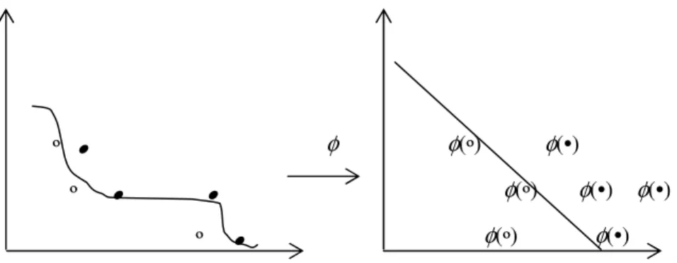
When classifying natural language data, it is not always possible to linearly separate the data. In this case we can map them into a feature space where they are linearly separable (see Fig. 5.2). However, working in a high dimensional feature space gives computational problems, as one has to work with very large vectors. In addition, there is a generalization the- ory problem (the so-called curse of dimensionality), i.e., when using too many features, we need a corresponding number of samples to insure a correct mapping between the features and the classes. However, in the dual representation the data appear only inside inner products (both in the training algorithm shown by Eq. (5.11) and in the decision function of Eq.

(5.13)). In both cases a kernel function (Eq. (5.19)) can be used in the computations.

A Support Vector Machine is a kernel based method. It chooses a kernel function that projects the data typically into a high dimensional feature space where a linear separation of the data is easier.

(10)

º • φ φφφ⁽º) φφφ^(•)

º • • φφφ⁽_º) φφφ^(•)φφφ^(•)

º • φφφ⁽_º) φφφ^(•)

Formally, a kernel function K is a mapping K: S xS S→ [0, ∞] from the instance space of training examples S to a similarity score:S

K (xⁱ,xx )^j = φφφ^k^(xⁱ⁾⁾φφφ^k^(x^{x )}^j =

k

¦

^φ^φ⁽^xⁱ⁾^⋅^φ^φ⁽^x^{x )}^j (5.17) In other words a kernel function is an inner product in some feature space (this feature space can be potentially very complex). The kernel function must be symmetric [K(KK x(( i,xx ) = K(j KK x((x ,jjjxi)] and positive semi-definite. By semi-definite we require that if x1,…,xn∈ S, then the n x n matrix G de- fined by Gij= K (K x(( i,xx ) is positive semi-definitej ²². The matrixG is called the G Gram matrix or the kernel matrix. Given G, the support vector classifier finds a hyperplane with maximum margins that separates the instances of different classes. In the decision function f(ff x) we can just replace the dot products with kernels K(KK x(( i,x,,x ).j

h(x)= sign( f (x)) (5.18) f (x)= λλλλλλⁱⁱ^yⁱφφ⁽^xⁱ⁾⋅φφ⁽^x) + b

i=1 n

¦

(5.19)

Or

f (x)= λλλλλλⁱⁱ^yⁱ^{K (x}ⁱ^,x)+ b

i=1 n

¦

2 A matrix

2 A ∈ ℜ^pxp^x is a positive semi-definite matrix if ∀∀∀x∈ℜ^px^TAx≥0. A positive semi-definite matrix has non-negative eigenvalues.

(after Christianini and Shawe-Taylor 2000).

Fig. 5.2. A mapping of the features can make the classification task more easy

(11)

To classify an unseen instance x, the classifier first projects x into the fea- ture space defined by the kernel function. Classification then consists of determining on which side of the separating hyperplane x lies. If we have a way of efficiently computing the inner product _φφ(^xⁱ⁾⋅φφ⁽^x) in the feature space as a function of the original input points, the decision rule of Eq.

(5.19) can be evaluated by at most n iterations of this process.

An example of a simple kernel function is the bag-of-words kernel used in text categorization where a document is represented by a binary vector, and each element corresponds to the presence or absence of a particular word in the document. Here, φφφk^(x⁽⁽ i) = 1 if word w occurs in document xi

and word order is not considered. Thus, the kernel function K(KK x(( i,xx ) is a j

simple function that returns the number of words in common between xi

and xx .j

Kernel methods are effective at reducing the feature engineering burden for structured objects. In natural language processing tasks, the objects being modeled are often strings, trees or other discrete structures. By calcu- lating the similarity between two such objects, kernel methods can employ dynamic programming solutions to efficiently enumerate over substruc- tures that would be too costly to explicitly include as features.

Another example that is relevant in information extraction is the tree kernel. Tree kernels constitute a particular case of more general kernels de- 2001). The idea is to split the structured object in parts and to define a kernel on the “atoms” and to recursively compute the kernel over larger parts in order to get the kernel of the whole structure.

The property of kernel methods to map complex objects in a feature space where a more easy discrimination between objects can be performed and the capability of the methods to efficiently consider the features of complex objects make them also interesting for information extraction tasks. In information extraction we can combine parse tree similarity with a similarity based on feature correspondence of the nodes of the trees. In the feature vector of each node additional attributes can be modeled (e.g., POS, general POS, entity type, entity level, WordNet hypernyms). Another example in information extraction would be to model script tree similarity of discourses where nodes store information about certain actions and their arguments.

We illustrate the use of a tree kernel in an entity relation recognition the purpose of this research is to find relations between entities that are al- ready recognized as persons, companies, locations, etc. (e.g., John works for Concentra).

fined on a discrete structure (convolution kernels) (Collins and Duffy,

task (Zalenko et al., 2003; Culotto and Sorensen, 2004). More specifically

(12)

In this example, the training set is composed of parsed sentences in which the sought relations are annotated. For each entity pair found in the same sentence, a dependency tree of this training example is captured based on the syntactic parse of the sentence. Then, a tree kernel can be defined that is used in a SVM to classify the test examples.

The kernel function incorporates two functions that consider attribute correspondence of two nodes tiand tt : A matching function m(tj i,tt )j ∈ {0, 1}

and a similarity function s(ti,tt )j ∈ [0,∞]. The former just determines whether two nodes are matchable or not, i.e., two nodes can be matched when they are of compatible type. The latter computes the correspondence of the nodes tiand tt based on a similarity function that operates on thejj

nodes’ attribute values.

For two dependency trees TT and T1 TT the tree kernel K(2 KK TT ,T1TT ) can be de-2

fined by the following recursive function:

K (tⁱ,tt )^j = 0, if m (tⁱ, tt ) = 0^j s(tⁱ,tt )^j + KKK (t^c ⁱ

[ ]

c ^,t^{t c}^j

[ ]

) otherwise

®

¯

®® (5.20)

where KKK is a kernel function that defines the similarity of the tree in terms c

of children subsequences. Note that two nodes are not matchable when one of them is nil. Let a and b be sequences of indices such that a is a sequence a1≤ a²≤ … a^kand likewise for b. Let d(a) = akk – a1 + 1 and l(a) be the length of a. Then KKK can be defined as: c

Kc

K

K (ti[c], ttj[c]) = λλλ^d^{(a )}λλλ^d^{(b )}^{K (t}ⁱ

[ ]

^a ^,t^{t b}^j

[ ]

⁾

a, b,l(a )

¦

= l(b) (5.21)

The constant 0 < λλ < 1 is a decay factor that penalizes matching subsequences that are spread out within the child sequences.

Intuitively, whenever we find a pair of matching nodes, the model searches for all matching subsequences of the children of each node. For each matching pair of nodes (s ttt ,tit ) in a matching subsequence, we accumu-j

late the result of the similarity function s(ti,tt ) and then recursively search j

for matching subsequences of their children ti[c] and tt^j[c]. Two types of tree kernels are considered in this model. A contiguous kernel only matches child subsequences that are uninterrupted by non-matching nodes.

Therefore, d(a) = l(a). On the other hand, a sparse tree kernel, allows non- matching nodes within matching subsequences.

The above example shows that kernel methods have a lot to offer in information extraction. Complex information contexts can be modeled in a

(13)

kernel function, and problem-specific kernel functions can be drafted. The problem is then concentrated on finding the suitable kernel function. The use of kernels as a general technique for using linear machines in a non- linear fashion can be exported to other learning systems (e.g., nearest neighbor classifiers).

Generally, Support Vector Machines are successfully employed in named

ognition (e.g., Zhang and Lee 2003; Mehay et al., 2005) and in entity rela- Vector Machines have the advantage that they can cope with many (sometimes) noisy features without being doomed by the curse of dimensionality.

5.3 Maximum Entropy Models

The maximum entropy model (sometimes referred to as MAXENT) com- putes the probability distribution p(x(( ,y) with maximum entropy that satisfies the constraints set by the training examples (Berger et al., 1996).

Among the possible distributions that fit the training data, the one is chosen that maximizes the entropy. The concept of entropy is known from tainty concerning an event, and from another viewpoint a measure of randomness of a message (here a feature vector).

Let us first explain the maximum entropy model with a simple example of named entity recognition. Suppose we want to model the probability of a named entity being a disease or not when it appears in three very simple contexts. In our example the contexts are composed of the word that is to be classified being one of the set {neuromuscular, Lou Gerigh, person}.

In other words, the aim is to compute the joint probability distribution p defined over {neuromuscular, Lou Gerigh, person} x {disease, nodisease}

given a training set S of nf training examples:

S = {(

S ((x, y ) , (x1 , y) ,…, (x2 (( ,y) }.n

Because p is a probability distribution, a first constraint on the model is that:

p(x, y)

x,y

¦

⁼¹ (5.22)

5.3 Maximum Entropy Models 101

entity recognition tasks (e.g., Isozaki and Kazawa, 2002), noun phrase coreferent resolution (e.g., Isozaki and Hirao, 2003) and semantic role rec- tion recognition (Culotto and Sorensen, 2004). As explained above Support

Shannon’s information theory (Shannon, 1948). It is a measure of uncer-

(14)

or

p(neuromuscular, disease) + p(Lou Gerigh, disease) + p (person(( , disease) + p(neuromuscular, nodisease) + p(Lou Gerigh, nodisease) + p(person(( , nodisease) = 1

It is obvious that numerous distributions satisfy this constraint, as seen in the Tables 5.1 and 5.2.

The training set will impose additional constraints on the distribution. In a maximum entropy framework, constraints imposed on a model are repre- sented by k binary-valued³features known as feature functions. A feature function fff takes the following form: j

fj

ff (x, y)= 1 if (x, y) satisfies a certain constraint 0 otherwise

®

¯®® (5.23)

Table 5.1. An example of a distribution that satisfies the constraint in Eq. (5.22).

disease nodisease

neuromuscular 1/4 1/8

Lou Gerigh 1/8 1/8

1/8 1/4

Total 1.0

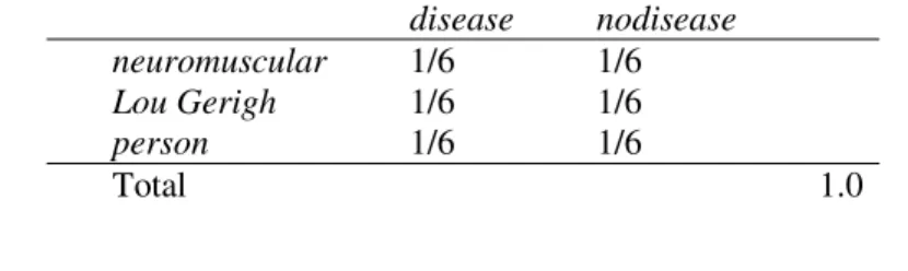
Table 5.2. An example of a distribution that in the most uncertain way satisfies the constraint in Eq. (5.22).

disease nodisease

neuromuscular 1/6 1/6

Lou Gerigh 1/6 1/6

1/6 1/6

Total 1.0

From the training set we learn that in 50% of the examples in which a dis- ease is mentioned the term Lou Gerigh occurs and that 70% of the exam- ples of the training set are classified as disease imposing the following constraints expressed by the feature functions:

3The model is not restricted to binary features. For binary features efficient numerical methods exist for computing the model parameters of Eq. (5.35).

person

(15)

fLouGehrig

ff (x, y)= 1 if x1= Lou Gerigh and y = disease 0 otherwise

®

¯®® (5.24)

fdisease

ff (x, y)= 1 if y= disease 0 otherwise

®

¯®® (5.25)

In this simplified example, our training set does not give any information about the other context terms. The problem is how to find the most uncertain model that satisfies the constraints. In Table 5.3 one can again look for the most uniform distribution satisfying these constraints, but the example makes it clear that the choice is not always obvious. The maximum entropy model offers here a solution. Thus, when training the system, we choose the model p* that preserves as much uncertainty as possible, or which maximizes the entropy H(HH p(( ) between all the models p∈ P that sat- isfy the constraints enforced by the training examples.

H(p(( ) = ⁻

¦

) , (

) , ( log ) , (

y x

y x p y x

p (5.26)

_p_* _arg_max_H₍_p₎

P p∈

= (5.27)

In the examples above we have considered an input training example char- acterized by a certain label y and a feature vector x, containing the context of the word (e.g., as described by surrounding words and their POS tag).

We can collect n number of training examples and summarize the training sample S in terms of its empirical probability distribution: p~ defined by:

(5.24) and (5.25).

disease nodisease

neuromuscular ? ?

Lou Gerigh 0.5 ?

? ?

Total 0.7 1.0

person

Table 5.3. An example of a distribution that satisfies the constraints in Eqs. (5.22),

(16)

˜p(x, y)≡no

n (5.28) where no = number of times a particular pair (x(( ,y) occurs in S andS no ≥^0.

We want to compute the expected value of the feature function fff with re-j

spect to the empirical distribution ˜p(x, y) .⁴

E^˜p E

E ( fff )^j = ˜p(x, y) fff (x, y)j x,y

¦

(5.29) The statistics of a feature function are captured and it is required that the model that we are building accords with it. We do this by constraining the expected value that the model assigns to the corresponding feature func- tion fff . The expected value of fj ff with respect to the model p(y x) is:j

E^p E

E ( fff )^j = ˜p(x) p( y x) fff (x, y)j x,y

¦

(5.30) where ˜p(x) is the empirical distribution of x in the training sample. We constrain this expected value to be the same as the expected value of fffjin the training sample, i.e., the empirical expectation of fff . That is we require:j

) ( )

( ^j ^~^p ^j

p f^j E^~^p^p f^j

E^p^p = (5.31) Combining Eqs. (5.29), (5.30) and (5.31) yields the following constraint equation:

˜p(x) p( y x) fff (x, y)^j

x,y

¦

⁼ ^{˜p(x, y) f}^ff^j^{(x, y)}

x,y

¦

^(5.32)

By restricting attention to these models p(y x) for which Eq. (5.31) holds, we are eliminating from consideration those models that do not agree with the training samples. In addition, according to the principle of maximum entropy we should select the distribution which is most uniform. A

4The notation is sometimes abused: fff (x_j(( ,y) will both denote the value of fff for a _j particular pair (x(( ,y) as well as the entire function fff ._j

(17)

mathematical measure of the uniformity of a conditional distribution p(y x) is provided by the conditional entropy. The conditional entropy H(HH Y X)XX measures how much entropy a random variable Y has remaining, if weY have already learned completely the value of a second random variable X.

The conditional entropy of a discrete random Y givenY X:

H(Y X)= p(x)H(Y X= x)

x∈X

¦

(5.33) H (Y X)= − p( x) p( y x) log p( y x)

y

¦

∈Y

x

¦

∈X ^(5.34)

or⁵

H ( p)≡ − ˜p(x) p( y x)

x∈X ,y∈Y

¦

log p( y x)

Note that ˜p(x) is estimated from the training set and p(y(( x) is the learned x model. When the model has no uncertainty at all, the entropy is zero.

When the values of y are uniformly distributed, the entropy is log y . It has been shown that there is always a unique model p*(y x) with maximum entropy that obeys the constraints set by the training set. Considering the feature vector x of a test example, this distribution has the following expo- nential form:

p * ( y x)=1

Zexp λλλλλ^j^jj^f^{ff (x, y)}^j

j=1 k

¦

^{, 0}^< ^λ^λλ^j ^{< ∞} ^(5.35)

where fffj(x(( , y) is one of the k binary-valued feature functions λ^j

λ= parameter adjusted to model the observed statistics Z = normalizing constant computed as:

Z

Z= exp

(

λλλλλ^j^jj^fff (x, y)^j

)

j=1

¦

k

¦

y )

))

(5.36)

So, the task is to define the parameters λλλjjⁱⁿp which maximize H(HH p(( ). In simple cases we can find the solution analytically, in more complex cases

5Following Berger et al. (1996) we use here the notation H(p(( ) in order to empha- size the dependence of the entropy on the probably distribution p instead of the common notation H (H Y X) where Y and Y X are random variables. X

( )

(18)

we need numerical methods to derive λλλ^j^j given a set of constraints. The problem can be considered as a constrained optimization problem, where we have to find a set of parameters of an exponential model, which maximizes its log likelihood. Different numerical methods can be applied for this task among which are generalized iterative scaling (Darroch and

We also have to efficiently compute the expectation of each feature function. Eq. (5.30) cannot be efficiently computed, because it would in- volve summing over all possible combinations of x and y, a potentially in- finite set. Instead the following approximation is used, which takes into account the n training examples xi:

E^p E

E ( fff )^j =1

n p( y xⁱ) fff (x^j ⁱ, y)

y i=1

¦

n

¦

(5.37) The maximum entropy model has been successfully applied to natural language tasks in which context-sensitive modeling is important (Berger et al., model has been used in named entity recognition (e.g., Chieu and Hwee nition (Fleischman et al., 2003; Mehay et al., 2005). The maximum entropy model offers many advantages. The classifier allows to model dependen- cies between features, which certainly exist in many information extraction tasks. The classifier has the advantage that there is no need for an a priori feature selection, as features that just are randomly associated with a certain class, will keep their randomness in the model. This has the advantage that you can train and experiment with many context features in the model, in an attempt to decrease the ambiguity of the learned patterns. Moreover, the principle of maximum entropy states that when we make inferences based on incomplete information, we should draw them from a probability distribution that has the maximum entropy permitted by the information training set is often incomplete given the large variety of natural language patterns that convey the semantic classes sought. Here, the maximum entropy approach offers a satisfactory solution.

The above classification methods assume that there is no relation between various classes. In information extraction in particular and in text understanding in general, content is often dependent. For instance, when there is no grant approved, there is also no beneficiary of the grant. Or, more formally one can say: There is only one or a finite number of ways in Ratcliff, 1972), improved iterative scaling (Della Pietra et al., 1997), gradient ascent and conjugate gradient (Malouf, 2002).

2002), coreference resolution (e.g., Kehler, 1997) and semantic role recog-

that we do have (Jaynes, 1982). In many information extraction tasks, our 1996; Ratnaparkhi, 1998) among which is information extraction. The

(19)

which information can be sequenced in a text or in a text sentence in order to convey its meaning. The scripts developed by Schank and his school in the 1970s and 1980s are an illustrative example (e.g., you have to get on the bus before you can ride the bus). But also, at the more fine-grained level of the sentence the functional position of an information unit in dependency with the other units defines the fine-grained meaning of the sentence units (e.g., semantic roles). In other words, information contained in text often has a certain dependency, one cannot exist without the other, or it has a high chance to occur with other information. This dependency and the nature of the dependency can be signaled by lexical items (and their co-occurrence in a large corpus) and refined by the syntactical constructs of the language including the discourse structure.

In pattern recognition there are a number of algorithms for context- dependent classification. In these models, the objects are described by feature vectors, but the features and their values stored in different feature vectors together contribute to the classification. In order to reduce the computational complexity of the algorithms the vectors are often processed in a certain order and the dependency upon vectors previously processed is limited. The class to which a feature vector is assigned depends on its own value, on the values of the other feature vectors and on the existing relation among the various classes. In other words, having obtained the class cifor a feature vector xi, the next feature vector could not always belong to any other class. In the following sections we will discuss two common approaches to context-dependent information recognition: Hidden Markov models and conditional random fields. We foresee that many other useful context dependent classification algorithms will be developed in text understanding. In context-dependent classification, feature vectors are often referred to as observations. For instance, the feature vector xi occurs in a sequence of observations X = (X ((x1,…, xTTT).

5.4 Hidden Markov Models

In Chap. 2 we have seen that finite state automata quite successfully rec- ognize a sequence of information units in a sentence or a text. In such a model a text is considered as a sequence of symbols and not as an unor- dered set. The task is to assign a class sequence Y= (y(( 1,…,yTTT) to the se- quence of observations X = (X ((x1,…, xTTT). Research in information extraction has recently investigated probabilistic sequence models, where the task is to assign the most probable sequence of classes to the chain of observa- tions. Typically, the model of the content is implemented as a Markov 5.4 Hidden Markov Models 107

(20)

chain of states, in which transition probabilities between states and the probabilities of emissions of certain symbols of the alphabet are modeled.

The states are shown as circles and the start state is indicated as start.

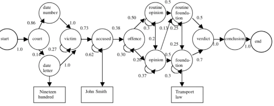
Possible transitions are shown by edges that connect states, and an edge is labeled with the probability of this transition. Transitions with zero probability are omitted from the graph. Note that the probabilities of the edges that go out from each state sum to 1. From this representation, it should be clear that a Markov model can be thought as a (non-deterministic) finite state automaton with probabilities attached to each edge.

Fig. 5.3. An example Markov model that represents a Belgian criminal court decision. Some examples of emissions are shown without their probabilities.

court

start victim accused

date numbe r

date letter

offence routine opinion

opinion routine founda- tion

founda- tion

verdict

Nineteen hundredd

John Smith Transport

law 1.0

0.86

0.144

1.0

1.0 0.27

0.73

0.62 0.38

0.30 0.50

0.200

0.37 0.3

0.7 0.25 0.25 0.2 0.3

0.5

1.0 1 0.133

0.5 0

conclusion end 1.0

as a Markov chain.

In Fig. 5.3 the content of a Belgian criminal court decision is modeled

The probability of a sequence of states or classes Y = (Y y1,…,yTTT) is easily calculated for a Markov chain:

P(y1,…,yTT) = P(y1)P(y2y1) P(y3y1, y2) … P (yT y1,…,yT-1) (5.38) A first order Markov model assumes that class dependence is limited only within two successive classes yielding:

P(y1,…,yTT) =P(y1)P(y2y1) P(y3y2)…P (yT yT-1) (5.39)

(21)

109

= P(y) P( yⁱyⁱ− 1)

i= 2

∏

T (5.40) In Fig. 5.3 only some of the emission symbols are shown. The models that we consider in the context of information extraction have a discrete output, i.e., an observation outputs discrete values.

A first order Markov model is composed of a set of states Y with speci-Y fied initial and final states y1and yTTT, a set of transitions between states, and a discrete vocabulary of output symbols¦¦ = {σσ¹^,σσσ²^,…,σσσ^k}. In information extraction the emission symbols are usually words. The model generates an observation X = (X ((x1,…,xTTT) by beginning in the initial state, transitioning to a new state, emitting an output symbol, transitioning to another state, emitting another symbol, and so on, until a transition is made into the final state. The parameters of the model are the transition probabilities P(yiyi-1) that one state follows another and the emission probabilities P(x(( iyi) that a state emits a particular output symbol.⁶

Classification regards the recognition of the most probable path in the model. For the task of information extraction this translates into the following procedure. Having observed the following sequence of feature vec- tors X = (x(( 1,…,xTTT), we have to find the respective sequence of classes or states Y = (Y y1,…,yTTT) that is most probably followed in the model. We com- pute Y* for which

Y*= argmax

Y

P(Y X) (5.41)

P(Y X)=P(y¹)P(x¹y¹) P( yⁱyⁱ− 1)P(xⁱ

i= 2

∏

T ^yⁱ⁾ ^(5.42)

In order to compute the most probable path the Viterbi algorithm is used.

Instead of a brute-force computation, by which all possible paths are computed, the Viterbi algorithm efficiently computes a subset of these paths. It is based on the observation that, if you look at the best path that goes through a given state yiat a given time ti, the path is the concatenation of the best path that goes from state y1 to yi(while emitting symbols corre- sponding to the feature vectors x1to xirespectively at times t1to ti) with the best path from state yi to the final state yT(while emitting symbols corre- sponding to the feature vectors xi + 1 to xTrespectively at times ti+1to tTTT).

This is because the probability of a path going through state yi is simply the product of the probabilities of the two parts (before and after yi), so that

6We mean here the discrete symbol that is represented by the feature vector x.

5.4 Hidden Markov Models

(22)

the maximum probability of the global path is obtained when each part has a maximum probability.

When we want to train a Markov model based on labeled sequences XXXall

there are usually two steps. First, one has to define the model of states or classes, which is called the topology of the model. Secondly, one has to learn the emission and transition probabilities of the model. The first step is usually drafted by hand when training an information extraction system (although at the end of this section we will mention some attempts to learn a state model). In the second step, the probabilities of the model are learned based on the classified training examples. The task is learning the probabilities of the initial state, the state transitions and the emissions of a modelµ^.

In a visible Markov model (Fig. 5.4), the state sequence that actuallyl generated an example is known, i.e., we can directly observe the states and the emitted symbols. If we can identify the path that was taken inside the model to produce each training sequence, we are able to estimate the probabilities by the relative frequency of each transition from each state and of emitting each symbol. The labeling is used to directly compute the probabilities of the parameters of the Markov model by means of maximum likelihood estimates in the training set XXX . The transition probabilities all

P(y’ y) and the emission probabilities P(x(( y) are based on the counts of respectively the class transitionsξξξ⁽y->y’) orξξξ⁽y,y’) and of the emissions oc- curring in a classγ(y) where y↑x↑↑ i considered at the different times t:

P(y' y)= ξ^t ξξ^{(y, y )}

t=1 T−1

¦

γ^t γ ^(y)

t=1 T−1

¦

(5.43)

P(x y)=

γ^t γ ^(y)

t=1 and y↑x T

¦

γ^t γ ^(y)

t=1 T

¦

(5.44)

state sequence that the model passed through when generating the training examples. The states of the training examples are not fully observable.

This is often the case in an information extraction task from a sequence of

’

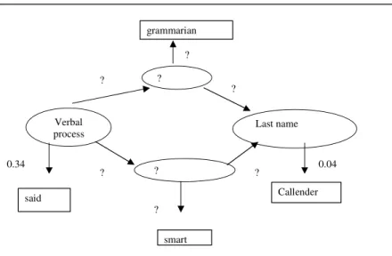
In a hidden Markov modell (Rabiner, 1989) (Fig. 5.5) you do not know the

(23)

111

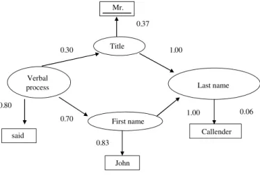
words. Each state (e.g., word) is associated with a class that we want to extract. Some states are just background states, when they represent information not to be extracted or semantically labeled. As a result some of the words are observed as emission symbols and have an unknown class or state.

In this case the transition and emission probabilities are inferred from a sequence of observations via some optimization function that is iteratively computed. The training of parameters is usually performed via the Baum- Welch algorithm, which is a special case of the Expectation-Maximization

Fig. 5.4. Example of a visible Markov Model for a named entity recognition task.

and the emissions of the modelµµ. The Baum-Welch approach is character- ized by the following steps:

1. Start with initial estimates for the probabilities chosen randomly or according to some prior knowledge.

2. Apply the model on the training data:

Expectation step (E): Use the current model and observations to calculate the expected number of traversals across each arc and the expected number of traversals across each arc while producing a given output.

5.4 Hidden Markov Models

Title

First name Verbal

process Last name

said

John

Callender Mr.

0.30

0.70

1.00

1.00 0.80

0.37

0.06

0.83

The task is learning the probabilities of the initial state, the state transitions algorithm (EM) (Dempster et al., 1977).

into a model that most likely produces these ratios.

Maximization step (M): Use these calculations to update the model

(24)

Fig. 5.5. Example of a hidden Markov model for a named entity recognition task.

3. Iterate step 2 until a convergence criterion is satisfied (e.g., when the differences of the values with the values of a previous step are smaller than a threshold valueεεε^).

Expectation step (E)

We consider the number of times that a path passes through state y at time t and through state

t y’ at the next time t + 1 and the number of times thist state transition occurs while generating the training sequences XXXalll given the parameters of the current modelµµ. We then can define:

ξ^t

ξξ^(y,y’) ≡ ξξξ^t^{(y,y’ X}^X^{X ,}^all µµµ^{) =}ξξξ^t^{(y, y , X}^X^X^allµµµ⁾

P(XXX^allµµµ⁾ ^(5.45)

=αα⁽^y^t= y)P(y y)P(x^t^{+ 1}y )ββ⁽^y^t^{+ 1}= y )

P( XXX^allµµ⁾ ^(5.46)

whereα(y^t= y) represents the path history terminating at time t and statet y (i.e., the probability of being at state y at time t and outputting the first t symbols) and ββ⁽^y^t^{+ 1}= y )represents the future of the path, which at time t + 1 is at state y’ and then evolves unconstrained until the end (i.e., the

?

? Verbal

process Last name

smart

Callender grammarian

?

0.34 0.04

’

(25)

113

probability of being at the remaining states and outputting the remaining symbols). We define also the probability of being at time t at statet y:

γ^t

γγ ^(y)≡γγγ^t^{(y X}^X^{X ,}^allµµµ⁾=α^(y^t= y)β^(y^t= y)

P(XXX^allµµµ⁾ (5.47) γ^t^{( y)}

t=1 T−1

¦

can be regarded as the expected number of transitions from state y given the model µµand the observation sequences^XXX .all

¦

⁻

= 1

1

) , (

T

t

t y y

ξ can be regarded as the expected number of transitions from state y to state y’, given the modelµand the observation sequences XXX .all

Maximization step (M)

During the M-step the following formulas compute reasonable estimates of the unknown model parameters:

¦

−

=

−

= = 1

1 1

1

) (

) , ( )

( _T

t t T

t t

y y y y

y P

γ ξ

(5.48)

P(x y)=

γ^t γγ^(y)

t=1 and y↑x T

¦

γ^t γγ^(y)

t=1 T

¦

(5.49)

P ( y)=γ¹^{( y)} (5.50) Practical implementations of the HMM have to cope with problems of zero probabilities as the values of α^(yt) and ββ⁽⁽⁽^yt) are smaller than one and when used in products tend to go to zero, which demands for an appropriate scaling of these values.

A hidden Markov model is a popular technique to detect and classify a 5.4 Hidden Markov Models

’

linear sequence of information in text. The first information extraction

’