國立臺灣大學工學院化學工程學研究所 碩士論文
Graduate Institute of Chemical Engineering College of Engineering
National Taiwan University Master Thesis
COSMO-SAC 模型氫鍵描述之修正 及其在離子液體之應用
Modification of Hydrogen Bonding Interactions for COSMO-SAC Model and Its Applications in Ionic Liquids
張峻愷 Chun-Kai Chang
指導教授: 林祥泰 博士
Advisor: Shiang-Tai Lin, Ph.D.
致謝
時光飛逝,不知不覺也在COMET 待了四年,從當時的什麼都不會的菜鳥到看似可
以cosplay 碩士的玩家,當然要感謝從大三時就收留我的林祥泰老師,從老師身上
不僅學到做研究的技巧,更重要的是做研究的態度。吳台偉老師也在研究上給予了 許多獨到的見解刺激,讓我在研究上有所突破,度過最困難的時光,往後便頭過身 就過。印度理工學院(IIT)的 S.R Gadre 教授也給了幾個 MESP 找孤電子對的範例,
也幫助我在研究上面有更大的信心,知道這是一個可行的方向。此外,也感謝謝介 銘老師願意擔任這次的口試委員,在口試的討論中,也讓我更認識自己的研究,產
生很多新的想法可以提供給未來的學弟學妹來讓COSMO-SAC 模型更臻完美。威
霖和立行兩位大學長則是在寫程式上面給予我很大的啟發,讓我掌握了做模擬的
基本工具。再來是智為學長所教導的COSMO-SAC 模型之基本概念和操作,則是
使我獲得了在 COMET 的寶劍,也讓我可以開始在研究上做出一些不足掛齒的貢
獻。在研究主題上,Lee 在離子液體的領域也給予我些許指導,使我能更快上手。
也感謝實驗室現役成員:子芳、軒豪、Aditya、昌哲、德謙、Dalip、興豪、力行、
垚煌、政廷、晨軒、柏偉、曉丰、姿妤、藍天、浩恩、奕安,有你們在實驗室聊天、
聊研究,也讓研究生生涯就沒那麼苦悶了。COMET 待了幾年,除了科研的進步,
更多的是培養做研究的耐心並且能夠更加耐得住寂寞,也學會怎麼跟自己相處。
感謝我的家人(還有家人候選)不論是精神上經濟上一直支持我,也感謝神讓我遇到 不管是對我友善或是有敵意的人,有這些人出現在我生命中,才造就了現在的我。
中文摘要
本作共分為兩部分,第一部份修正COSMO-SAC 活性係數模型的氫鍵作用力描述。
近期(2017)有文獻指出,如將氫鍵的方向性考慮至 COSMO-SAC 模型當中,則在耦 合系統之熱力學性質的預測上會有顯著的進步。將氫鍵方向性納入考量的方法之 一 為透 過 價 殼層 電子 對互斥 理論(Valence Shell Electron Pair Repulsion Theory, VSEPR),推測孤電子對(Lone pair, LP)的位置,進而得到孤電子對與質子形成氫鍵 的方向。然而,這種基於分子構型以推得孤電子對的方法在一些分子上會有所侷限,
例如:氫氟酸(HF)以及二甲基亞碸(DMSO)。在這兩個分子中,即無法透過其分子 內部的鍵結關係得到孤電子對之位置。為了將氫鍵的方向性有效地引入至所有種 類之系統,本論文利用分子電位分布(Molecular Electrostatic Potential Map, MESP) 尋找分子局部電位的低點,並將該局部低點視為孤電子對的位置。以此方法決定氫 鍵的方向後,除了不須再依靠分子結構取得氫鍵的方向之外,所有中性分子系統在 無限稀釋下的活性係數、汽液相平衡、液液相平衡、辛醇-水分配係數等熱力學性 質的預測上亦有所進步(中性分子之汽液相平衡預測準確度取得約 5-7%之進步)。
本作第二部份則將第一部分所提及的新方法用在離子液體系統中,並且搭配新提 出之符合熱力學一致關係式模型,也在稀薄離子液體的系統中取得了顯著的進步 (滲透係數之預測準確度改善約 10%),成功將氫鍵作用力的方向性更廣泛的應用至 離子液體等帶電系統中。
關鍵字: 感應電荷、COSMO-SAC、COSMO-SAC (DHB)、分子電位分布、氫鍵、
Abstract
A new approach for determining directional hydrogen bonding interactions in the COSMO-SAC model is proposed for both neutral and charged species. In a recent work, Chen and Lin showed that the consideration of directional hydrogen bonding in the COSMO-SAC model significantly improves the description of solvation properties of associating fluids. In their method, the direction of a hydrogen bond was determined based on the VSEPR theory; however, this geometric approach does not reflect the local electronic environment of the lone pairs and cannot be applied to certain molecules such as DMSO and HF. In this work, we adopt a new scheme that determines the hydrogen bond acceptors of a molecule based on the minima in the molecular electrostatic potential (MESP). The hydrogen bonding directions thus determined result in improvements (about 5-7% for VLE) in the prediction of the COSMO-SAC model for a variety of thermodynamic properties and phase equilibria of neutral species, such as vapor-liquid equilibrium (VLE), liquid-liquid equilibrium (LLE), infinite dilution activity coefficient (IDAC), octanol-water partition coefficient (Kow). We also apply this new approach on charged species, such as ionic liquids (ILs), and apply with a new proposed extended PDH model. The improvement on IL-diluted region (about 10% for osmotic coefficient) is also reported.
Keywords: Screening charge, COSMO-SAC, COSMO-SAC (DHB), molecular electrostatic potential, hydrogen bond, ionic liquid, activity coefficient, phase behavior, partition coefficient, osmotic coefficient
Table of Contents
致謝 ... i
中文摘要 ... ii
Abstract ... iii
Table of Contents ... iv
List of Figures ... vii
List of Tables ... xii
Chapter 1. Introduction ... 1
1.1 The Perspectives of Liquid Models in Chemical Engineering ... 1
1.2 The Challenge and Evolution of the Description of Hydrogen Bonding Interactions in the COSMO-SAC Model ... 3
1.3 An Extension – From Neutral Species to Ionic Liquids ... 5
Chapter 2. Theory ... 7
2.1 The COSMO-SAC Model ... 7
2.2 Treatments on HB Interactions ... 9
2.3 The Pitzer-Debye-Hückel Model ... 17
2.4 A Thermodynamically Consistent Extended PDH Model for Ionic Liquid Systems ... 18
2.5 Partial Dissociation of Ions with Consideration of Chemical Reaction ... 22
Chapter 3. Computational Details ... 23
3.1 Information of Quantum Chemical Calculations... 23
4.1 Comparison of Thermodynamic Properties from COSMO-SAC (DHB) Using
MESP versus VSEPR ... 28
4.2 Comparison of Hydrogen Bond Surfaces in the COMSO-SAC (DHB)/VSEPR and COSMO-SAC (DHB)/MESP ... 37
4.3 Summary ... 43
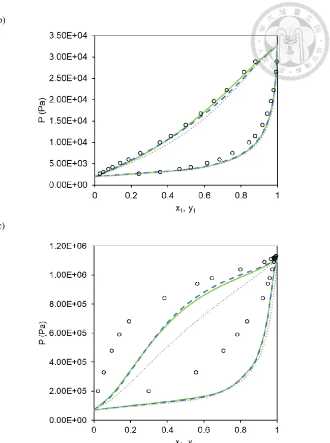
Chapter 5. Improved Prediction of Phase Behaviors of Ionic Liquids with Consideration of Directional Hydrogen Bonding Interactions ... 44
5.1 IDAC of a Neutral Solvent in ILs ... 44
5.2 Osmotic Coefficient of Neutral Solvent-ILs Binary Mixtures ... 46
5.3 LLE of Neutral Solvent-ILs Binary Mixtures ... 48
5.4 Degree of Dissociation of Partially Dissociated ILs ... 51
5.5 VLE of Neutral Solvent-ILs Binary Mixtures ... 53
5.6 Summary ... 57
Chapter 6. Conclusion and Future Prospects ... 64
Appendix A. Undetermined Lone Pair Positions by VSEPR ... 67
A.1 Three Types Undermined Lone Pair Positions by VSEPR ... 67
A.2 Lone Pairs for Halothanes Determined by VSEPR ... 68
Appendix B. Examination Thermodynamic Consistency by Chemical Potential from Gibbs Free Energy of Mixing ... 69
B.1 Chemical Potential from Gibbs Free Energy of Mixing ... 69
B.2 Thermodynamic Inconsistency of the Original PDH Model Using Averaged Solvent Properties from All Species ... 72
Appendix C. Comparison of Original PDH Model, PDH Model with Averaged Solvent Properties, and Extended PDH Model ... 74
C.2 Derivation of Thermodynamically Consistent Extended PDH Model ... 76
C.3 Thermodynamic Properties from Different Treatments on Solvent Properties in the PDH Model ... 77
Appendix D. Details of Activity Coefficients Calculations from the Extended Pitzer-Debye-Hückel Model ... 89
D.1 Determination of Molecular Weights, Densities, and Radii for ILs ... 89
D.2 Examples of Activity Coefficients Calculations from the Extended Pitzer- Debye-Hückel Model ... 96
Appendix E. Detail results for Thermodynamic Properties of Demonstrated Examples of Neutral Solvent-IL Binary Systems ... 98
E.1 Details for IDAC and Osmotic Coefficients Results ... 98
E.2 Details for LLE and VLE Results ... 102
Reference ... 109
List of Figures
Figure 1.1-1 Three ways to obtain phase diagrams for chemical engineers ... 2 Figure 1.3-1 Characteristic and application fields of ionic liquids. ... 6 Figure 2.2-1 The hydrogen bond centers (yellow balls) found in VSEPR for water (b) The spatial distribution of COSMO charge density and (c) the HB surface regions of water from COSMO-SAC (DHB)/VSEPR. ... 12 Figure 2.2-2 (a) The hydrogen bond centers found by VSEPR and MESP for water. The green balls stand for the hydrogen bond centers from MESP while the yellow balls stand for that in VSEPR. (b) The HB surface region of water from COSMO-SAC (DHB)/VSEPR. (c) The HB surface region within RcutHB water from COSMO- SAC (DHB)/MESP. Note that the hydrogen bond centers for proton donors are unchanged since the only difference between the two methods is in the treatment of proton acceptors. ... 14 Figure 2.2-3 The hydrogen bond centers determined from MESP for (a) HF, (b) DMSO and (c) methylisocyanate. The green balls stand for the hydrogen bond centers and the black ones stand for electrostatic potential local minima found by MESP. The VSEPR fails to provide the lone pair direction for these compounds. ... 15 Figure 2.2-4 σ-profile of water (a) non hydrogen-bonding level (b) hydrogen-bonding level for each COSMO-SAC model ... 16 Figure 3.3-1 Combination of σ-profiles of cation and anion for ion pairs ... 27 Figure 4.1-1 Comparison of predicted phase diagrams of example VLE binary systems:
(a) ethanol (1) – water (2) at 348.15K (b) 2-methyl-1-propanol (1) – DMSO (2) at 353.15K (c) difluoro methane (1) – hydrogen fluoride (2) at 283.15K. The black
(2) binary systems. The black circles are experimental data [76]. ... 33 Figure 4.1-3 The relationship between predicted and experimental data [76] for the infinite dilution activity coefficient from COSMO-SAC (DHB) (square: MESP circle: VSEPR) ... 35 Figure 4.1-4 The relationship between predicted and experimental data [77] for the octanol-water partition coefficient from COSMO-SAC (DHB) (square: MESP circle:
VSEPR). ... 36 Figure 4.2-1 Comparison of the fraction of hydrogen bonding surface from MESP and VSEPR. ... 41 Figure 4.2-2 Comparison of the effective HB surface charge density: (a) acceptor (b) donor ... 42 Figure 5.1-1 Comparison of IDAC of neutral species in ILs predicted by COSMO-SAC models with α = 0 . (COSMO-SAC 2010: blue circles ; COSMO-SAC (DHB)/MESP: green crosses ) ... 45 Figure 5.2-1 Comparison of osmotic coefficient of (a) 1-propanol-[C1MPy][MeSO4] at 323.15K [80] and (b) water-[C6MIM][Cl] binary system at 313.15K [81] predicted by COSMO-SAC models with α = 1. (COSMO-SAC 2010 : blue chain lines ; COSMO-SAC (DHB)/MESP: green solid lines ; experimental data: black circles ) ... 47 Figure 5.3-1 LLE of (a) water mixed with [C4MIM][PF6] system [82] with α = 0 (b) 1-
butanol mixed with [C4MIM][TF2N] [83] (from different COSMO-SAC models with α0=0.35 (COSMO-SAC 2010: blue chain lines ; COSMO-SAC
COSMO-SAC (DHB)/MESP: green solid lines ; experimental data: black squares ) ... 52 Figure 5.5-1 Comparison of vapor pressure of methanol in [C4MIM][BF4] at 283.15K [85]
(a) ; methanol in [C1MIM][DC1Ph] at 353.15K [86] (b); water in [C8MIM][PF6] at 298.15K [87] (c) from the COSMO-SAC models and experimental data. (α = 0) (COSMO-SAC 2010: blue chain lines ; COSMO-SAC (DHB)/MESP: green solid lines ; experimental data: black circles ) ... 56 Figure A.1-1 Some examples that failed to assign lone pairs positions by VSEPR: (a) HF (b) DMSO and (c) methylisocyanate. Red line segments stand for the auxiliary bond directions while the dotted lines stand for all possible positions of lone pairs. ... 68 Figure A.2-1 Assigning lone pairs in (a) Methyl fluoride and (b) Vinyl fluoride. Red line segments stand for the auxiliary bond directions while the dotted lines stand for all possible positions of lone pairs. ... 68 Figure B.1-1 The of LLE composition determined from (a) co-tangent line in Δμmix −
𝑥𝑠 diagram and (b) equality of activity of each species in each phase for 1-butanol and [C4MIM][BF4] binary mixture at 320K. (gray dotted lines indicates the LLE compositions) ... 71 Figure B.2-1 Long-range contribution of activity coefficient of 1-butanol-[C4MIM][BF4] system at 320K using (a) M2 (b) M3. (solid blue line : solvent; green dashed line : ions; red chain line : GD value) ... 73 Figure C.3-1 VLE and activity coefficient of (a)(b) water-[C1MIM][DC1Ph] at 353.15K [86] and (c)(d) 1-hexene-[C4MIM][PF6] at 283.15K [91] with different treatments of solvent properties in the PDH model. (circles : experimental data; blue lines : overall contribution; orange lines : PDH contribution; solid lines
Figure C.3-2 The change of Aϕ (a), ρ (b) and 1/ϵ𝑠 (c) with mole fraction of neutral solvent in water-[C1MIM][DC1Ph] at 353.1K [86] (dashed line ) and 1- hexene-[C4MIM][PF6] at 283.15K [91] (solid line ) ... 84 Figure C.3-3 Comparison of LLE of (a) 1-pentanol-[C8MIM][BF4] [88] (b) 1-butanol-
[C6MIM][PF6] [89] binary mixtures from different treatments of solvent properties in the PDH model. (circles : experimental data; solid lines : M3; dashed lines : M2; chain lines : M1) ... 85 Figure C.3-4 Comparison of IDAC of neutral species in ILs from different treatments of solvent properties in the PDH model. (gray diamonds : M1 ; green crosses : M2 ; blue circles : M3) ... 86 Figure C.3-5 Osmotic coefficient (a) and activity coefficient (b) of 1-propenol-
[C1MPy][MeSO4] at 323.15K [90] from different treatments of solvent properties in the PDH model. (circles : experimental data; blue lines : overall contribution; orange lines : PDH contribution; solid lines : M3; dashed lines : M2; chain lines : M1) ... 87 Figure E.1-1 Comparison of IDAC of neutral species in ILs predicted by COSMO-SAC models with (a) α = 1 and (b) α0 = 0.35. (COSMO-SAC 2010: blue circles ; COSMO-SAC (DHB)/MESP: green crosses ) ... 99 Figure E.1-2 Comparison of osmotic coefficient of 1-propanol-[C1MPy][MeSO4] at 323.15K [80]: (a) α = 0 (b) α0 = 0.35 and water-[C6MIM][Cl] binary system at 313.15K [81]: (c) α = 0 (d) α0 = 0.35 predicted by COSMO-SAC models.
(COSMO-SAC 2010: blue chain lines ; COSMO-SAC (DHB)/MESP: green
COSMO-SAC models (COSMO-SAC 2010: blue chain lines ; COSMO-SAC (DHB)/MESP: green solid lines ; experimental data: black circles ) ... 104 Figure E.2-2 Comparison of vapor pressure of methanol in [C4MIM][BF4] at 283.15K [85] with α = 1 (a) and α0 = 0.35 (b); methanol in [C1MIM][DC1Ph] at 353.15K [86] with α = 1 (c) and α0 = 0.35 (d); water in [C8MIM][PF6] at 298.15K [87]
with α = 1 (e) and α0 = 0.35 (f) from the COSMO-SAC models and experimental data. (COSMO-SAC 2010: blue chain lines ; COSMO-SAC (DHB)/MESP: green solid lines ; experimental data: black circles ) . 108
List of Tables
Table 2.4-1 Expressions of η and τ for different treatments of solvent properties in the generalized PDH model ... 21 Table 3.1-1 Parameters in different COSMO-SAC models considered in this work. .... 25 Table 3.2-1 The three schemes discussed in this work. ... 26 Table 4.1-1 Prediction accuracy of COSMO-SAC models for VLE, LLE, IDAC and Kow
... 29 Table 4.1-2 RMS error of IDAC by VSEPR and MESP methods for different systems 34 Table 4.2-1 Some typical examples for comparison of HB segments determined by COSMO-SAC (DHB)/VSEPR and COSMO-SAC (DHB)/MESP ... 39 Table 5.6-1 Comparison of performance in prediction different thermodynamic properties and phase equilibria based on three treatments of the solvent properties ... 58 Table 5.6-2 Some examples of hbc, HB surfaces, and σ -profiles in HB-level of the molecules discussed in this work determined by the COSMO-SAC 2010 and the COSMO-SAC (DHB)/MESP. (black balls: hbc) ... 59 Table C.1-1 Treatments of Solvent Properties in the PDH Model ... 75 Table C.3-1 Comparison of performance in prediction different thermodynamic properties and phase equilibria based on three treatments of the solvent properties in the PDH model ... 88 Table D.1-1 Summary of cations and anions of ionic liquids considered in this work .. 90 Table D.2-1 Parameters and results of 1-pentanol/[C8MIM][BF4] and 1-
Chapter 1. Introduction
1.1 The Perspectives of Liquid Models in Chemical Engineering
Liquid model plays an important role in chemical engineering process, especially in the part of separation. To be more specific, chemical engineers rely on phase diagrams to design proper separation processes such as distillation, absorption of gases, adsorption isotherms, liquid-liquid extraction, crystallization, and leaching because phase diagrams provide the needed thermodynamic information such as compositions at vapor-liquid equilibrium (VLE), liquid-liquid equilibrium (LLE), and solid-liquid equilibrium (SLE).
Besides the composition at equilibrium, thermodynamic properties such as infinite dilution activity coefficient (IDAC), octanol-water partition coefficients (Kow), and osmotic coefficients ( 𝜙 ) are also useful indexes while developing and optimizing chemical processes. As a result, it is reasonable to claim that phase diagrams are indispensable to process developments.
There are several ways to obtain phase diagrams. They all help us better understand the phase behaviors of a mixture. First, it is impossible to refuse the bright side that experiments provide the truth of the behaviors of systems of interest while they are sometimes time-consuming to wait the system to be equilibrium. The cost of time and money sometimes is not affordable for engineers to explore the properties of systems of interest. To compensate the dark side of experiments, thermodynamic modeling comes in.
There are basically two kinds of modeling type: correlative models and theoretically- based models. Correlative models such as UNIQUAC [1] and NRTL [2] are correlated
Consequently, they are accurate when interpolate the experimental data. Still, the drawback of the correlative models is no more under the table when there are lacking the species-dependent parameters of the interested systems.
Figure 1.1-1 Three ways to obtain phase diagrams for chemical engineers
Contrarily, theoretical models use a set of universal parameters to predict the phase behaviors for systems of interest. The COSMO-based activity coefficient models, such as COSMO-RS[3] and COSMO-SAC [4], are powerful methods for predicting phase equilibria involving liquid mixtures [5-7]. In these methods, the interactions between molecules in the liquid state are determined based on the apparent screening charges induced at the molecular surface when considering the molecule as embedded in a perfect conductor [8]. Since such information can be obtained from quantum mechanical
1.2 The Challenge and Evolution of the Description of Hydrogen Bonding Interactions in the COSMO-SAC Model
It has been noted [27, 28] that the prediction accuracy from theoretically-based method is often reduced for mixtures containing associating fluids. Therefore, there has been a continuous effort toward improving the description of hydrogen bonding interactions.[12, 27, 29]
In the original COSMO-based models, the hydrogen bonds were assumed to form only between highly polarized surfaces, and the strength of the interactions was empirically assumed to be proportional to the surface charge density of the hydrogen bonding donor- acceptor pairs. Given the experimental observations that the strength of a hydrogen bond depends on the identity of the donor-acceptor pair, Hsieh et al. [27] proposed to estimate the interaction strength based on the identity of the hydrogen bonding surface (O, N, or F) in addition to the screening charge densities. Such an approach indeed improves the description of associating fluids, however, at the cost of introducing additional empirical parameters. More recently, Chen and Lin [12] proposed a new perspective in describing the hydrogen bonding interactions by recognizing the relative orientations of the donor and the acceptor. Specifically, a hydrogen bond is formed between a donor-acceptor pair along the direction of the electron lone pair, determined based on the Valence Shell Electron Pair Repulsion (VSEPR) theory [30]. Using this approach, Chen and Lin reported a remarkable improvement in describing the solvation properties of ions and the phase equilibria of associating fluids. Despite their success, the geometric VSEPR method of determining the spatial direction of a hydrogen bond is not applicable for three types molecules: most of molecules that contain F (e.g. hydrogen fluoride and vinyl fluoride),
table (e.g. sulfones and phosphine oxides) and O appearing in the terminal of linear functional groups (e.g. ketenes and cyanates). This is because the method proposed by Chen and Lin utilizes the bond directions for determining the lone pairs directions of the acceptor atom. The location of lone pairs cannot be unambiguously defined in these three types of molecules. Furthermore, VSEPR does not explicitly account for the possible change in directions of lone pairs as a result of changes in local environment due to the presence of strongly electronegative or electropositive atoms. The difficulty of arranging desired positions of lone pairs and lone pairs that may be arranged in molecules that contain F by VSEPR are illustrated in Appendix A.
In additional to the geometric VSEPR approach, it has been proposed that the direction of a lone pair can be determined by physical observables, such as the molecular electron density (MED) [31-33] and molecular electrostatic potential (MESP) [34-40]. Using the MESP, for example, the lone pair position is determined from the local minimum of the molecular electrostatic potential of the given molecule. In this work, we adopt the MESP approach for identifying the directions of lone pairs and hydrogen bonding surfaces in the COSMO-SAC (DHB) model. We show that this new approach provides a robust and slightly more accurate description of solvation and thermodynamic properties, including VLE, LLE, IDAC and Kow. More importantly, this method is generally applicable for all types of compounds as the needed electrostatic potential can be obtained from quantum chemical calculations.
1.3 An Extension – From Neutral Species to Ionic Liquids
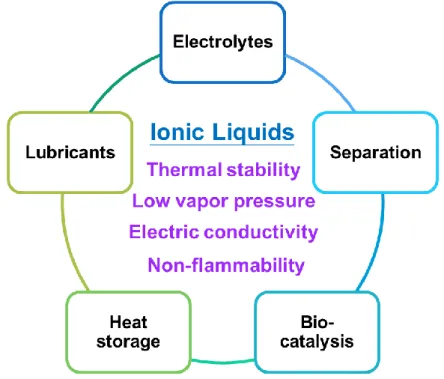
ILs have become the focus of attention for designing new environmental friendly solvents these decades due to their unique properties such as high thermal, chemical stability, and ion conductivity [41]. People are able to take the advantage of their high ion conductivity to design electrochemical devices such as batteries [42]. More importantly, low melting point of ILs indicates that people can treat ILs as liquid solvent at ambient temperature, which is a less energy-consuming choice of working fluid for chemical processes [43].
For example, ILs have been reaction media for biopolymer fiber formation [44], extraction solvent for removal of sulfur compounds [45], entrainer for separation of azeotropic mixtures [46], combination working fluid with supercritical carbon dioxide [47].
Because of the wide range usage of ILs in industry [48], it is important to understand their thermodynamic properties and phase behaviors. Therefore, many experimental measurements [49-51] have been conducted and models developed for predictions.
Liquid models such as UNIQUAC [1], UNIFAC [52], and NRTL [2] model are commonly correlated from experimental phase equilibria data and they are able to give a robust and accurate prediction for interpolation. COSMO based models such as COSMO-RS [3] and COSMO-SAC [4] are based on quantum chemical calculations and thus can give people a predictive way to extrapolate and to explore phase behaviors of fluids that without reported experimental data. Using COSMO-SAC 2010 [27], Lee and Lin [53, 54] also took chemical reaction into consideration to model the behavior of ILs and also reported reasonable results that captured experimental data.
With the success in improving directional hydrogen bonding interactions in neutral species, we adopt the MESP approach for identifying the directions of lone pairs and hydrogen bonding surfaces in the COSMO-SAC (DHB) model [55] to modeling ILs. In Chapter 5, we show that this new approach provides a robust and slightly more accurate description of solvation and thermodynamic properties of ILs systems, including VLE, LLE, IDAC and osmotic coefficients. To repeat, this method is applicable for all types of compounds, from neutral species to charged species, as the needed electrostatic potential can be obtained from quantum chemical calculations.
Figure 1.3-1 Characteristic and application fields of ionic liquids.
Chapter 2. Theory
2.1 The COSMO-SAC Model
The activity coefficient of a chemical species in a mixture can be determined from the difference in solvation free energy of the species in the mixture and in its neat liquid [56]
as
lnγ𝑖/𝑠̅ = Δ𝐺𝑖/𝑠̅
∗𝑠𝑜𝑙−Δ𝐺𝑖/𝑖∗𝑠𝑜𝑙
𝑅𝑇 + ln𝐶𝑠̅
𝐶𝑖 (2.1-1)
where 𝑐𝑖 and 𝑐𝑠̅ stand for the molar concentration of species i in a pure fluid and in a solution, respectively. R is the gas constant and T is the temperature. The solvation free energy, Δ𝐺𝑖/𝑗∗𝑠𝑜𝑙, is the work required to transfer a solute molecule i from a point in the ideal gas phase to another point in solution j under constant temperature and pressure.
Using a perfect conductor as a reference solvent, the solvation free energy can be calculated as the sum of contributions from three different terms accounting for cavity formation (cav), ideal solvation (is) and restoring energy (res),
ΔGi/𝑠̅∗sol= ΔGi/𝑠̅∗cav+ ΔGi/𝑠̅∗is+ ΔGi/𝑠̅∗res (2.1-2) where ΔGi/𝑠̅∗cav is the Gibbs free energy of cavity formation, ΔGi/𝑠̅∗is is the ideal solvation energy and ΔGi/𝑠̅∗res is the restoring energy. Lin and Sandler [4] showed that the difference in the cavity formation energy for a solute being in the solvent and its pure state can be obtained from the Staverman-Guggenheim model [57] as
Δ𝐺𝑖/𝑠̅∗𝑐𝑎𝑣−Δ𝐺𝑖/𝑖∗𝑐𝑎𝑣
𝑅𝑇 = lnγi/𝑠̅𝑆𝐺 −ln𝐶𝑠̅
𝐶𝑖 (2.1-3)
where the lnγi/s𝑆𝐺 term takes into consideration the molecular size and shape difference between both solute and solvent
ln𝛾𝑖/𝑠̅𝑆𝐺 = ln𝜙𝑖
𝑥𝑖 +𝜁
2𝑞𝑖ln𝜃𝑖
𝜙𝑖+ 𝑙𝑖 −𝜙𝑖
𝑥𝑖𝛴𝑗𝑥𝑗𝑙𝑗 (2.1-4)
where 𝑥𝑖 , 𝑟𝑖 and 𝑞𝑖 are the mole fraction, normalized volume and surface area of molecule i, respectively; ζ is the coordination number and is usually set to 10. The summations run through all species in the mixture. Substituting Eq. 2.1-2 and Eq. 2.1-3 into Eq. 2.1-1, the activity coefficient can be expressed as
ln𝛾𝑖/𝑠̅ =𝛥𝐺𝑖/𝑠̅
∗𝑟𝑒𝑠−𝛥𝐺𝑖/𝑖∗𝑟𝑒𝑠
𝑅𝑇 + ln𝛾𝑖/𝑠̅𝑆𝐺 (2.1-5)
In the COSMO-SAC model, the restoring energy term in Eq. 2.1-5 is calculated from the summation of the segment activity coefficient, which reflects the interaction between the segments after dissecting the screening charges on the solute-solvent boundary, as
Δ𝐺𝑖/𝑠̅∗𝑟𝑒𝑠 𝑅𝑇 = 𝐴𝑖
𝑎𝑒𝑓𝑓Σ𝜎𝑚𝑃𝑖(𝜎𝑚)lnΓ𝑠̅(𝜎𝑚) (2.1-6)
where Γ𝑠̅(𝜎𝑚) is the segment activity coefficient of a screening charge density 𝜎𝑚; 𝐴𝑖 is the surface area of a molecule of component i, 𝑎𝑒𝑓𝑓 is the effective contact area when two molecules contact each other. The term 𝑃𝑖(𝜎𝑚), known as the “σ-profile”, is the ratio of the surface area of segments whose charge density is 𝜎𝑚 to the total molecular surface area, 𝐴𝑖 . For a mixture, the σ-profile becomes an area-weighted average of pure components,
P𝑠̅(𝜎) =Σ𝑖𝑥Σ𝑖𝐴𝑖𝑃𝑖(𝜎)
𝑖𝑥𝑖𝐴i (2.1-7)
The segment activity coefficient for the pure component (i) and the mixture (𝑠̅) can be determined from Eq. 2.1-8 [4].
lnΓj = −lnΣ𝜎𝑛𝑃𝑗(𝜎𝑛)Γ𝑗(𝜎𝑛)exp (−Δ𝑊(𝜎𝑚,𝜎𝑛)
𝑘𝑇 ) (2.1-8)
where
where 𝑓𝑝𝑜𝑙 is a polarization factor that can be determined from the quantum mechanical (QM) calculations [58] and 𝜖0 is the permittivity of vacuum. Note that 𝑎𝑒𝑓𝑓 is the only adjustable parameter in the basic form of COSMO-based models and the value of 𝑎𝑒𝑓𝑓 is usually taken to be around 6 to 9 Å depended on what kind of model is applied.
In addition, the electrostatic interaction parameter 𝐶𝐸𝑆 is taken to be a function of temperature:
𝐶𝐸𝑆 = 𝐴𝐸𝑆 +𝐵𝐸𝑆
𝑇2 (2.1-11)
where 𝐴𝐸𝑆 and 𝐵𝐸𝑆 are independent of temperature.
2.2 Treatments on HB Interactions
We briefly review here the treatment of hydrogen bonding interactions in the successive improvements of the COSMO based model, leading to the current MESP approach. In the case where the two segments in contact may form a hydrogen bond, Klamt [29]
suggested that an additional energy gain (favorable) between the two segments should be accounted for. Therefore, the segment interactions (Eq. 2.1-9) are modified to be
Δ𝑊(𝜎𝑚, 𝜎𝑛) = 𝐶𝐸𝑆(𝜎𝑚+ 𝜎𝑛)2+ 𝐶ℎ𝑏max[0, 𝜎acc− 𝜎hb]min[0, 𝜎don+ 𝜎hb] (2.2-1) where σhb (= 0.0084 e/Å2) is the cutoff charge density above which the segments are considered to be capable of forming a hydrogen bond. The σacc and σdon are the larger (positive, associated with hydrogen bonding acceptor atoms) and smaller (negative, associated with hydrogen bonding donor atoms) values of σm and σn (usually within 0.025 e/Å2), respectively. The coefficient 𝐶ℎ𝑏 is a parameter accounting for the strength of hydrogen bonding interactions.
density greater than the cutoff, σhb, and the strength of the interaction is proportional to the product of the charge excesses of the donor and acceptor segments. Hsieh et al. [27]
refined the description of hydrogen bonding interactions by differentiating the contributions from different hydrogen bonding groups: segments on a hydroxyl groupurface (OH) and segments on the other hydrogen bonding surface (OT), such as on ethers, carbonyls, amines, etc. In other words, the σ-profile is composed of non-hydrogen bonding (nhb) part, the OH part, and the OT part:
𝑃𝑖(𝜎) = 𝑃𝑖𝑛ℎ𝑏(𝜎) + 𝑃𝑖𝑂𝐻(𝜎) + 𝑃𝑖𝑂𝑇(𝜎) (2.2-2) with
𝑃𝑖𝑂𝐻(𝜎) =𝐴𝑖𝑂𝐻𝐴(𝜎)
𝑖 × 𝑃𝐻𝐵(𝜎) (2.2-3)
𝑃𝑖𝑂𝑇(𝜎) =𝐴𝑖𝑂𝑇𝐴(𝜎)
𝑖 × 𝑃𝐻𝐵(𝜎) (2.2-4)
where 𝐴𝑖𝑂𝐻(𝜎) and 𝐴𝑖𝑂𝑇(𝜎) are the surface area of a certain charge density of OH and OT of species i respectively. The 𝑃𝐻𝐵(𝜎) is an empirical function to reduce the probability of a segment having low charge density to form a hydrogen bond and can be written as
𝑃𝐻𝐵(𝜎) = 1 − exp (2𝜎𝜎
02) (2.2-5)
with σ0=0.007 e/Å2.
The reduced part from the HB-level σ-profile are re-added to the non-hydrogen bonding part of σ-profile, i.e.,
𝑛ℎ𝑏(𝜎) 𝑂𝐻(𝜎) 𝑂𝑇(𝜎)
where the superscripts s and t stand for the type of segments and the coefficient 𝐶ℎ𝑏 depends on the type of donor-acceptor segments.
𝐶ℎ𝑏(𝜎𝑚𝑡, 𝜎𝑛𝑠) = {
𝐶𝑂𝐻−𝑂𝐻 if 𝑠 = 𝑡 = OH and 𝜎𝑚𝑡 × 𝜎𝑛𝑠 < 0 𝐶𝑂𝑇−𝑂𝑇 if 𝑠 = 𝑡 = OT and 𝜎𝑚𝑡 × 𝜎𝑛𝑠 < 0 𝐶𝑂𝐻−𝑂𝑇 if s = OH, t = OT and 𝜎𝑚𝑡 × 𝜎𝑛𝑠 < 0 0 otherwise
(2.2-8)
Note that Eqs. 2.2-1 and 2.2-7 use different criteria for describing the strength of HB interactions. In Eq. 2.2-1, the strength of HB is determined based on the charge density of the donor and acceptor segments, whereas in Eq. 2.2-7 the strength is determined based on the types of hydrogen bonding surfaces, in addition to charge density. 𝐶ℎ𝑏 in both Eq.
2.2-1 and Eq. 2.2-7 are used to assess the strength of HB interactions. 𝐶ℎ𝑏 can be obtained from the fitting of VLE or LLE, more derails will be discussed in Chapter 3.
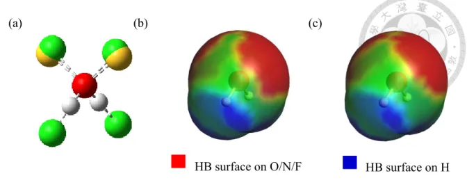
Instead of differentiating the hydrogen bonding surfaces, Chen and Lin [12] proposed to restrict the hydrogen bonding segments to those lying in the direction of lone pairs of the donor atoms (e.g., O, N, and F) and the OH, NH, and FH bonds. The lone pair vector, determined based on the VSEPR theory, and OH, NH, and FH bond vectors are used to find a hydrogen bond center (hbc) on the molecular surface, as shown in Figure 2.2-1 (a).
Furthermore, the HB-surface regions are identified as those located within a certain cutoff distance (RcutHB) of the hydrogen bond center, as shown in Figure 2.2-1 (b) and (c).
(a)
(b)
(c)
-0.025 -0.025 e/Å2
With the directional hydrogen bonding approach, the strength of segment interactions is then determined as the following:
ΔW(σm, σn) = (AES + BES
T2 )(σm + σn)2+ Chbmax[0, σacc - σhb]min[0,σdon + σhb] (2.2-9)
Note that the temperature dependence is introduced (as in the 2010 model) and the form of the hydrogen bonding interaction is the same as in the original model. After applying this modification in describing hydrogen bonding interactions, progress has been made.
In addition, it is worth to mention that the number of adjustable parameters is actually decreased, compared with the 2010 model. (see Table 3.1-1)
Rather than using the VSEPR theory, here we propose to use the MESP to determine the lone pair direction [34, 37-40]. The vector pointing from the donor atom to the local minimum in the MESP is considered as the lone pair direction, and its intersection on the molecular surface is the hydrogen bond center. The local potential minima can be found by searching the values in the potential field determined in quantum chemical calculations (evaluated on a 3-dimensional spatial grid). Each of the local minima found is regarded as a lone pair site. All other subsequent calculations are the same as those in the VSEPR approach (illustrated in Figure 2.2-2).
HB surface on O/N/F HB surface on H
(a) (b) (c)
Figure 2.2-2 (a) The hydrogen bond centers found by VSEPR and MESP for water. The green balls stand for the hydrogen bond centers from MESP while the yellow balls stand
for that in VSEPR. (b) The HB surface region of water from COSMO-SAC (DHB)/VSEPR. (c) The HB surface region within RcutHB water from COSMO-SAC (DHB)/MESP. Note that the hydrogen bond centers for proton donors are unchanged
since the only difference between the two methods is in the treatment of proton acceptors.
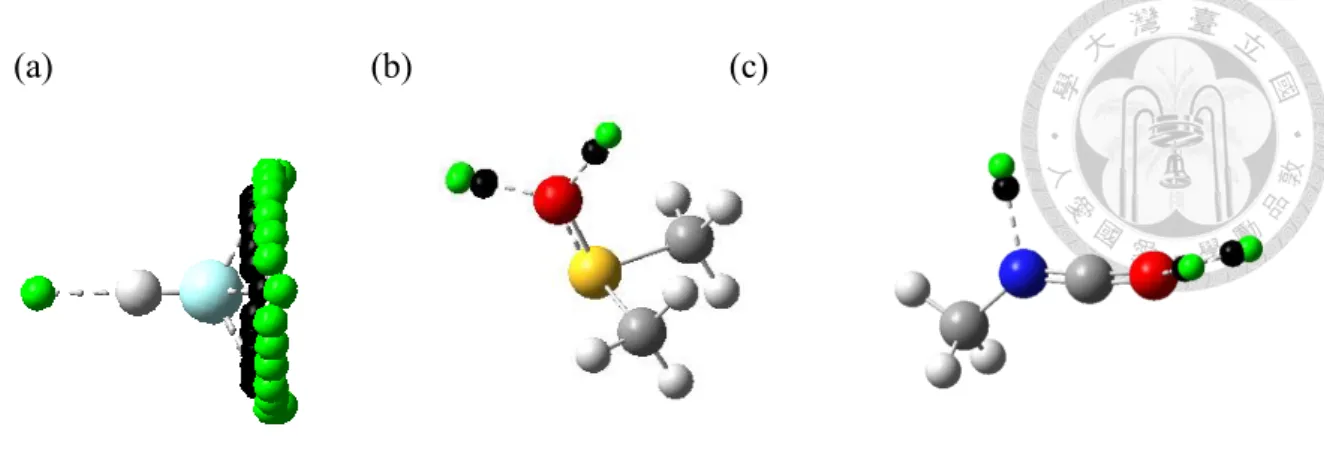
One advantage of MESP over VSEPR in determining the lone pair vector is illustrated in Figure 2.2-3 for HF, DMSO and methylisocyanate. For these compounds, it is not able to obtain the specific lone pair vectors by VSEPR. Through MESP, one can obtain lone pair directions without any auxiliary bond directions. More details about auxiliary bond directions and the difficulty of arranging lone pair positions are discussed in Appendix A.
The hydrogen bond centers determined from MESP for these compounds are illustrated in Figure 2.2-3.
(a) (b) (c)
Figure 2.2-3 The hydrogen bond centers determined from MESP for (a) HF, (b) DMSO and (c) methylisocyanate. The green balls stand for the hydrogen bond centers and the
black ones stand for electrostatic potential local minima found by MESP. The VSEPR fails to provide the lone pair direction for these compounds.
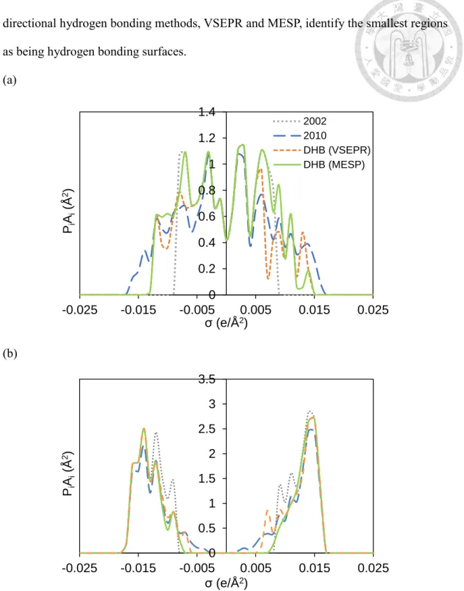
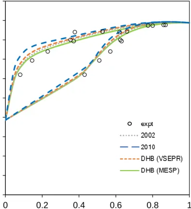
The difference in the treatment of hydrogen bonding segments is reflected in the σ-profile
“fingerprint” of the molecule. Figure 2.2-4 compares the water σ-profiles resulting from different COSMO-based models. To make it easier to recognize the different results of each COSMO-based models, the σ-profiles are separated into two parts, the contribution of non hydrogen-bonding segments (non hydrogen-bonding level σ -profile) and the contribution of hydrogen-bonding segments (hydrogen-bonding level σ -profile). Note that one can obtain the same σ-profile after sum up the two contributions for the same molecule. It can be seen that different treatments result in the same hydrogen bonding σ- profiles for extreme charge densities (e.g., |σ |00.016 e/Å2), indicating all 4 methods consider the most polarized segments as hydrogen bonding surfaces. At |σ| around 0.015 e/Å2, the 2002, VSEPR and MESP approaches identify a higher portion of surface regions as a hydrogen bonding surface. The most significant differences in the hydrogen bonding σ-profiles are observed for |σ|<0.014 e/Å2. In general, the 2002 treatment identify the
directional hydrogen bonding methods, VSEPR and MESP, identify the smallest regions as being hydrogen bonding surfaces.
(a)
(b)
Figure 2.2-4 σ-profile of water (a) non hydrogen-bonding level (b) hydrogen-bonding 0
0.2 0.4 0.6 0.8 1 1.2 1.4
-0.025 -0.015 -0.005 0.005 0.015 0.025
PiAi(Å2)
σ (e/Å2)
2002 2010
DHB (VSEPR) DHB (MESP)
0 0.5 1 1.5 2 2.5 3 3.5
-0.025 -0.015 -0.005 0.005 0.015 0.025
PiAi(Å2)
σ (e/Å2)
2.3 The Pitzer-Debye-Hückel Model
The activity coefficient of ILs can be considered to have contributions from short-range interactions and long-range electrostatic interactions. The short-range interactions are described by the COSMO-SAC model while long-range interactions are described by the Pitzer-Debye-Hückel (PDH) model [59, 60].
lnγi = ln 𝛾𝑖𝐶𝑂𝑆𝑀𝑂−𝑆𝐴𝐶+ ln 𝛾𝑖∗𝑃𝐷𝐻 (2.3-1)
where γi stands for the activity coefficient of species i in the solution. The long-range electrostatic contribution to activity coefficient is described by the PDH model as
ln 𝛾𝑖∗𝑃𝐷𝐻 = −√𝑀1
𝑠̅𝐴𝜙[2𝑧𝑖
2
𝜌 ln(1 + 𝜌𝐼𝑥
1 2) +𝑧𝑖
2𝐼𝑥 1 2−2𝐼𝑥
3 2
1+𝜌𝐼𝑥 1 2
] (2.3-2)
where 𝑀𝑠̅ is the molecular weight of solvent, 𝑧𝑖 is the electrovalence of species i, 𝜌 is the closest approach parameter, 𝐼𝑥 is the ionic strength that defined as
𝐼𝑥 =1
2∑ 𝑥𝑖 𝑖𝑧𝑖2 (2.3-3)
and 𝐴𝜙 is the Debye-Hückel constant that can be determined from 𝐴𝜙 =1
3√2𝜋𝑁𝑎𝑑𝑠̅× ( 𝑒2
4𝜋𝜖0𝜖𝑠̅𝑘𝑇)
1.5 (2.3-4)
with 𝑑𝑠̅ being the density of solvent, 𝑁𝑎 the Avogadro’s number, 𝑒 the charge of an electron, 𝜖𝑠̅ the average dielectric constant of solvent, k the Boltzmann constant, and T the temperature in Kelvin. In this work, the closest approach parameter in Eq. 2.3-2 is calculated based on the approximate theory proposed by Pitzer and Simonson [61] with ion-pair formation parameter being 2.5 [62-64].
𝜌 = 2.5(𝑟++ 𝑟−)√𝑀2𝑒2𝑁𝑎𝑑𝑠̅
𝑠̅𝜖0𝜖𝑠̅𝑘𝑇 (2.3-5)
where 𝑟 is the radius of an ion and the subscripts stand for cation (+) and anion (-).
The reference state of charged species is selected to infinite dilution in solvent. Therefore, the short-range activity coefficient of ions needs to convert to the following.
𝛾𝑖 = 𝛾𝑖∗𝑃𝐷𝐻𝛾𝑖𝐶𝑂𝑆𝑀𝑂−𝑆𝐴𝐶
𝛾𝑖∞𝐶𝑂𝑆𝑀𝑂−𝑆𝐴𝐶 (2.3-6)
where subscript i is cation or anion and 𝛾𝑖∞𝐶𝑂𝑀𝑆𝑂−𝑆𝐴𝐶 is infinite dilution activity coefficient of species i calculated by COSMO-SAC.
2.4 A Thermodynamically Consistent Extended PDH Model for Ionic Liquid Systems
When the electrolytes are dissolved in a solution of mixture solvents, Chen and Song [65]
suggested to use the mole-fraction averaged properties from all neutral species for the molecular weight (M), density (d), and dielectric constant (𝜖) needed in the PDH model (Eqs. 2.4-1, 2.4-2, and 2.4-3)
𝑀𝑠̅ = ∑ 𝑥𝑖 𝑖𝑀𝑖 (2.4-1)
1
𝑑𝑠̅ = ∑ 𝑥𝑖
𝑑𝑖
𝑖 (2.4-2)
𝜖𝑠̅ = 1
𝑀𝑠̅∑ 𝑥𝑖 𝑖𝑀𝑖𝜖𝑖 (2.4-3)
where 𝑥𝑖 is the mole fraction and the summations run through all neutral species.
However, the activity coefficient thus obtained does not meet the Gibbs-Duhem (GD) relation (see Appendix B for details). Here we adopt a similar method proposed by van Bochove et al. [66], the derived the expressions of activity coefficient by introducing the averaged solvent properties in the expression of excess Gibbs free energy given by Pitzer
where 𝐺𝑒𝑥 is the excess Gibbs free energy of system and 𝑁𝑇 is the total mole number of a mixture. Different from the work of van Bochove et al., here we include all components in the solution for the solvent properties (Eqs. 2.4-1 to 2.4-3) and treat the closest approach parameter (Eq. 2.3-5) being concentration-dependent. The new expression for activity coefficient of each species is
ln 𝛾𝑖∗PDH,extd= 𝜕
𝜕𝑁𝑖(𝐺𝑒𝑥
𝑅𝑇)
𝑇,𝑃,𝑖≠𝑗 = −√𝑀1
𝑠̅𝐴𝜙(−4𝐼𝑥
𝜌(𝑀𝑖
𝑀𝑠̅
𝜖𝑖−𝜖𝑠̅
𝜖𝑠̅ − 𝑧𝑖
2
2𝐼𝑥) ln (1 + 𝜌𝐼𝑥
1 2) +
2
1+𝜌𝐼𝑥 1 2
(𝑧𝑖
2𝐼𝑥 1 2
2 − 𝐼𝑥
3
2(1 +𝑑𝑖
−1−𝑑𝑠̅−1
𝑑𝑠̅−1 +𝑀𝑖−𝑀𝑠̅
𝑀𝑠̅ +𝑀𝑖
𝑀𝑠̅
𝜖𝑖−𝜖𝑠̅
𝜖𝑠̅ ))) (2.4-5)
For ionic liquid, both cation and anion are assumed to have same properties when using Eq. 2.4-5. That is,
θ𝑐𝑎𝑖𝑜𝑛= θ𝑎𝑛𝑖𝑜𝑛 = θ𝐼𝐿 (2.4-6)
where θ can be M, d or ϵ. The dielectric constant for ILs is determined by
𝜖𝐼𝐿 = 832.09 × (1000𝑀𝐼𝐿)−0.701 (2.4-7)
which is recommended by Lee and Lin [53] based on Singh and Kumar’s measurements [67].
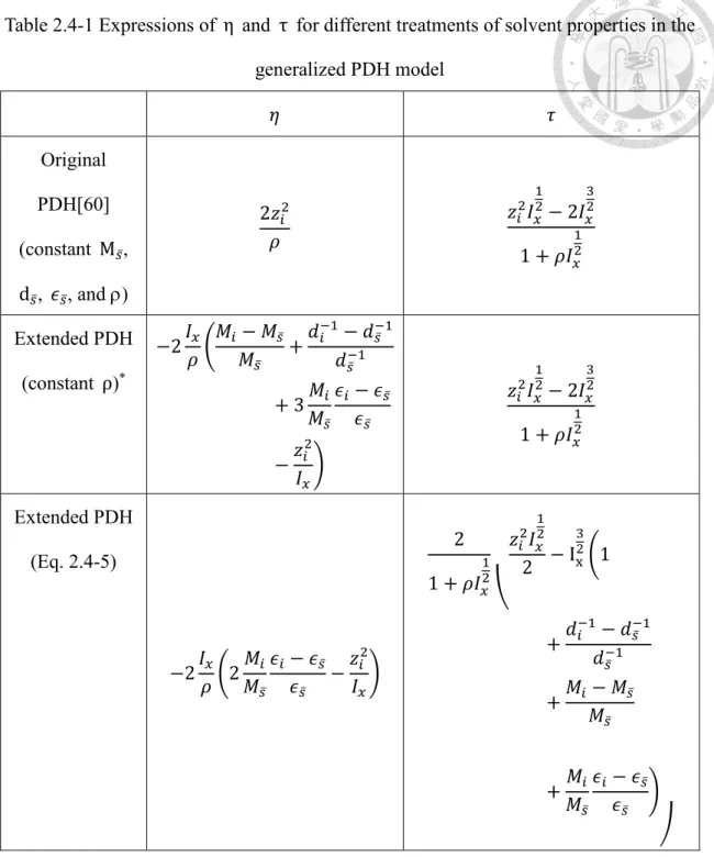
It is worth mentioning that the original and extended PDH models can be written in a general form that includes a term −√𝑀1
𝑠̅𝐴𝜙 followed by a logarithmic term with coefficient 𝜂 and a non-logarithmic term 𝜏, i.e.
ln 𝛾𝑖generalized PDH= −√𝑀1
𝑠̅𝐴𝜙(𝜂 ln (1 + 𝜌𝐼𝑥
1
2) + 𝜏) (2.4-8)
Table 2.4-1 summarizes the explicit forms of 𝜂 and 𝜏 of the two treatments on long- range interactions. Note that the extended PDH model (Eq. 2.4-5) reduces to the original PDH model (Eq. 2.3-2) in single solvent condition, i.e. θi= θs, where θ can be M, d or ϵ.
The examination of thermodynamic consistency of the PDH models is illustrated in Appendix B.
Table 2.4-1 Expressions of η and τ for different treatments of solvent properties in the generalized PDH model
𝜂 𝜏
Original PDH[60]
(constant M𝑠̅, d𝑠̅, 𝜖𝑠̅, and )
2𝑧𝑖2 𝜌
𝑧𝑖2𝐼𝑥
1 2− 2𝐼𝑥
3 2
1 + 𝜌𝐼𝑥
1 2
Extended PDH (constant ρ)*
−2𝐼𝑥
𝜌 (𝑀𝑖 − 𝑀𝑠̅
𝑀𝑠̅ +𝑑𝑖−1− 𝑑𝑠̅−1 𝑑𝑠̅−1 + 3𝑀𝑖
𝑀𝑠̅
𝜖𝑖 − 𝜖𝑠̅
𝜖𝑠̅
−𝑧𝑖2 𝐼𝑥)
𝑧𝑖2𝐼𝑥
1 2− 2𝐼𝑥
3 2
1 + 𝜌𝐼𝑥
1 2
Extended PDH (Eq. 2.4-5)
−2𝐼𝑥 𝜌 (2𝑀𝑖
𝑀𝑠̅
𝜖𝑖 − 𝜖𝑠̅
𝜖𝑠̅ −𝑧𝑖2 𝐼𝑥)
2 1 + 𝜌𝐼𝑥
1 2
( 𝑧𝑖2𝐼𝑥
1 2
2 − Ix
3 2(1
+𝑑𝑖−1− 𝑑𝑠̅−1 𝑑𝑠̅−1 +𝑀𝑖 − 𝑀𝑠̅
𝑀𝑠̅
+𝑀𝑖 𝑀𝑠̅
𝜖𝑖 − 𝜖𝑠̅
𝜖𝑠̅ ) )
*This is the result of the extended PDH model with the assumption of constant closest approach parameter (). The model of van Bochove et al. [66] would be identical to this model when all components in the solution are included as the solvent.
2.5 Partial Dissociation of Ions with Consideration of Chemical Reaction
According the work conducted by Lee and Lin [54] and the corresponding evidence by Nordness et al. [68], the IL molecule may partially dissociated. That is, dissociated ions (C+ and A-) and non-dissociated pairs (CA) will coexist and this can be described by a chemical reaction with equilibrium constant Ka .
𝐶++ 𝐴− ↔ 𝐶+𝐴− (2.5-1)
The equilibrium constant is the quotient of the activity (a) of 𝐶, 𝐴 and 𝐶𝐴.
𝐾𝑎 = 𝑎𝐶𝐴
𝑎𝐶𝑎𝐴=𝑥𝐶𝐴𝛾𝐶𝐴
𝑥𝐶𝑥𝐴𝛾±2 (2.5-2)
where γ±= √γC𝛾𝐴 is the mean activity coefficient.
The mole fraction of each component can be computed from a non-dissociated system 𝑥𝑠0 and 𝑥𝐶𝐴0 (𝑥𝑠0+ 𝑥𝐶𝐴0 = 1) and the degree of dissociation (α).
𝑥𝑠 = 𝑥𝑠0
1+𝛼𝑥𝐶𝐴0 (2.5-3)
𝑥𝐶𝐴 = 𝑥𝐶𝐴0 (1−𝛼)
1+𝛼𝑥𝐶𝐴0 (2.5-4)
𝑥𝐶 = 𝑥𝐴 = 𝑥𝐶𝐴0 𝛼
1+𝛼𝑥𝐶𝐴0 (2.5-5)
In pure IL systems, the equilibrium constant becomes 𝐾𝑎 =(1−𝛼0)(1+𝛼0)
𝛼02
𝛾𝐶𝐴
𝛾±2 (2.5-6)
where 𝛼0 is the degree of dissociation of pure IL (𝑥𝑠0 = 0) and is set to be 0.35 suggested by Lee and Lin [54].
Chapter 3. Computational Details
3.1 Information of Quantum Chemical Calculations
The Amsterdam Density Functional (ADF) software [69-71] is used to perform all QM calculations. The equilibrium geometry of a molecule is obtained using the GGA Becke Perdew functional and TZP basis set. The spatial distribution of the electrostatic potential is then calculated (using the “densf” utility) on Cartesian grids with medium resolution.
A local minimum in the MESP is determined by comparing the value at a grid point (located at the center of a local 3×3×3 grid) with its 26 neighboring grid points. Each of the local minima found is regarded as a lone pair site. The COSMO [72] calculation is then performed to obtain screening segment charge density on the molecular surface. For neutral species, the results of COSMO calculations have been done according to ADFCRS-2010 database [73-75] and we adopt the results inside the database. The calculation procedure for the activity coefficient is the same as that in the previous work [12].
In order to evaluate the performance of the COSMO-SAC model among different quantum calculation methods, it is necessary to re-optimize the parameters in COSMO- SAC. As in our previous work [15], fpol is the first parameter to optimize based on internal consistency for the averaging process. Second, we optimized the parameters in COSMO-SAC 2002, aeff and Chb, to fit VLE data for 1118 binary systems. Third, the five parameters in COSMO-SAC 2010, AES and BES, were fitted to LLE of 71 non-HB binary systems, and the HB interaction parameters, COH-OH, COT-OT and COH-OT were fitted to 309,
mixtures that contain hydrogen bond interactions (e.g. water, alcohols and amines). The objective function to be minimized, based on root mean square (RMS) errors for the VLE data, is given in Eq. 3.1-1 below.
RMSVLE = 1
M[∑ (yMi=1 icalc-yiexpt)2]
0.5+ 1
M[∑ (picalc-pi
expt piexpt )
2
Mi=1 ]
0.5
(3.1-1)
where y and p are the mole fraction and pressure in the vapor phase respectively, the superscript expt and calc stand for experimental data and calculated values, and M is the number of data points.
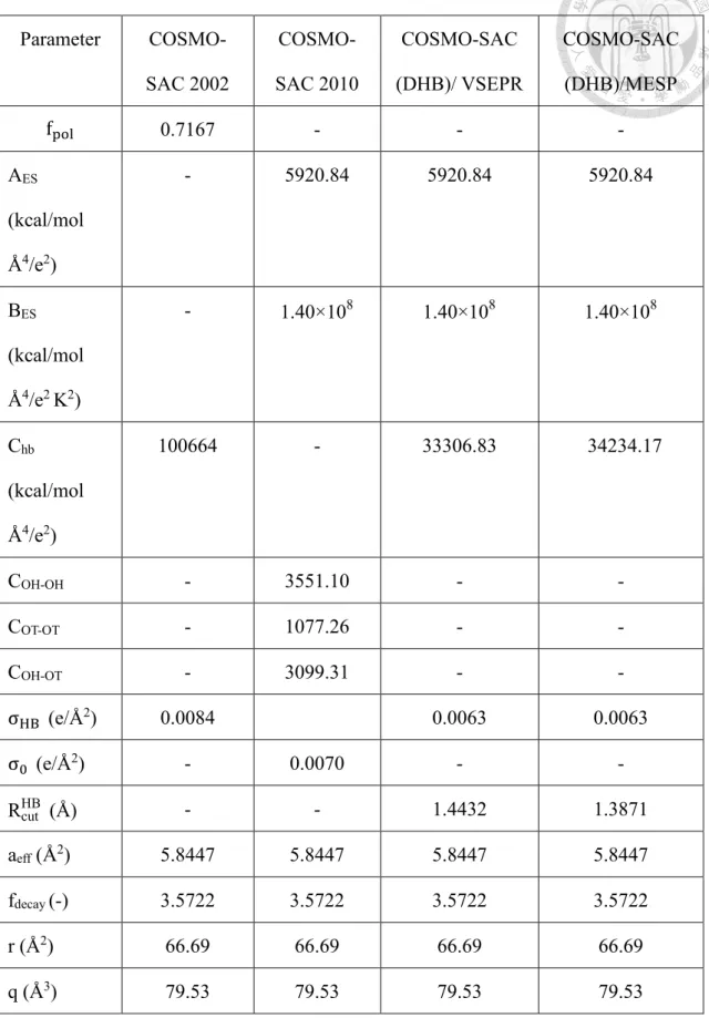
The re-optimized parameters for different variations of the COSMO-SAC model are summarized in Table 3.1-1.
Finally, the liquid-liquid equilibrium (LLE), the infinite dilution activity coefficients (IDAC) and octanol-water partition coefficients (Kow) are used to assess the predictive ability of the two types of COSMO-SAC (DHB) models. The experimental data for VLE, LLE and IDAC were obtained from the DECHEMA Chemistry Data Series [76] while the Kow data were obtained from the CRC handbook [77].
Table 3.1-1 Parameters in different COSMO-SAC models considered in this work.
Parameter COSMO- SAC 2002
COSMO- SAC 2010
COSMO-SAC (DHB)/ VSEPR
COSMO-SAC (DHB)/MESP
fpol 0.7167 - - -
AES
(kcal/mol Å4/e2)
- 5920.84 5920.84 5920.84
BES
(kcal/mol Å4/e2 K2)
- 1.40×10⁸ 1.40×10⁸ 1.40×10⁸
Chb
(kcal/mol Å4/e2)
100664 - 33306.83 34234.17
COH-OH - 3551.10 - -
COT-OT - 1077.26 - -
COH-OT - 3099.31 - -
σHB (e/Å2) 0.0084 0.0063 0.0063
σ0 (e/Å2) - 0.0070 - -
RcutHB (Å) - - 1.4432 1.3871
aeff (Å2) 5.8447 5.8447 5.8447 5.8447
fdecay (-) 3.5722 3.5722 3.5722 3.5722
r (Å2) 66.69 66.69 66.69 66.69
q (Å3) 79.53 79.53 79.53 79.53
3.2 Three Schemes for Degree of Dissociation of ILs
In this work, we examine three possible schemes of IL dissociation, as shown in Table 3.2-1, in the following discussion.
Table 3.2-1 The three schemes discussed in this work.
Scheme Dissociation Extent (α)
Number of components
Components involved
Non-dissociation 0 2 Solvent, IL ion pair
Full dissociation 1 3 Solvent, cation, anion
Partial dissociation determined based on Eq. 2.5-2 with α0 = 0.35
4 Solvent, cation, anion, IL ion pair
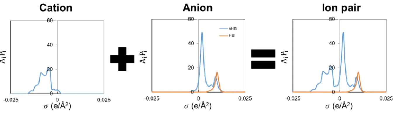
3.3 Combination of COSMO Files for Ion Pairs
For generating COSMO file of ion pairs, instead of directly calculating the ion pair structures in quantum mechanical calculation, we chose to first calculate the σ-profile of both the anion and the cation respective, and then combine them to represent the ion pair, as shown in Figure 3.3-1. This approach allows us to lower the computational cost in DFT, and was proven to be feasible in previous work by Lee and Lin [54].
Figure 3.3-1 Combination of σ-profiles of cation and anion for ion pairs
Chapter 4. Improved Directional Hydrogen Bonding Interactions for the COSMO-SAC Model for Prediction of Activity Coefficients
4.1 Comparison of Thermodynamic Properties from COSMO-SAC (DHB) Using MESP versus VSEPR
The VLE is commonly used to examine the performance of different models over the entire concentration range. The accuracy of VLE is evaluated by the average absolute relative deviation in vapor pressure (AARD-P) and average absolute deviation in mole fraction in the vapor phase (AAD-y). Eqs. 4.1-1 and 4.1-2 show the definition of AARD- P and AAD-y, respectively.
AARD-P = ∑ N1(M1
i∑Mj=1i |pcalcp- pexpexpt|) × 100%
Ni=1 (4.1-1)
AAD-y = ∑ N1(M1
i∑ |yMj=1i icalc - yiexpt|) × 100%
Ni=1 (4.1-2)
where N is number of VLE mixtures and Mi is the number of data points in the ith mixture.
The results are summarized in Table 4.1-1.
Table 4.1-1 Prediction accuracy of COSMO-SAC models for VLE, LLE, IDAC and Kow
VLE LLE IDAC Kow
AARD- P (%)
AAD-
y (%) RMSLLE Npts Nsys RMSIDAC RMS COSMO-SAC
2002 7.92 3.06 0.0776 2080 143 0.669 0.480
COSMO-SAC
2010 6.08 2.67 0.0929 2389 164 0.795 0.698
COSMO-SAC (DHB)/VSEPR
6.26 2.67 0.0933 2345 164 0.587 0.480
COSMO-SAC
(DHB)/MESP 5.80 2.53 0.0932 2393 167 0.598 0.462 Number of
binary pairs 586 190 431 291
The performance in VLE from different models falls in the order COSMO-SAC (DHB) based on MESP, COSMO-SAC 2010, COSMO-SAC (DHB) based on VSEPR, and COSMO-SAC 2002. The overall AARD-P from COSMO-SAC (DHB)/MESP is improved by 26.8%, 4.61% and 7.35% compared to COSMO-SAC 2002, COSMO-SAC 2010 and COSMO-SAC (DHB)/ VSEPR, respectively. As for AAD-y, it is reduced by 17.32% in comparison with COSMO-SAC 2002 and 5.24% in MESP compared with both COSMO-SAC 2010 and COSMO-SAC (DHB)/VSEPR. There is a substantial improvement in AARD-P, which indicates that COSMO-SAC (DHB)/MESP is much more successful in predicting vapor pressures.