黃銅退火雙晶與機械雙晶之顯微組織研究

(1)

國立臺灣大學工學院材料科學與工程研究所碩士論文

Graduate Institute of Materials Science and Engineering College of Engineering

National Taiwan University Master Thesis

黃銅退火雙晶與機械雙晶之顯微組織研究

Studies on Microstructure of Annealing Twin and Deformation Twin in α-brass

張以澄 I-Cheng Chang

指導教授：楊哲人博士 Advisor: Jer-Ren Yang, Ph.D.

中華民國 101 年 7 月

July 2012

(2)

i

誌謝

感謝指導教授楊哲人老師，您自大學時代的提攜促成我今日完成的學業，

學生會謹記您研究上嚴謹的態度，並致上最高的謝意，感謝您的教導。

感謝林新智老師、王星豪老師、以及黃慶淵學長對敝人論文上的指點，因為您們的建議，文章才得以更加完善，也許還有些不完美之處，但我會帶著您們的叮嚀，給予往後的研究或是工作上多些謹慎小心。

感謝我的父母、我的親人，因為你們在生活上給我足夠的支持，我才可以毫無後顧之憂完成學業，這段旅程暫時要寫下分號，新生活就要開始，我會好好照顧自己，不讓你們擔心。

感謝實驗室這幾年的陪伴，顏鴻威學長對研究的熱誠總令我深感佩服，您給我的建議一直是完成這本論文的動力，敝人不才，無法將您的想法發揮得更臻完善；謝謝李欣怡學姐自我大學時代指點我做實驗的技巧，同時也解答我許多研究上的疑惑，以後也許難以見面，希望您能夠好好保重身體。黃柏銘學長、陳苡諺學長要繼續好好相處，許正勳學長、張雅齡學姐在實驗上提供的協助，陳柏宇學長、王廷玉學長對實驗給的意見，張孝慈學姐在生活上提供的協助，陳孟揚學長雖然遠在法國，以後不再見面，也請多多保重，蔡宇庭要繼續加油。蔡宜良學長、

陳申賀學長、黃俊源學長雖然已離開實驗室，但謝謝你們在我碩一生涯填補些空缺，陳信良學長妙語如珠，希望你生活也能平安。同期的王惠琴、朱家瑋，謝謝你們在實驗上以及生活上給予的協助，往後的日子也要多多保重，希望我們三人都能夠有自己想要的未來。

系辦的林由莉小姐，謝謝你這六年來在生活上為我們打點一切，尤其是在完

成論文的這個階段，幸虧有您的提醒才不至有悲劇發生。謝謝陳學人先生在TEM

上的指導，以及容忍我的天兵。材料系 B95 的各位，幸虧認識你們，讓我初來台

北此地人生地不熟之餘感受到人情溫暖，你們在生活上的協助以及調侃是讓我進步的最大動力，謝謝這段日子個個所作所為才能造就今天的我，我們每人的際遇都不同，希望以後還有機會在某地相逢。林招松老師在我大學最困惑的時候給予

(3)

ii

多種意見，您就像父親會時時叮嚀我們每一人，謝謝您，我會去找最適合我的道

路。在此也要特別感謝成大的陳志慶學長以及黃俊銘學長在EBSD 上給予的協助，

使這論文能有初步的結果。

台大佛朗明哥舞社的各位，大家以後也要努力練舞。迷火的徐曉瑩老師、陳宇萍老師、張曉芸老師、黃譓容老師，尤其是陳筱晴，我的啟蒙老師，賽米亞的李容棻老師，陳雅惠老師，米拉索的蔡明娟老師以及陳志遠老師，從你們身上不僅學到舞蹈的技巧及身段，還有生活及做人處事態度。在台北的佛朗明哥圈認識的各位，謝謝你們在這幾年給的歡笑以及鼓勵，大家要繼續一起練舞，週一晚班及週二晚班的朋友對不起，沒能繼續上課，但我忘不了課堂結束後那些酒的滋味，

週六長尾裙班，我們要繼續努力，變成美人魚。《一個人。旅行》的好搭檔們：世

芳、美綸、曉芬、君潔、怡珍，要再同台一次也許不可能，這段練習的時光我會好好珍惜的。

徐禎，把你放在最後不是不看重你，而是這六年來除了家人外最親近的人就是你了，這些影響實在無法一一述說，但若沒有你的協助，我的生活不可能如此令人滿意，謝謝你。

總算完成了學業，感激之情卻又辭不達意。只能說：謝謝各位。

(4)

iii

中文摘要

雙晶是指材料中兩個晶體其方位具有鏡面對稱關係。此論文將針對以下兩種型態的雙晶加以討論：退火雙晶發生在退火時再結晶成長過程中，偶發的堆疊錯誤造成，而機械雙晶則是當基地受到應力應變，為了減少系統總能而產生。較早期的文獻認為機械雙晶僅僅發生在體心立方晶體內，但近期的實驗證明面心立方晶體中不僅有退火雙晶，也可能產生機械雙晶；因此，此篇論文中將介紹較廣為接受的理論及模型來解釋退火雙晶以及機械雙晶的生成原因。

由於雙晶晶界是由Shockley 部分差排以及疊差生成，在某些情況下可以阻礙

差排的前進，其往往被視為增強材料機械性質的要素之一；但有時候在雙晶介面附近會有差排滑移現象，因此雙晶材料的延展性可比其他加工硬化材料來得佳。

若雙晶晶界附近產生滑移，差排分解成部分差排，則僅有特定方向的部分差排可以繼續往前滑動，晶界會阻礙剩下的差排，因此晶界處會有階梯狀特徵。實驗中我們將以光學顯微鏡以及穿透式電子顯微鏡來觀察退火雙晶、機械雙晶、階梯狀特徵、滑移現象。

此外，本實驗也以電子背向散射繞射儀進行退火雙晶結晶面方位分析，同時

以矩陣來計算晶體之間的 misorientation；最後利用電子背向散射繞射的結果，施

打不同方位的結晶面硬度，以及不同結晶面之間的雙晶晶界硬度。

關鍵字：退火雙晶；機械雙晶；黃銅；Misorientation；電子背向散射繞射；穿透式電子顯微鏡

(5)

iv

ABSTRACT

The term of twin in materials represents two crystals with a mirror symmetry relationship. In this thesis, two types of twins will be discussed: one is the annealing twin, and the other is the deformation twin. The formation of annealing twin, as a result of annealing treatment, can be traced back to growth accidents or stacking faults during recrystallization. The deformation twin, on the other hand, is the accommodation to the deformation in matrix owing to the energy minimums. Additionally, some previous studies show that not only in BCC materials but also in FCC materials do deformation twins exist. Some conceivable models and mechanisms will be presented for the formation of annealing twins and deformation twins.

The twin boundary, formed by Shockley partial dislocations and stacking faults, is believed to enhance the mechanical property of materials because it can obstruct the movement of dislocations; therefore, the interaction of them and the incoming dislocations are noticeable. However, not every twin boundary will hinder the dislocation; unlike other strengthening method, the existence of twin boundary will improve the ductility. Some of dislocations may cross-slip at the twin boundary, and thus the ductility is maintained. One of the trace of cross-slipping is the ledge of twin.

When dislocation dissociates into Shockley partials, only part of incoherent twin boundary can glide continuously, while the other part stops and forms a “step” on boundary. In this thesis, the morphology of annealing twin, deformation twin, the ledge, cross-slipping will be shown by optical microscopy and transmission electron microscopy.

(6)

v

Besides, the orientation of annealing twins will be manifested by EBSD, and the identification of misorientation will be identified by orientation matrices. The result of EBSD will be used in the hardness test, which considers the effect of twin boundary in different orientation.

Keywords: Annealing Twin; Deformation Twin; Brass; Misorientation; EBSD; TEM

(7)

vi

LIST OF FIGURES

Fig. 2-1 Formation of an annealing twin by the nucleation on a close packed plane (a, b) [4]. ... 5 Fig. 2-2 Sequence of a close packed plane in FCC structure and in the related twin;

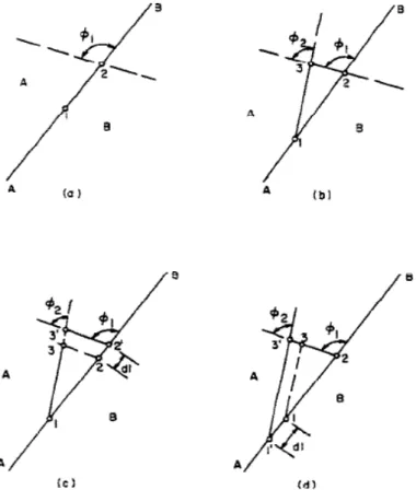
the coherent twinning plane refers to the close packed plane [4]. ... 5 Fig. 2-3 Left: Angles at junction of the twin boundary and the grain boundary. Right:

Schematic of change in boundaries as junction B move to C [7]. ... 6 Fig. 2-4 Initiation of twin formation when adjacent grains A and B have twin

orientation. [5] ... 8 Fig. 2-5 Twin initiates when adjacent grain boundary decomposes into “special

boundary.” [5] ... 9 Fig. 2-6 Schematic representation of coherent twin boundary formation in the grain corner. [3] ... 9 Fig. 2-7 (a) A 3-D representation of triangular nucleus. (b) Popping out of incipient twin along one portion of grain boundary. [5] ... 11 Fig. 2-8 Complex array of stacking faults which could act as a nucleus of twin

containing three {111} planes [7]. ... 11 Fig. 2-9 Relationship between twin width and grain size. [10] ... 12 Fig. 2-10 Left: schematic showing of a {111} step, i.e. MNRQ. Right: The

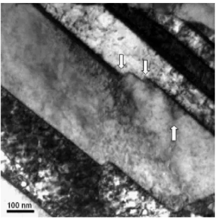
termination of Shockley partial loops on a migrating grain boundary [8]. .. 13 Fig. 2-11 Ledges at interfaces only a few nanometers wide [20]. ... 16 Fig. 2-12 TEM for the displacement of coherent twin boundaries resulting in steps and

(11)

x

jogs. [22] ... 16 Fig. 2-13 Surface Structure forming a grain boundary. (G.B.= Grain Boundary, G.S.=

Grain Surface, G= Grain) [2] ... 17 Fig. 2-14 (a) 3D view of partially grown annealing twin band and morphologies. The appearance of twin in 2D depends on the sectioning plane. (b) Grain corner twin, where C.T.B. means coherent twin boundaries, (c) complete parallel sided twin, (d) incomplete parallel sided twin. [5] ... 17 Fig. 2-15 Schematic showing various morphologies of annealing twins in FCC

structure [8]. ... 19 Fig. 2-16 Atomic structure of (112) deformation twin after volumetric deformation. [1, 2] ... 21 Fig. 2-17 The Thompson tetrahedron. [11] ... 21 Fig. 2-18 (a) Projection of ABCABCA….on {111} plane; (b) schematic of the

dissociation of AB dislocation according to the Heidenreich-Shockley mode;

(c) the corresponding edge-on view to (b); (d) schematic of that according to the Frank-Nicholas mode; (e) the corresponding edge-on view to (d) [21]. 23 Fig. 2-19 (a) An intrinsic stacking fault formed in a FCC crystal by removing part of a close-packed plane. (b) The addition of an extra close-packed plane to a FCC crystal produces an extrinsic stacking fault. [9] ... 24 Fig. 2-20 (a) AB is formed by the interacting attraction of the screw dislocation CA and BC; (b) Contracted and extend node configuration resulting from the dissociation of CA, BC, and AB dislocations into Shockley Partials; (c) Schematic of the situation that may exist during the formation of an intrinsic-extrinsic node pair; (d) Schematic of the configuration that may

(12)

xi

exist after the break-up of the four fold node. [2, 21]... 26 Fig. 2-21 (a) Planar view of a situation resulting from the dissociation of CA and CB

dislocations according to the Heidenreich-Shockley mode; (b)-(d) Schematics of the fault configurations which may evolve during the development of a fault-pair from the situation shown in (a); (e)-(h) Schematics of the corresponding edge-on views [21]. ... 28 Fig. 2-22 The Cottrel-Bilby pole mechanism for twinning in BCC crystals. [16]. ... 29 Fig. 2-23 Prismatic glide mechanism for FCC twinning [14]. ... 31 Fig. 2-24 Schematic illustration of the formation of a fault pair in FCC crystals. [19]33 Fig. 2-25 Micrographs of the contrast behavior of dislocations and faults observed of a twin F1 in a deformed Co-9.4wt% Fe alloy deformed 77K [15]. ... 34 Fig. 2-26 Schematic the formation of a fault-pair in the Ll0 structure [13]. ... 35 Fig. 2-27 Temperature-concentration diagram showing the occurrence of three modes of twinning propagation [12]. ... 36 Fig. 2-28 Micrographs of twinning types in (a) region I, (b) region II, (c) region III [12]. ... 37 Fig. 2-29 Electron micrograph showing twins is vertical to grains boundaries [18]. .. 42 Fig. 2-30 A generalized plot of twin density as a function of grain size [18]. ... 42 Fig. 2-31 The data of Bäro and Gleiter showing the relationship of twin density and temperature [17]. ... 45 Fig. 3-1 Schematic procedure of electrical polishing (a) the mounted specimen was chopped to expose the backside (b) the wire is attached and the backside is sealed before polishing. ... 52 Fig. 3-2 The schematic illustration showing the sampling of TEM specimens in

(13)

xii

deformed α-brass. ... 53

Fig. 3-3 (a) Rhombi at the {100} matrix and {110/100} twin boundary. (b) and (c) EBSD data show the grain orientation and Σ3 boundary. ... 53

Fig. 4-1 Optical metallographs resulting from annealing at 500℃ for (a) 1 h, (b) 2 h, (c) 3 h (d) 4 h, (e) 5 h, (f) 6 h, (g) 7 h, and (h) 8 h. . ... 57

Fig. 4-2 The relationship between grain size and twin thickness. ... 58

Fig. 4-3 Typical feature of annealing twin. ... 58

Fig. 4-4 5 pairs of coherent twin boundaries in a grain. ... 59

Fig. 4-5 Multiple twins cross in a grain of annealed α-brass, (a) for 8 h, (b) for 6 h. 60 Fig. 4-6 The ledges on the twin boundaries. Notice that some pointed out by arrows form with consecutive steps. ... 63

Fig. 4-7 TEM images of annealing twin boundary with a ledge. (a) Bright field (b) Drak field of annealing twin (c) Dark field of matrix (d) The selected area pattern and corresponding analysis. ... 64

Fig. 4-8 (a) Annealing twin with ledges at the corner of grain in compressed brass and the selected area diffraction pattern with corresponding analysis. (b), (c) The magnification of cross-slip at the annealing twin boundary, where (b) is the annealing twin boundary at position A and (c) is the junction at the position B. ... 66

Fig. 4-9 Schematic isometric grain with annealing twins inside of it, where is the average coherent twin boundary length. ... 71

Fig. 4-11 Relationship between twin density calculated by the interfacial area of twin boundary to the general boundary. ... 72 Fig. 4-10 Relationship between twin density calculated by twin number and grain size.

(14)

xiii

... 72 Fig. 4-12 Illustration of corner twin existence which only has one coherent twin

boundary. ... 73 Fig. 4-13 (a) EBSD data that the annealing twin with triangular shape in the middle of the picture. (b) The misorientation from orientation profile of the yellow, pink, and blue area are all 60°. ... 74 Fig. 4-14 (a) TEM image of annealing twin at the corner of the grain. (b) The selected area diffraction pattern and corresponding analysis. ... 74 Fig. 4-15 Illustration that two twins have the same surface area but the different

volume. ... 75 Fig. 4-16 (a) Two sets of electrons will be able to scatter inelastically at the Bragg

angle to a set of planes. (b)The electrons scattered inelastically in all directions will form a cone; the intersections of the cones and the image plane are Kikuchi lines. (c) Schematic Kikuchi bands formation in EBSD [6]. ... 86 Fig. 4-17 Geometry of the sample setup for EBSD measurement. ... 87 Fig. 4-18 The definition of the spherical Euler angles that describe an orientation of a crystal axes: X,Y, Z with respect to the sample axes: X’ (RD), Y’ (TD), Z’

(ND). (a) Crystal coordinate system. (b) The axes of sample rotate 1, Φ, and 2 about Z, X, and Z’ (ND) and the crystal frame is parallel to the specimen coordinate system.[24]. ... 87 Fig. 4-19 The EBSD of annealed α-brass reveals that there are 4 orientations inside of a grain and all of them have twin relationships and correlated Kikuchi patterns for (b) orange orientation, (c) green orientation, (d) purple

(15)

xiv

orientation, and (e) pink orientation. ... 88 Fig. 4-20 The orientation profile of Fig. 4-24(a) from the upper left corner to the

lower right one. It shows that all of the misorientation are 60° representing annealing twinning. ... 89 Fig. 4-21 The orientation profile of the lower left corner in Fig. 4-24(a), which shows the misorientation about 35°. ... 89 Fig. 5-1 Optical microstructures of homogenizedα-brass for 1 hour: (a) and (b)

undeformed structure, (c) deformed for 10% worked amount, (d) for 20%, (e) for 30%, while (e) for 40%. ... 92 Fig. 5-2 The microstructure of deformed 10% α-brass: (a) the grain boundary and the twin boundary are the hindrance of those sloped line, (b) and (c) are the magnification of (a) which show the sloped lines near grain boundary. ... 94 Fig. 5-3 Slip lines or deformation twins in the deformed annealing twin for 20%

work amount. ... 95 Fig. 5-4 (a) TEM bright field image of deformation twins within 40% work amount α-brass. (b) Bright field image of part of deformation twins. (c) The corresponding dark field. (d) The selected area diffraction pattern and the corresponding analysis. ... 97 Fig. 5-5 Typical morphology of deformation twins with 30% work amount under

TEM. (a) Bright field (b) Dark field (c) The selected area diffraction pattern and corresponding analysis. ... 100 Fig. 5-6 The stripes are obstructed by annealing twin boundary, and are cross to each other in 40 % worked amount.. ... 102 Fig. 5-7 (a) A TEM bright field image of deformation twins blocked by grain

(16)

xv

boundary. (b), (c) The dark field images of matrix at 111 M and deformation twins at 111 T. (d) The dark field at 111 M or 111 T. (e) The selected area diffraction pattern and corresponding analysis. The specimen is deformed by 20% work amount. ... 106 Fig. 5-8 (a), (b) TEM bright field image and corresponding dark field image of

deformation twins in annealing twin with 30% work amount. (c), (d) Bright field image and corresponding dark field image of annealing twin boundary which obstructs deformation twins. (e) The selected area diffraction pattern and correlated analysis. ... 107 Fig. 5-9 (a), (b) The bright field and dark field images of deformation twin with two orientation. The horizontal twins are formed first; the secondary twins cross-slip on them and also exist between original twins. (c), (d) The bright field and dark field images of intersected deformation twins. (e) The selected area diffraction pattern and corresponding analysis of matrix and two deformation twins. The specimen is deformed by 40% work amount.109 Fig. 5-10 (a) The bright field image of intersected deformation twins in 40% work amount α-brass. (b), (c) The dark field images of original deformation twins and secondary deformation twins, separately. (d), (e) The magnification of (a). Notice that there is some interruption at the intersection of two deformation twins. (f) The selected area diffraction pattern and corresponding analysis. ... 111 Fig. 5-11 (a) Stacking faults near the end of twins. (b) The selected area diffraction

pattern. ... 113 Fig. 5-12 The bright field images of stacking faults under two beam condition. ... 114

(17)

xvi

Fig. 5-13 Graphical change of the potential energy to the distance between atomic distance. ... 118 Fig. 5-14 Tensile test results of <100>, <110>, and <111> direction in FCC single

crystal metal [23]. ... 119 Fig. 5-15 The hardness plots with different grain orientation measurement. It is not

surprising that the hardness of {111} planes are the most high; on the other hand, {100} planes show the weakest mechanical property ... 120 Fig. 5-16 The hardness plots for twin boundary between different {grain/ twin}

orientation. ... 120 Fig. 5-17 The Hall-Petch plots with different grain size measurements. The result is compared to the work of Hsin-Yi Lee used different annealing times and temperatures [25]. ... 121 Fig. 6-1 (a) Undeformed α-brass with smaller grain size. (b) Deformed 30%. ... 125

(18)

xvii

LIST OF TABLES

Table 3-1 The reduced heights of α-brass and loadings... 52

Table 4-1 Experimental results of grain size and twin thickness. ... 55

Table 4-2 Experiment results of grain size, twin number per grain (NG), average coherent twin boundary ( ), and the interfacial area of twin per unit volume (Na) for different annealing times. ... 71

Table 4-3 Euler angles of each orientation. ... 81

Table 4-4 Axis/angle pairs of orange and green orientation ... 82

Table 4-5 Axis/angle pairs of orange and purple orientation ... 83

Table 4-6 Axis/angle pairs of purple and pink orientation ... 84

Table 4-7 Axis/angle pairs of different grains at lower left corner in Fig. 4-16(a). ... 85

Table 5-1 Hardness test results of different plane orientation. ... 118

Table 5-2 Hardness test of different twin boundary orientation. ... 118

(19)

1

Chapter 1 General Introduction

Twins are often a prominent feature in the material with low stacking fault energy.

Previous studies have indicated that that twin boundaries usually exhibit much lower energy and higher thermal stability compared with high-angle grain boundaries.

Moreover, they seem to possess rather superior fracture resistance and extremely low electrical resistivity. For example, Lu et al. [22] suggested that a reduction of neon-twin density for the same grain size result a noticeable decrement in rate-sensitivity and hardness. Systematic tensile tests and qualitative analysis also demonstrate that nanotwins would contribute to both strength and ductility. Thus, the mechanical property of twin boundary and twin formation are arisen much attention and the study has been investigated for decades.

The mechanism for the formation of annealing twins considers mostly two distinct concepts: (I) growth accidents, (II) nucleation of twins by stacking faults or fault packets, while for deformation twin, it usually relates to the stacking fault and the Shockley partial dislocation resulting from shear strain. However, there is still no general theory to describe the formation of annealing twin or deformation twin.

Therefore, some well-acceptable theories and models will be listed in Chapter 2, and the morphology of annealing twin and deformation twin will be shown in Chapter 4 and

(20)

2

Chapter 5, respectively. Furthermore, from the EBSD result in this thesis, the appearance of annealing twin is not always a lamellar structure. For accuracy, we will demonstrate the calculation of orientation matrix for annealing twin misorientation.

Additionally, the hardness test will also be presented to analyze the cross-slipping effect in twins.

(21)

3

Chapter 2 Literature Survey

2.1 Introduction of Annealing Twins

Annealing twins have been studied for over 80 years. They are observed in a variety of recrystallized FCC materials and exhibit some prominent morphologies, two long and parallel coherent boundaries with one or two ledges near grain boundaries.

Several proposed models have been attempted to address this issue and can be broadly classified to three groups [10]: (I) growth accidents [4, 26-31], (II) nucleation of twins by stacking faults or fault packets [5, 7], and (III) grain encounters [32-34]. The last model is not going to be discussed owing that there are some research suggest [35-38]

that twin is capable to form without two different grains “encountering” each other. To be short, grain growth accidents include that a coherent twin boundary forms at a migrating grain boundary due to an energetically favorable stacking fault. The second model illustrates that there is a kindly probability to form a twin nucleus when the grain boundaries migrate; furthermore, the twin grows by the glide of the incoherent twin boundaries. In the following sections, some well-accepted models in addition to the microscopic appearances of annealing twins would be presented literally.

(22)

4

2.1.1 The Growth Accidents Model

In 1969, Gleiter [4] developed a thorough model for the formation of annealing twins based on the concept of growth accidents. Gleiter [39] suggests that a boundary migrates through the way of atoms movement and deposition on a new plane. When a new atom packs on the surface, it inclines to deposit next to the boundary ledge or step for the surface energy minimum. As illustrated in Fig. 2-1, which shows a boundary is migrating; the grain (II) is growing and grain (I) is shrinking. Thus atoms on the boundary of grain (I) would move to that of grain (II), impinging on the close packed planes (ab, bf, etc). In the case of an FCC crystal, if the close packed plane ab is B layer, then the stacking atoms can go to the C or A sites as shown in Fig. 2-2. If the former takes place, then a perfect crystal with an FCC lattice is continued because {111} planes form an ABC-sequence as usual. However, if the atom arranges itself to A sites, then a twin orientation generates as the B layer is the twinning plane illustrated in Fig. 2-2

Once a wrong lattice position forms, the first layer of twin then is acquired.

The process is not continued until another faulted layer is produced; thus the distance of two mistakes can be treated as the width of twin. If there are only a few lattice planes between the two nuclei, a thin twin will exist.

(23)

5

2.1.2 Nucleation of Twins by Stacking Faults

Compared to the atomic model of Gleiter, Dash and Brown [7] had elaborated that the twin stems from a thermally activated diffusionless transformation. A twin region in two encountering grains is achieved if they lie close to the twin orientation [40];

Fig. 2-2 Sequence of a close packed plane in FCC structure and in the related twin; the coherent twinning plane refers to the close packed plane [4].

Fig. 2-1 Formation of an annealing twin by the nucleation on a close packed plane (a, b) [4].

(24)

6

therefore, twins nucleate at grain boundaries during recrystallization. Once stacking faults are generated, the single or complex array of those faulted planes will act as a nucleus of twin. While grain grows, the stacking faults or thin twins glide into the interior of grain from the boundaries. Based on their calculation as illustrated in Fig. 2-3, the sidewise growth (perpendicular to the coherent twin boundary BD) is dependent on the ratio of grain boundary energy to the increasing thickness, ΔS. However, the coherent twin boundary plays a minor role and does not contribute to the sidewise growth .

For the edgewise growth (along BD), the driving forces are the coherent twin boundary energy and other interfacial value, , where represents

Fig. 2-3 Left: Angles at junction of the twin boundary and the grain boundary. Right: Schematic of change in boundaries as junction B move to C [7].

D

(25)

7

the incoherent twin boundary energy, and are grain boundary energy and the surface energy of incoherent twin boundary energy, separately. For a spontaneous moving of the incoherent twin boundary moves into the grain, the reduction of grain boundary energy exceeds the increment of incoherent twin boundary energy. As the twin grows, the coherent twin boundary energy thus should not be dismissed due to the increase of coherent twin boundary.

Meyers and Murr [5] provided another aspect of the surface energy to describe the initiation and the propagation of twin. The model includes two parts, initiation and propagation. When two adjacent grains are close to twin orientation and the boundary inclines to random, the twin nucleus would form if the grain boundary 12 is replaced by the incoherent boundary 13 and coherent twin boundary 23, as illustrated in Fig.

2-4. The total system displays as:

(2.1)

Where represents the incoherent twin boundary energy of 13, while and are the coherent twin boundary energy and grain boundary energy, respectively. And

, , and represent the area of corresponding interfaces. After nucleation, the Shockley partial dislocations “pop out” of the boundary and propagate to the material which resulting in twin stacking fault sequence and minimal strain in the material coinciding with energy minimum, as showing in Fig. 2-4(c) and (d). The more

(26)

8

dislocations form or the farer they glide, the wider the twin nuclei are.

However, if two adjacent grains and their boundary are both at random orientation, a twin nucleus will generate (with respect to A) for the purpose of the interfacial energy

minimum. As shown in Fig. 2-5, 23 and 13 are coherent boundary and incoherent one with the boundary energies and , separately. The equation can be expressed as:

23 + 13 + 12 < γ12 (2.2)

The inequality suggests that it happens under the circumstances of < γ, and thus the “special” boundary does exist and replace the original boundary.

Fig. 2-4 Initiation of twin formation when adjacent grains A and B have twin orientation. [5]

(27)

9

Fig. 2-5 Twin initiates when adjacent grain boundary decomposes into “special boundary.” [5]

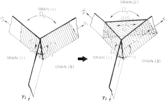
Fig. 2-6 Schematic representation of coherent twin boundary formation in the grain corner. [3]

Similar demonstration at triple junction [3] is shown in Fig. 2-6. To form a corner twin with the excess of twin boundary, the interfacial energy must be lower than the original one or the dihedral angle (Ω ) would become less than 120° [41]. This feature has been manifested by Fullman and Fisher [28] with optical metallographic measurement on annealed copper samples; moreover, Murr [42] also had shown the same observation about austenite under a transmission electron microscope.

(28)

10

As depicted in Fig. 2-7, 2365 and 1463 are the coherent and non-coherent twin boundaries, respectively. When propagating, the twin would grow through the migration

of the non-coherent boundary 1463. In Fig. 2-7 (b), the boundary 1 463 represents the moving non-coherent boundary. It must be noted that the mobility of coherent twin boundary is rarely low for the reason that since the coherent twin boundaries have relatively lower energy, their mobility perpendicular to the boundary is not expected to be as sufficient as of other random boundaries [27, 43]. Based on the grain boundary migration mechanism of Gleiter [39], the boundary moves faster with more steps for atom deposition. If the coherent twin boundary is regarded as theless-stepped boundary, its migration will not be as valid as other kinds of boundaries. Consequently, the distance of the coherent boundaries does not increase severely during the twin propagation.

Under the circumstances of recovery, the sweep-up inside the twin volume doesn’t provide the driving force until the system energy reaches the minimums. In the work of Dash and Brown [7] as mentioned before, the incoherent boundary are formed by an array of Shockley partial dislocations. These dislocations “pop out” of the grain boundary and dissociate to form stacking fault, and thus one or a packet of stacking faults form twin nucleus, which is illustrated in Fig. 2-8.

(29)

11

Fig. 2-7 (a) A 3-D representation of triangular nucleus. (b) Popping out of incipient twin along one portion of grain boundary. [5]

Fig. 2-8 Complex array of stacking faults which could act as a nucleus of twin containing three {111} planes [7].

(30)

12

What the description of dislocation movement from Mayers and Murr [5]

elaborating the propagation of twinning process is only focused on “the growth of twin”;

this does not explain sufficiently other phenomena of annealing twin, such as the rate of twin formation, twin density. Those phenomena may be clarified appropriately by dislocations. In reality, the growth of twin may be affected by many factors when annealed, which would be described in section 2.3.3. Nevertheless, the mechanisms in this section still agree to one of results from Pande. et al. [10]: there are some observations of the relationship between the width of twin and grain size, as in Fig. 2-9 [10]. This is because the larger the faulted packets, the greater the chance of another faulted plane will form adjacent and then the twin coalesce.

Fig. 2-9 Relationship between twin width and grain size. [10]

(31)

13

2.1.3 The Model Consisting of Partial Dislocations

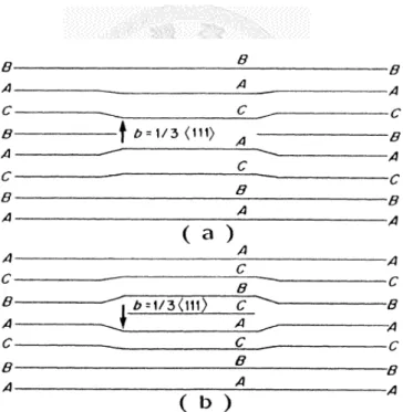
The model proposed by Mahajan [8] addressed another formation of annealing twin. It is based on four assumptions: First, the grain boundary must migrate. Second, the driving force for grain boundary migration depends on its curvature; the smaller the radius of curvature is, the higher the driving force should be applied. Third, the curvature of boundary can be described as facet or ledge. Finally, some of the steps lie on 111 . Similar to Gleiter [4], Mahajan et al. also proposed a model of the step at grain boundary. The faulted area, MNRQ, in the migrating grain (I) which is assumed that the grain (I) grows at the expense of grain (II), is bounded by a Shockley partial loop, in Fig. 2-10. Assuming that the grain (I) grows at the expense of grain (II), then the faulted area MNRQ of grain (I) is bounded by a Shockley partial loop.

Fig. 2-10 Left: schematic showing of a {111} step, i.e. MNRQ. Right: The termination of Shockley partial loops on a migrating grain boundary [8].

(32)

14

Basically, when the grain boundary moves forwards, the probability of ledge (111) become Shockley partial also increases; in other words, the number of twins increases with increasing grain size. However, this mechanism is contrary to that of Meyers and Murr [5]: dislocations are not opposite totally, such as δA and Aδ. The reason is that there is no driving force for the movement of such partial dislocations. The clearer identification of δA or Aδ may be referred to section 2.2.1 and 2.2.2.

On the right side of Fig. 2-10, there is an interesting inclining facet on the grain boundary. If one faulted layer forms, the subsequent layers will pile up as the schematic with Shockley partials loops P1, P2 and P3. For the sake of the energy minimum, the habit plane of the grain boundary may locally tilt where the twin meets the grain boundary.

To consider whether the twin forms or not, a general equation (2.3) expresses the interaction of driving force and the hindrance associated with a circular, one-layer twin of radius R.

∆E πRG (2.3)

Where G is the shear modulus, b is the Burgers vector of the bounding Shockley partial and γ is the stacking fault energy. According to equation (2.3), there are two reasons that the material could not form the twin in the high-stacking-fault-energy material.

(33)

15

First, if a material has a higher γ, it must have a low R to make ∆E reasonable, thus the low R may not reach the minimum size for a nuclei to form. The other reason is that Shockley partial loops may not be stable at high-stacking-fault-energy materials since the stacking fault energy is too high to make partials repel each other and glide away from the boundary to generate a twin. However, this rough estimation conflicts to the fact that there are twins which do exist in high stacking fault energy materials such as aluminum [44, 45]. It may imply that there are other restrictions to the formation of twin;

additionally, the nucleus of twin on the stacking fault may not be suitable to treat as a circular.

2.1.4 The Appearance of Annealing Twin

Consider a total dislocation 1 1 0 breaks down into a pair of partials in a FCC material [6], the dissociation is able to be written as

1

2 1 1 0 → 1

6 1 2 1 1

6 2 1 1 (2.4)

The additional plane between two dissociating partials becomes a stacking fault. In section 2.1.1, the model of Gleiter [4] has explained that the stacking fault is the result of misaligned atoms. Several electron microscopy observations [20, 22, 39, 46] (Fig.

(34)

16

Fig. 2-11 Ledges at interfaces only a few nanometers wide [20].

2-11 and Fig. 2-12) reveal that the steps-like structures are formed by the 111 planes of grain near grain boundaries, as the simple schematic diagram, Fig. 2-13.

Fig. 2-12 TEM for the displacement of coherent twin boundaries resulting in steps and jogs. [22]

(35)

17

Fig. 2-13 Surface Structure forming a grain boundary. (G.B.= Grain Boundary, G.S.= Grain Surface, G= Grain) [2]

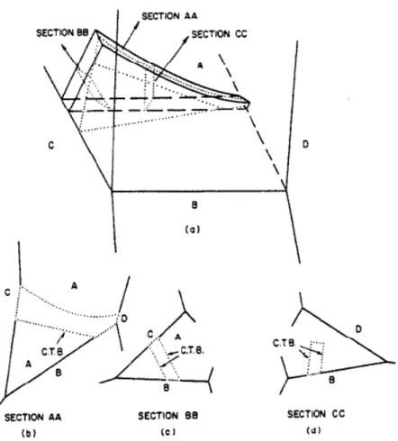
Fig. 2-14 (a) 3D view of partially grown annealing twin band and morphologies. The appearance of twin in 2D depends on the sectioning plane.

(b) Grain corner twin, where C.T.B. means coherent twin boundaries, (c) complete parallel sided twin, (d) incomplete parallel sided twin. [5]

(36)

18

Due to the giant volume of annealing twin, it is more appropriate to observe the appearance of annealing twins by the optical microscopy. It is important that the real shape of annealing twin is not lamellar or triangular but octahedron, which is relevant to four 111 planes in a FCC unit crystal and the innate of twinning plane as a role like a mirror. That is why the observation in two dimensions does not represent the real morphology. Those mentioned above can be rationalized by Fig. 2-14. If the observation plane under the optical microscopy is on the section AA, then a corner twin is observed.

Similarly, if the planes are on section BB or section CC, then the complete and incomplete parallel sided twin are observed, respectively.

Mahajan et al. [8] also proposed four prominent twin morphologies which schematically shown in Fig. 2-15: A corner twin is labeled by A and its coherent twin boundary produces a trace MN. Twin B is thin and seems to be through the whole grain, while twin C is thicker than twin B and end up within the grain. Finally, the twin D is shallowly inclined to the grain boundary. Imaging that a 111 step is migrating towards the grain corner and is close to a triple point of grain boundaries, the repulsive force will drive atoms to the other side of grain forming the twin A in the corner owing to the growth accident and the bounding partial with same burgers vector. The way that twin B forms also results from Shockley partial loops on a migrating grain boundary but

(37)

19

Fig. 2-15 Schematic showing various morphologies of annealing twins in FCC structure [8].

does not take place near the triple point. If it does, the situation would become like that of twin A. Comparing twin C with B, the former stunts right in the middle because the partial of different burgers vector bounds the growth of twin. The above morphologies have been also discussed by Meyers and Murr [5], but the last one is not rational according to their theory. The morphology of twin D can be explained by the theory of Gleiter [4]. If grain (I) grows towards grain (II) and growth accidents occur on the facet, the misalignment of atoms will not bring on a twin until another mistake arises; thus, an occluded twin forms. Furthermore, the nucleation and growth can take place easily on the steps of 111 planes [4, 39]; this feature is an significant ledge under the optical microscopy.

(38)

20

2.2 Introduction of Deformation Twins

Different to annealing twins, deformation twins are generated by mechanical stresses, sheer strains and dislocations. It [47] has long been considered as a product by the above influence in BCC, HCP, and lower symmetry metals and alloys [48-52]. But decades ago, it was also found in FCC metals and alloys [13, 53-55], ordered structures [56], intermetallic compounds [57], semiconductors [58] and compounds [59], some non-metallic compounds [60-62] like calcite and sodium nitrate [63-65], or even in complex minerals [66] and crystalline polymers [67, 68]. For simplification, the phenomenon of deformation twin is the coordinated and slight displacement of individual atoms in lattice: the atoms on the first layer of plane next to the twin boundary displace a unit length, which is quite small or a slip would take place, and those on the second layer move twice amount of the first layer, and so on [69], shown in Fig. 2-16. Most theories [13, 15, 19, 21, 44, 47, 48, 50, 56, 59, 70-75] imply that deformation twins with imperfect structures consist of many stacking faults; however, there has no general agreement on the mechanisms of deformation twins. In the following sections, some mechanisms would be applied and are concentrated on the high-symmetry structures.

(39)

21

2.2.1 The Thompson Tetrahedron for Dissociation of Dislocations

Fig. 2-17 The Thompson tetrahedron. [11]

Fig. 2-16 Atomic structure of (112) deformation twin after volumetric deformation. [1, 2]

(40)

22

The notation of Thompson tetrahedron, in Fig. 2-17, is effective to visualize the close-packed planes in FCC and diamond cubic materials. The four faces conceive four 111 planes of crystal which is unfolded on the image plane. The vertices of tetrahedron denotes as A, B, C, and D; D is above of the image plane where ABC lies on.

And the faces mid-points α, β, γ, and δ, are the opposite points of its vertex, A, B, C, D, respectively. The Burgers vectors of dislocations are specified by their two end points on the tetrahedron, and thus they could be defined as vectors on the tetrahedron both in magnitude and direction. So long as the Shockley partial dislocation dissociates, they would be constrained on the 111 planes and be represented by the lines from the corners to the center of the faces, Aβ, Aγ, etc. The dissociation of AB could be expressed alternatively as follows [11, 76]:

AB → Aδ +δB (2.5)

or

1

2 1 1 0 → 1

6 1 2 1 1

6 2 1 1 (2.6)

In FCC crystals, a total dislocation can extend in two different ways[21]. The first mode is of Heidenrich-Shockley [77], illustrated in Fig. 2-18(b) and (c). The feature is that dislocation with Burgers vector, AB, dissociates into two partials with Burgers vector Aδ and δB. If the partial with δB leads the other one with δA, then they will

(41)

23

result in an intrinsic stacking fault, …BACBCBAC….

The other mode is demonstrated in Fig. 2-18(d) and (e). On the contrary, if it is the Fig. 2-18 (a) Projection of ABCABCA….on {111} plane; (b) schematic of the dissociation of AB dislocation according to the Heidenreich-Shockley mode; (c) the corresponding edge-on view to (b);

(d) schematic of that according to the Frank-Nicholas mode; (e) the corresponding edge-on view to (d) [21].

AB

Aδ δB

AB

Aδ = δC + δB

δB = Aδ + Cδ

δB Aδ

δC Cδ

(42)

24

Fig. 2-19 (a) An intrinsic stacking fault formed in a FCC crystal by removing part of a close-packed plane.

(b) The addition of an extra close-packed plane to a FCC crystal produces an extrinsic stacking fault. [9]

partial with δA that leads δB, then an anomalous fault, …ACBAACB…, will generate.

However, it can be avoided if δB and δA can split into other partials:

δB → Aδ Cδ (2.7)

and

Aδ → δC δB (2.8)

As a consequence, it would lead to an extrinsic fault. The schematic of intrinsic and extrinsic faults can be referred to Fig. 2-19.

An example [78] is given to be clarified. For the dislocation with the Burgers

(43)

25

vector of 1 1 0 , first it may dissociate into 1 1 2 and 1 1 1 . If the former guides the latter, then there will be an intrinsic fault layer on 111 plane. On the other hand, if the latter leads the former, then there are two dissociations take place:

1

6 1 1 2 →1

3 1 1 1 1

6 1 1 4 (2.9)

1

3 1 1 1 →1

6 1 1 4 1

6 1 1 2 (2.10)

The partial dislocation 1 1 4 is referred to Cδ and its inverse is δC. Since this dislocation only sessiles, such an extension renders the dislocation incapable of glide.

Therefore, it is the Shockley partial 112 that decides the width of extrinsic fault plane owing to the ability to glide.

2.2.2 The Model of Node-Pairs and Fault-Pairs

Mahajan [21, 79] had purposed a dislocation model for the theory in the formation of deformation twin which has been observed by Loretto [80], Ivew and Ruff [73], Gallagher [81], and Gallagher and Washburn [82]. For the sake of simplicity, the involved dislocations are assumed to be pure screw, though most of dislocations are mixed. In the following Fig. 2-20(a), AB is a junction of BC and CA dislocations attracting to each other. As the envision of Thompson [83] and Whelan [84], those

(44)

26

perfect dislocations lying on the same plane not only dissociate into Shockley partials, but will construct a possible dislocation node as the configuration in Fig. 2-20 (b). On the right side of junction, these split partials can cancel in pairs near the node and produce an extended type, which is opposite to the other side that those partial contract with a node. The concept of node [83] is that a finite length of dislocation is anchored at its end, and rotates itself to generate a new dislocation loop per revolution.

Fig. 2-20 (a) AB is formed by the interacting attraction of the screw dislocation CA and BC; (b) Contracted and extend node configuration resulting from the dissociation of CA, BC, and AB dislocations into Shockley Partials; (c) Schematic of the situation that may exist during the formation of an intrinsic-extrinsic node pair; (d) Schematic of the configuration that may exist after the break-up of the four fold node. [2, 21]

AB

δB

δB \δB

Bδ

δB

Bδ

Bδ Aδ

Aδ Aδ

δA

δC δC

δC

δC δC

δC Bδ

Cδ

Cδ Cδ

Cδ BC

BC CA

CA

Cδ δA δB Cδ δA δB

Cδ

δA Bδ + Cδ δA Bδ+Cδ

Bδ = δA + Cδ Bδ = δA + Cδ

(45)

27

When the partials with Burgers vectors δC and Cδ move from right towards left, the partials with Burgers vectors δA and Bδ also glide through the plane as a pair;

ultimately, they bound together in a triangular shape. Once the partials with Burgers vectors δA and Bδ dissociate into the partials with Burgers vectors Bδ Cδ and δA δC likewise, respectively, there will be an extrinsic-faulted region as illustration in Fig. 2-20(c). The partial pair, Cδ and δC thus combine together and show an edge character which is perpendicular to δA and Bδ in the last illustration, Fig. 2-20(d), as an extending extrinsic stacking fault with the four-fold node.

Consider the interaction of dislocations with Burgers vectors CA and CB gliding on the same plane; Fig. 2-21(a) shows these two partials dissociate into δA Cδ and δB Cδ. Since δA and δB are attractive to each other, δB and Cδ may somehow recombine together into CB as shown in Fig. 2-21(b); on the contrary, the repelling partials δA and Cδ remain as the boundaries of an intrinsic stacking fault. If CB dislocation dissociates in such a manner that the partials with Burgers vector δB leading the partial δC, then δB will interact with δA in Fig. 2-21(c) and (d). As already noted above, the partials δB and δC then dissociate to form an extrinsic fault which will blend readily with the intrinsic fault and construct a fault-pair.

(46)

28

Fig. 2-21 (a) Planar view of a situation resulting from the dissociation of CA and CB dislocations according to the Heidenreich-Shockley mode; (b)-(d) Schematics of the fault configurations which may evolve during the development of a fault-pair from the situation shown in (a);

(e)-(h) Schematics of the corresponding edge-on views [21].

Cδ δA δB

Cδ δA δB δB = Aδ + Cδ

δB = Aδ + Cδ

δB = Aδ + Cδ δB

δB

Cδ Cδ

Cδ

Cδ Cδ

C\δ

Cδ Cδ

Cδ

Cδ Cδ

δA

δA δA

δA

δA Aδ δA

δA

δA CB

CB

a/√3

(47)

29

2.2.3 The Modified Models of Pole Mechanism

The formation of deformation twin involves not only the heterogeneous nucleation from the defect, but as the accommodation of the shear force on the lattice around the twin region. Cottrell and Bilby [16] considered a continuous growth of a BCC twin from the dissociation of a perfect dislocation in the parent lattice [19]. In Fig. 2-22, a portion OB of a perfect dislocation AOBC, having a Burgers vector 111 and lying on the (112) plane where it cannot glide, dissociates based on the following reactions with the nodes at O and B:

1

2 111 → 1

3 112 1

6 111 (2.7)

Fig. 2-22 The Cottrel-Bilby pole mechanism for twinning in BCC crystals. [16].

(48)

30

The Burgers vector of BDEO is 111 , and thus the partial dislocation glides in the (112) plane; while the other partial dislocation 112 is sessile and remains along OB.

Since BDEO is glissile, EO may lie on 111 direction and thus become pure screw in character, leading to a new twin type stacking fault on 121 or 211 . The reason based on the crystallography is that both of 121 and 211 are twinning planes intersecting 112 plane in 111 direction of BCC crystal.

Venables [14] suggested a modified mechanism for FCC crystals. With the utility of the notation of Thompson tetrahedron, a dislocation with Burgers vector AC lie on the plane (b) except for a long jog between the nodes, N1 and N2, on the plane (a). If the part of the dislocation dissociate into:

AC → Aα αC (2.8)

Or it may be given as

1

2 110 → 1

3 111 1

6 112 (2.9)

The Frank partial Aα, or 111 , sessiles on the plane (a) while the Shockley partial αC, or 112 , glides around the pole of dislocation AC, contributing an intrinsic stacking fault as depiction in Fig. 2-23(b).

Venables [14] also assumed that the partial αC recombines the sessile partial Aα

(49)

31

Fig. 2-23 Prismatic glide mechanism for FCC twinning [14].

plane (a)

AC

αC

along the length RN2 after a rotation. In Fig. 2-23(c), if two partials meet at RS with a separation of an interplanar distance, then a pole dislocation will form to transfer itself to the upper or lower plane between the jog and the plane (a), with a Burgers vector of 221 [85]. After that, the reformed dislocation with Burgers vector AC then glide to the next plane (a), leaving a jog, and then repeating the dissociation. Thus, the thickness of twin embryo increases steadily by repeated process of dissociation, rotation, and then displacement till the partials can pass. The illustrated T1 and T2 are twins which have helical stacking faults and are constructed by dislocations sources.

(50)

32

2.2.4 Theory of Twin Activated by Multiple Slip Systems

Later theories of deformation twinning in FCC materials suggest that it does not take place until at least two slip systems involved [47]. Mahajan and Chin [15] applied a mechanism of dislocation dissociation descripted as follows equation:

BC DC → 3αC ^(2.10)

Where BC is the primary system and DC is co-planar. The implication of equation (2.10) will be discussed in the latter paragraph.

Majajan [48] supposed that these two dislocations dissociate into Shockley partials, and glide on the same plane, as shown in Fig. 2-24(a). It is assumed that the dissociated Shockley partial Dα is prior to αC; moreover, to avoid high energy fault, Dα and αC are going to split as

Dα ⟶ αC αB (2.11)

and

αC ⟶ Bα Dα (2.12)

Thus as illustrated in Fig. 2-24(b), Dα and αC are transferred to the adjacent upper plane and the partials Bα and αB annihilate each other, resulting in an extrinsic faulted plane.

(51)

equa was will not

Fig.

in FC

However, ation (2.10),

derived fro generate thr sufficient t

2-24 Schem CC crystals.

it is not cl in spite of om a BCC ree success to exhibit

matic illustr . [19]

lear how th the support material, an ive fault lay the three

33

ration of the

his fault-pa t of some ex

nd describe yers, and ob

layers fau

e formation

air converts xperiments es two appr btain a twin lted plane

n of a fault

into a thr [15, 72, 86]

ropriate disl n nucleus. B

in FCC m pair

ree-layer tw ]. Equation location sy But this mo materials, y

win in (2.10) stems del is yet it

(52)

34

recommends that twin formation involves more than one slip system. In Fig. 2-25, Mahajan and Chin identified that the twin F1 is formed by a slip-twin conversion with the crystallography evidence of 1 1 2 and 1 2 1 boundaries. Dislocation L and M have Burgers vectors of 1 0 1 and 0 1 1 , and N consists of three closely spaced 1 1 2 dislocations, whose effective Burgers vector is 1 1 2 . This concept is also investigated by Fujita and Mori [87], and Narita and Takamura [88], and more complex reaction was applied to involve the activated slip and the cross-slip plane.

Fig. 2-25 Micrographs of the contrast behavior of dislocations and faults observed of a twin F1 in a deformed Co-9.4wt% Fe alloy deformed 77K [15].

a

b

c

F₁ F₂ F₃ F₄ F₅

(53)

35

Fig. 2-26 Schematic the formation of a fault-pair in the Ll0 structure [13].

2.2.5 The Pole Model and Twinning Mechanism

The pole mechanism was derived form a BCC material, and there was some disagreements when it was applied to some materials like ordered-structure and semiconductors, etc. Yoo [75] and Cerreta et al. [13, 19] had developed a pole model of dislocation and twinning mechanism in TiAl that is analogue to the model of Venables [14] and of Mahajan-Chin model [15] ,as shown in Fig. 2-26.

They suggest that the super dislocation 2CB dissociates into two superpartials 2Cδ and 2δB, and a supperlattice intrinsic stacking fault (SISF) is separated by those two partials in Fig. 2-26(a). When superpartial 2δB meet the ordinary dislocation BA, it will result in an ordinary partial Cδ. Therefore in Fig. 2-26(c), two original partial 2Cδ remain a SISF whereas the next region become the super extrinsic stacking fault (SESF).

Then Cerreta et al. [13] assumed that twins thicken when fault-pairs coarsen, and locate at different heights within slip bands.

(54)

36

Fig. 2-27 Temperature-concentration diagram showing the occurrence of three modes of twinning propagation [12].

2.2.6 The Factors in Deformation Twinning

As far as concerned, most theories suggest that twinning is involved with the dislocation and slip. Therefore, the factors of the deformation twinning would be quite similar to those of dislocation movements.

The tendency of twinning increases when the deformation temperature is low [19].

The mobility of screw dislocation is reduced at low temperature due to their complex core structure, and this is why it becomes a majority component in deformation-induced structure at low temperature. In the work of Suzuki and Barett [12], they observed that the temperature also affects the type of twinning, as the diagram shown in Fig. 2-27, of the different compositions and temperatures but orientation fixed.

(55)

37

Fig. 2-28 Micrographs of twinning types in (a) region I, (b) region II, (c) region III [12].

In region I, a localized band of twins forms on the primary or conjugate slip plane.

In region II, twin bands form on either the primary or the conjugate planes in different parts of the specimen, and grow until they impinge on each other; whereas twins form extensively on both primary and conjugate planes in region III. The probability of double cross-slip is high in region I. Consequently, the twin nucleus can undergo double cross-slip, and could form twins at different heights within slip bands. If the double cross-slip occurs at low temperature, then thin twins may generate and more twin systems can be triggered. As shown in Fig. 2-28(b) and (c), there are many twins with different orientation generating at the same time.

(56)

38

In addition to the temperature, the composition may affect the kind of twinning system. According to the experiment [12], the stack of atoms may be influenced by the amount of silver and gold. Therefore, more twinning systems are able to be observed for the reason that different stacking faults will be triggered for the maximal energy reduction.

All BCC, FCC, and HCP materials can have twinning deformation under high deformation rate. Some FCC materials with high stacking fault energy may display high density of dislocation instead of deformation twins; however, Gray [44] has observed twins in shock-loaded AlMg alloys. And some researches [45, 71, 74] had found out the existence of microtwins in nanocrystalline aluminum.

Excluded the essence of materials, stacking fault energy also alter with grain size [4, 10, 89]. The width of partial dislocation which refers to the stacking fault is related to the stacking fault energy; the higher the energy is, the narrower the stacking fault becomes. And prestrains will affect the grain size by the Hall-Petch equation mentioned in the next section [89], so it may also affect the formation of deformation twin.

(57)

39

2.3 The Calculation of Twin Density

Hardness and strength usually relate to grain size in most materials. In general, the larger the grain size becomes, the lower the hardness and strength. The relationship of hardness to grain size can be expressed as [90]

H H k d ^/ ^(2.13)

where H is the hardness, d is the average grain diameter, k and H are material constants [9]. Hall [91] and Petch [92] had proposed another similar relationship as

σ σ k d ^/ ^(2.14)

where σ is the flow-stress and and k are constants equivalent to H0 and kH in equation (2.13). The Hall-Petch equation has been supported by many experiment results [25, 70, 93-97]. Based on crystallogy, the occurrence of twins is to reorient themselves from the original grain orientation. Twining may be one of suitable processes to accommodate the deformation, resulting in a slight displacement of atoms [69]. Therefore, the density of twin boundaries becomes important as a fact that the number of boundaries does improve the resistance against the deformation. In this section, the calculation of boundary density will be focused on annealing twin and separated into two parts, theoretical and experimental.

(58)

40

2.3.1 The Methods of Calculation by Theories

Gleiter [4] offered a way to calculate the twin density. He considered that the forming probability of annealing twins is based on the grain size and temperature.

Gleiter [4] developed the following equation for the probability, p on the coherent {111}

twin plane:

where Q is the activation energy for grain boundary migration, Δ is the difference in the Gibb’s free energy between the growing and the shrinking grain, is the surface energy of a coherent twin boundary, h is the height of the step formed by the twin nucleus, k is the Boltzmann constant, and T is temperature.

Gleiter[4] also indicated that kT << Q, and the reduced equation becomes

1

Δ

1 (2.16)

Some researchers [17] pointed out that the reduced equation (2.8) can predict the twinning probability only at temperatures above 600 , which is repelled to most experiment data and the observation of Meyers and McCowan [98]. Pande et al. [99]

Δ

Δ (2.15)

(59)

41

also emphasized that the twin density is not affected by temperature. Despite two purposes of Gleiter, the original form of twin probability in equation (2.15) approves that the annealing twin density is independent of annealing temperature. Li et al. [17]

demonstrated that there is no necessary to remove any term of the original equation because Q is normally one tenth, and the quite large enthalpy, which should not be overestimated.

Pande and Imam [18] suggested that atomic model of Gleiter treats the annealing twin boundary as parallel or at a small glancing angle to the migrating boundary. In fact, coherent twin boundaries are observed to be both parallel and vertical to the grain boundary, which is shown in section 2.1.4 and also in Fig. 2-29. Although Pande et al.

cannot provide a quantitative prediction for annealing twin density, their experiments confirmed that twin probability in the original calculation of Gleiter seems to be reasonable, as shown in Fig. 2-30.

(60)

42

2.3.2 The Methods of Calculation by Experiments

Many methods had been applied to calculate twin densities. In this article, generally speaking, there are three definitions mentioned for twin density:

Fig. 2-30 A generalized plot of twin density as a function of grain size [18].

Fig. 2-29 Electron micrograph showing twins is vertical to grains boundaries [18].

(61)

43

(1) coherent twin interfaces per grain, NG [100, 101], which is under the consideration of the number of twins per number of grains.

(2) those per given area, NA [30, 102], by means of the number of twins per unit area.

(3) length of intersection to interfaces, NL [4], is attributed with the width of twin.

It [103] was found that the number of twins per grain, NG, increases as the grain size increasing. However, the number of twins per given area, NA, is in an opposite way. The reason is that twins may increase their size as grain enlarging, but the ratio of twin area to grain area will decrease owing to their difference in mobility. Hence, NA decreases while the grain size increases. To sum up, it is important to specify the methods of calculation [104].

The third method, length of intersection NL, which is applied and modified in this thesis, would be well-defined in section 4.3.

2.3.3 The Factors in Annealing Twin Density

In section 2.3.1, it has been mentioned that Pande et al. [10] disagree the implication of the equation developed by Gleiter [4]. They believed [10] that twin density is related to grain size but the annealing temperature. According to the result of