無迴歸矩陣之機械臂適應控制器設計

行政院國家科學委員會專題研究計畫 成果報告

無迴歸矩陣之機械臂適應控制器設計

計畫類別： 個別型計畫

計畫編號： NSC92-2212-E-011-018-

執行期間： 92 年 08 月 01 日至 93 年 07 月 31 日 執行單位： 國立臺灣科技大學機械工程系

計畫主持人： 黃安橋

計畫參與人員： 陳柏璋、簡銘志、陳信達、梁鵬旭、陳名裕

報告類型： 精簡報告

處理方式： 本計畫可公開查詢

中 華 民 國 93 年 8 月 31 日

行政院國家科學委員會補助專題研究計畫成果報告

無迴歸矩陣之機械臂適應控制器設計

計畫類別： 個別型計畫

計畫編號：NSC 92－2212－E－011－018

執行期間： 92 年 8 月 1 日 至 93 年 7 月 31 日

計畫主持人： 黃 安 橋 共同主持人：

計畫參與人員： 陳柏璋、簡銘志、陳信達、梁鵬旭、陳名裕

成果報告類型(依經費核定清單規定繳交)： 精簡報告

本成果報告包括以下應繳交之附件：

□赴國外出差或研習心得報告一份

□赴大陸地區出差或研習心得報告一份

□出席國際學術會議心得報告及發表之論文各一份

□國際合作研究計畫國外研究報告書一份

處理方式：除產學合作研究計畫、提升產業技術及人才培育研究計畫、

列管計畫及下列情形者外，得立即公開查詢

□涉及專利或其他智慧財產權，□一年□二年後可公開查詢

執行單位： 國立台灣科技大學機械工程系

中 華 民 國 93 年 8 月 23 日

無迴歸矩陣之機械臂適應控制器設計

A Regressor-Free Adaptive Controller for Robot Manipulators

NSC-92-2212-E-011-018 計畫主持人：黃安橋 國立台灣科技大學機械工程系

ABSTRACT

In this report, an adaptive control scheme is proposed for an n-link rigid robot manipulator without using the regressor. The robot is firstly modeled as a set of second-order nonlinear differential equations with the assumption that all of the matrices in that model are unavailable.

Since these matrices are time-varying and their variation bounds are not given, traditional adaptive or robust designs do not apply. The function approximation technique (FAT) is used here to represent uncertainties in some finite linear combinations of the orthonormal basis. The dynamics of the output tracking can thus be proved to be a stable first order filter driven by function approximation errors. Using the Lyapunov stability theory, a set of update laws is derived to give closed loop stability with proper tracking performance. A 2-D robot is built in this project to test the efficacy of the proposed scheme. Experimental results confirm that it can give satisfactory performance.

Keywords: Robot control; Adaptive control; Function approximation

中文摘要

本計畫提出一無迴歸矩陣之機械臂適應控制器，在控制器設計時並不需要知道該機械 臂之確切模型。由於此模型中之各矩陣皆為時變且未知其變化邊界，因此傳統的強健控制 或適應控制皆不易直接適用。本計畫中採用函數近似法(FAT)來將這些未知量表示成有限 項正交級數之線性組合，進而可以將輸出追蹤動態行為表示成一由近似誤差所驅動之一階 線性穩定濾波器。藉由 Lyapunov 理論可證得閉迴路系統之穩定度，同時可一併求得相關之 適應率。本計畫中設計且實作出一具 2-D 機械臂以測試所提控制器之性能。實驗結果顯示 其可在未知系統參數之情況下，迅速使機械臂收斂至期望軌跡。

關鍵字： 機械臂控制；適應控制；函數近似法

1. INTRODUCTION

The dynamics of a rigid robot is modeled by a set of highly nonlinear differential equations, which makes its controller design extremely difficult. In practical operations of an industrial robot, since the mathematical model inevitably contains various uncertainties and disturbances, the widely used computed-torque controller may not give high precision performance. Under this circumstance, several robust control schemes [1,2,19] and adaptive control strategies [14,25,9,15]

are suggested. For the adaptive approaches, although these control laws can give proper tracking performance under various uncertainties, most of them require computation of the regressor matrix. This is because, with the regressor matrix, the robot dynamics is able to be expressed in a

linearly parameterized form so that a proper Lyapunov function candidate can be found to give stable update laws for uncertain parameters. Since the regressor depends on the joint position, velocity and acceleration, it should be updated in every control cycle. Due to the complexity in the regressor computation, these approaches may have difficulties in practical implementation.

Sadegh and Horowitz [18] proposed a method to allow off-line computation of the regressor using the desired trajectories instead of actual measurements. Sometimes a large memory space should be allocated to store the look-up table containing the regressor. Lu and Meng [10,11]

proposed some recursive algorithms for general n DOF robots. Kawasaki et al. [8] presented a model-based adaptive control for a robot manipulator whose regressor was computed explicitly by a recursive algorithm based on the Newton-Euler formulation. Yang [27] proposed a robust adaptive tracking controller for manipulators whose regressor depends only on the desired trajectory and hence can be calculated off-line.

Some regressor-free approaches for the adaptive control of robot manipulators are available.

In Qu and Dorsey [17], a non-regressor based controller was proposed using linear state feedback. To confirm robust stability of the closed loop system, one of their controller parameters should be determined based on variation bounds of some complex system dynamics.

However, it is generally not easy to find such a parameter for robots with more than 3 DOF. Song [22] suggested an adaptive controller for robot motion control without using the regressor. In his design, some bounds of the system dynamics should be found, and the tracking error can not be driven to arbitrary small in the steady state. Park et al. [16] designed an adaptive sliding controller which does not require computation of the regressor matrix, but some critical bounded time functions are to be determined to have bounded tracking error performance. Yuan and Stepanenko [29] suggested an adaptive PD controller for flexible joint robots without using the high-order regressor, but the usual regressor is still needed. Su and Stepanenko [24] designed a robust adaptive controller for constrained robots without using the regressor matrix, but bounds of some system dynamics should be available.

In this project, we propose an adaptive controller based on the function approximation technique [3,4,5,6,26] without using the regressor matrix. In addition, this approach does not require joint acceleration measurements and inversion of the estimated inertia matrix [14]. The basic idea is to represent system uncertainties using finite linear combinations of orthonormal basis with some unknown constant weighting vectors. Output error dynamics can thus be derived as a stable first order filter driven by parameter error vectors. Appropriate update laws for the weighting vectors can be selected so that the time derivative of some Lyapunov function candidate can be proved to be negative semi-definite. Effects of the approximation error on system performance can then be investigated.

2. MAIN RESULTS

An n-link rigid robot manipulator without considering friction or other disturbances can be described by

u q g q q q C q q

D ( ) & & + ( , & ) & + ( ) = (1)

where q ∈ ℜ

ⁿ

is the generalized coordinate, D (q ) is the n × n inertia matrix, C ( q , q & ) q & is an n -vector of centrifugal and Coriolis forces, and g(q) is the gravity vector. If desired, models of the Coulomb and viscous friction may also be included in (10). In the traditional adaptive control, it is required that all unknown robot parameters such as link lengths, masses and moments of inertia should appear as coefficients of known functions of joint parameters. This implies that the left-hand side of equation (10) should be able to be written as

p q q q Y q g q q q C q q

D ( ) & & + ( , & ) & + ( ) = ( , & , & & ) (2)

where Y ( q , q & , q & & ) ∈ ℜ

^n×r

is a known regressor and p ∈ ℜ

^r

is a vector of unknown constant

parameters. Availability of the regressor is crucial to the derivation of adaptive controllers for

robot manipulators. This is because traditional adaptive control strategies have a common

assumption that the uncertain parameters should be constant or slowly time varying. Therefore, the robot dynamics in (11) is linearly parameterized into a known regressor and an unknown vector with constant parameters. In general, derivation of the regressor for a given robot is tedious. Once it is obtained, we may find that, for most robots, elements in vector p are simple combinations of system parameters such as link mass, link length and moment of inertia, and these are sometimes relatively easy to measure. Here, we would like to consider the case when the precise forms of D (q ) , ) C ( q , q & and g (q ) are not available, and hence the regressor can not be found. This implies that traditional robot adaptive controllers are not applicable, and a new adaptive controller is to be designed. In the following, we would like to use the function approximation technique to design an adaptive controller for the robot model (10) without any information on regressor Y. In the mean time, the proposed controller does not need to feedback acceleration and there is no need to calculate inversion of the estimated inertia matrix.

3.1 Control of a Known Robot

Define an error vector s = & e + Λ e where e = q − q

_d

is the tracking error in the joint space and ) Λ = diag ( λ

₁

, λ

₂

,..., λ

_n

with λ

i

> 0 ^{for all i =1,…, n} . Rewrite the robot model (10) into

u e C q C e D q D g Cs s

D & + + + & &

d

− Λ & + &

d

− Λ = (12)

Suppose the robot model is precisely known, then we may pick the controller as )

( e e K

e C q C e D q D g

u = + & &

_d

− Λ & + &

_d

− Λ −

_d

& + Λ (13) where K

_d

is a positive definite matrix. Hence, the closed loop becomes

0 s K Cs s

D & + +

d

= (14)

To justify the feasibility of the controller (13), let us define a Lyapunov function candidate as Ds

s

^T

V 2

= 1 (15)

Its time derivative along the trajectory of (14) can be computed as s

C D s s K

s + ( − 2 )

−

= &

&

^T

d

V

T

(16)

Since D 2 & − C is skew-symmetric (Slotine and Li 1988), the above equation becomes

≤ 0

−

= s

^T

K

_d

s

V & (17)

It is easy to prove that s is uniformly bounded and square integrable, and s & is also uniformly bounded. Hence, s → 0 as t → ∞ , or we may say e → 0 as t → ∞ .

3.2 Control of an Uncertain Robot

Now, let us consider the case when D, C and g are not known. Hence, controller (13) is not realizable. Let us consider the controller

) ˆ (

ˆ ˆ

ˆ

D

ˆ

q D e C q C e K e e g

u = + & &

_d

− Λ & + &

_d

− Λ −

_d

& + Λ (18)

where all items with hats are estimates of their corresponding quantities. Substituting (18) into (10) and after some rearrangements, we may have the closed loop dynamics

ˆ ) ( ) ˆ )(

( ) ˆ )(

(

D D q e C C q e g g

s K Cs s

D & + +

d

= − & &

d

− Λ & + − &

d

− Λ + − (19)

This implies that s is an output of a stable first order filter driven by the approximation errors and tracking errors. If some proper update laws can be found so that D

ˆ

→ D _, C

ˆ

→ C _{and g ˆ → g ,} then e → 0 can be concluded from (14) and (17). Since D, C and g are functions of time, traditional adaptive controllers are not applicable. On the other hand, since their variation bounds are not given, robust designs are not feasible either. Here, we would like to use the function approximation technique to representation D, C and g with the assumption that sufficient numbers of basis functions are employed

D D

Z W

D =

^T

C = W

_C^T

Z

_C

g = W

_g^T

Z

_g

^(20a)

where W

_D

∈ ℜ

^n2βD×n

, W

_C

∈ ℜ

^n2βC×n

and W

_g

∈ ℜ

^nβg×n

are weighting matrices and

n n _D×

ℜ

∈

^2β

Z

D

, Z

_C

∈ ℜ

^n2βC×n

and Z

_g

∈ ℜ

^nβg×1

are matrices of basis functions. The number β

_(⋅)

represents the number of basis functions used. Using the same set of basis functions, the corresponding estimates can also be represented as

D D

Z W

D ˆ = ˆ

^T

C

ˆ

= W

ˆ_C^T

Z

_C

g ˆ = W ˆ

g^T

Z

g

(20b) With these representations, equation (19) becomes

g g C

C D

D

Z q e W Z q e W Z

W s K Cs s

D

_d ^T _d ^T _d ~^T

)

~ ( )

~ (

− Λ + − Λ +

= +

+ & & & &

& (21)

where ~

₍₎

ˆ

_{() ()}

⋅

⋅

⋅

= W − W

W . Since W are constant vectors, their update laws can be easily

_(⋅)

found by proper selection of a Lyapunov function. Let us consider a candidate

~ )

~

~

~

~ ( ~

2 1 2

) 1 , ~ , ~ , ~

( s W

_D

W

_C

W

_g

s

^T

Ds Tr W

_D^T

Q

_D

W

_D

W

_C^T

Q

_C

W

_C

W

_g^T

Q

_g

W

_g

V = + + + (22)

where Q

_D

∈ ℜ

^n2βD×n2βD

^, Q

_C

∈ ℜ

^n2βC×n2βC

and Q

_g

∈ ℜ

^nβg×nβg

are positive definite matrices. The time derivative of V along the trajectory of (21) can be computed as

ˆ ) ˆ ~

ˆ ~ ( ~

2 1

~ ] )

~ ( )

~ ( [

g g g C C C D D D

g g C

C D

D

W Q W W Q W W Q W s

D s

Z W e q Z W e q Z W s K Cs s

&

&

&

&

&

&

&

&

&

T T

T T

T d

T d

T d

T

Tr V

+ +

+ +

+ Λ

− +

Λ

− +

−

−

=

(23)

Using the fact that the matrix D 2 & − C is skew-symmetric and choosing the update laws to be

T

d )

ˆ

Q

¹

Z s

(

q e

W &

_D

= −

_D⁻ _D

& & − Λ & W

ˆ

&

_C

= − Q

_C⁻¹

Z

_C

s

(

q &

d

− Λ e

)^T

W & ˆ

_g

= − Q

_g⁻¹

Z

_g

s

T

(24) then equation (23) becomes

≤ 0

−

= s

^T

K

_d

s

V & (25)

Hence s W

_D

W

_C

W

~_g

~ ,

~ ,

,

are uniformly bounded and it is easy to prove that s is square integrable.

From (21) we may have boundedness of s & . Therefore, asymptotic convergence of s can be concluded by the Barbalat’s lemma. This further implies convergence of the output error e.

Convergence of the parameters depends on the PE condition of the reference input.

3.3 Consideration of the Approximation Error

In the above derivation, we assume that a sufficient number of basis are used and the approximation error is ignored. Here, let us consider the effect of the approximation error on the performance of the closed loop system. Instead of (20a), D, C and g can be represented as

D D

D

Z ε

W

D =

^T

+ C = W

_C^T

Z

_C

+ ε

_C

g = W

_g^T

Z

_g

+ ε

_g

(26) where ε are approximation error matrices. Hence, the closed loop dynamics becomes

_(⋅)

ε Z W e q Z W e q Z W s K Cs s

D + + =

_{D D}

− Λ +

_{C C} d

− Λ +

_g^T _g

+

T d

T d

) ~

~ ( )

~ (

& & & &

& (27)

where ) ε = ε ( ε

_D

, ε

_C

, ε

_g

, s , q & &

_d

is a lumped approximation error. If we still select (24) as the update laws, then the time derivative of V in (22) along the trajectory of (27) can be computed as

ε s s K s

^T _d ^T

V & = − + . Due to the existence of ε, we may not determine definiteness of V & to conclude any stability property of the closed loop system directly. Let us proceed to have V ^{& ≤} ( ⁻ λ

min⁽

^K

d⁾

^{s + ε} ) ^s . If we choose a proper K

d

and a suitable set of basis, then V & ≤ 0 whenever



 





 

 >

∈

_min

( K

_d

)

σ ε σ

s λ . Hence, the output error is uniformly ultimately bounded.

4. EXPERIMENTAL STUDY

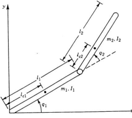
In this project, we design and build a 2-D robot as shown in Figure 1 to test the performance of the proposed algorithm. The actual values of the robot parameters are: m

1

=0.335kg, m

₂

=0.32kg, l

₁

=0.1854m, l

₂

=0.1565m, l

_c1

=0.1m, l

_c2

=0.057m, I

₁

=0.00787531kg-m

²

, and I

2

=0.0020049kg-m

²

. Each joint is coupled to a 30W/24V DC motor with PWM drivers. The joint angles are obtained from a 1024-pulse encoder installed on the motor shaft. An HCTL-2020 chip is used to sample the encoder reading. The angular velocity of each joint is computed using the first-order difference approximation based on the encoder reading. The Advantech PCL-727 AD/DA card is used to interface with a 300MHz Celeron-based computer. The proposed controller and update laws are implemented in a timer ISR under 2ms sampling rate.

Initial condition for the robot arm is q

₁(0)

= q

₂(0)

= q &

₁(0)

= q &

₂(0)

=

0

, i.e., the end-effector is at (0.3149m, 0.0m) initially in the Cartesian space. To have significant nonlinearity, the robot is required to track a 0.08m-radius circle centered at (0.11m, 0.23m) in 1.5 seconds. In this experimental study, D, C and g are assumed to be unknown, and the regressor is unavailable;

therefore, traditional adaptive strategies may not be applied. Let us consider the controller in (18) and update laws in (24), i.e., we ignore the approximation error in the experiment. All elements of D, C and g are approximated by the first 11 terms of the Fourier series. The reason for choosing the Fourier series is its fast convergence property and ease in programming. Hence,

W ~

D

and W ~

_C

are both 44 × 2 matrices and the dimension of W

~_g

is 22 × 2 . Initial weighting vectors of the basis functions are chosen arbitrarily as

1

] 11

0 0

005 . 0 [ ) 0 ˆ ( ) 0 ˆ ( ) 0 ˆ ( ) 0 ˆ ( ) 0 ˆ ( ) 0 ˆ (

22 11

22 21

12 11

ℜ

×

∈

=

=

=

=

=

=

d d d c c ^T

d

w w w w w Λ

w

1

] 11

0 0

0 [ ) 0 ( ˆ ) 0 (

ˆ 11 22

ℜ

×

∈

=

=

c ^T

c

w Λ

w

ˆ (0) ˆ (0) [0.01 0 0] ¹¹¹

2 1

ℜ

×

∈

=

=

g ^T

g

w Λ

w The adaptive gain matrices are selected as

22 ,...

1 , 20 ),

,..., , (

44 ,..., 1 , 10 ),

,..., , (

22 2 1

1

6 44

2 1 1

1

=

∀

=

=

=

∀

=

=

=

−

−

−

i q

q q q diag

i q

q q q diag

gi

g g g

i g

C D

Q Q Q

The controller gains are



 



=



Λ 0 200

0

280 ,





 



=



8 . 6 0

0 8 . 8

K

d

.

Although other values of the initial weightings, adaptive gains and controller gains are also possible to have output error convergence, the above selections give satisfactory performance.

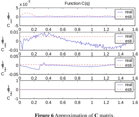
The experimental results are shown in Figure 2 to 7. Figure 2 shows that the end-point trajectory in the Cartesian space converges nicely to the desired trajectory, although the initial position error is quite large. Figure 3 is the joint space tracking performance. It shows that the transient response vanishes within 0.3 seconds. Figure 4 presents the control efforts to the motors. Figure 5 to 7 are function approximation performance. Although estimated parameters do not converge to their true values, they remain bounded as proved in the previous section.

It is worth to note that in designing the controller we do not need much knowledge for the system. All we have to do is to pick some controller parameters and some initial weighting matrices. As for the number of terms of the basis functions, we firstly try an arbitrary number. If the performance is satisfactory, the number is reduced; otherwise, it is increased. Finally, the number can be determined based on the compromise between computation efficiency and tracking performance. Therefore, the proposed controller is very easy to implement.

5. CONCLUSION

We have proposed a function approximation based adaptive controller for a rigid robot

manipulator without using the regressor. The proposed controller does not need to feedback the

joint acceleration, nor does it have to compute the inverse of the estimated inertia matrix.

Analysis of the closed loop stability has been investigated with consideration of the approximation error. For its practical implementation, the control strategy does not require much knowledge about the system model as long as proper sets of basis functions are used.

Experimental results justify its feasibility of giving satisfactory performance on a rigid robot.

REFERENCES

[1] A. Abdallah, D. Dawson, P. Dorato and M. Jamishidi, “Survey of robust control for rigid robots,” IEEE Control System Magazine, vol. 11, no. 2, pp. 24-30, 1991.

[2] D. Cai and Y. Dai, “A globally convergent robust controller for robot manipulator,” Proc.

IEEE Int. Conf. on Control Applications, pp. 328-332, Mexico City, Mexico, 2001.

[3] M. C. Chien and A. C. Huang, “Adaptive impedance control of robot manipulators based on function approximation technique,” accepted by Robotica, 2003.

[4] S. S. Ge, T. H. Lee and C. J. Harris, Adaptive neural network control of robotic manipulators, World Scientific Publishing, Singapore, 1998.

[5] A. C. Huang and Y. S. Kuo, “Sliding control of nonlinear systems containing time-varying uncertainties with unknown bounds,” International Journal of Control, Vol.74, No.3, pp.252-264, 2001.

[6] A. C. Huang and Y. C. Chen, “Adaptive multiple-surface sliding control for single-link flexible-joint robot with mismatched uncertainties,” IEEE Transactions on Control Systems Technology, to appear in the September issue, 2004.

[7] A. C. Huang and Y. C. Chen, “Adaptive multiple-surface sliding control for non-autonomous systems with mismatched uncertainties,” Automatica, to appear in the November issue, 2004.

[8] H. Kawasaki, T. Bito and K. Kanzaki, “An efficient algorithm for the model-based adaptive control of robotic manipulators,” IEEE Trans. on Rob. and Auto., vol. 12, no. 3, pp. 496-501, June 1996.

[9] T. Y. Kuc and W. G. Han, “Adaptive PID learning control of robot manipulators,”

Automatica, vol. 36, no. 5, pp. 717-725, 2000.

[10] W. S. Lu and Q. H. Meng, “Recursive computation of manipulator regressor and its application to adaptive motion control of robots,” IEEE Pacific Rim Conf. on Communication, Computers and Signal Processing, pp. 170-173, May 9-11, 1991.

[11] W. S. Lu and Q. H. Meng, “Regressor formulation of robot dynamics: computation and application,” IEEE Trans. on Robotics and Auto., vol. 9, no. 3, pp. 323-333, Jun. 1993.

[12] Q. H. Meng and Y. Y. Yao, “Design of neural network controller for robots using regressor dynamics,” Proc. IEEE Int. Conf. on Neural Network, pp. 2743-2748, Jun. 27-29, 1994.

[13] M. B. Menhaj and M. Roubani, “A novel neuro-based model reference adaptive control for a two link robot arm,” Proc. IEEE Int. Joint Conf. on Neural Network, pp. 47-52, 2002.

[14] R. Ortega and M. W. Spong, “Adaptive motion control of rigid robots: a tutorial,” Proc. 27

^th

Conf. on Decision and Control, pp. 1575-1584, 1988.

[15] P. R. Pagilla and M. Tomizuka, “An adaptive output feedback controller for robot arms:

stability and experiments,” Automatica, vol. 37, no. 7, pp. 983-995, July 2001.

[16] J. S. Park, Y. A. Jiang, T. Hesketh and D. J. Clements, “Trajectory control of manipulators using adaptive sliding mode control,” Proc. IEEE SOUTHEASTCON, pp. 142-146, 1994.

[17] Z. Qu and J. Dorsey, “Robust tracking control of robots by a linear feedback law,” IEEE Trans. Automatic Control, vol. 36, no. 9, pp. 1081-1084, 1991.

[18] N. Sadegh and R. Horowitz, “Stability and robustness analysis of a class of adaptive controller for robotic manipulators,” Int. J. of Rob. Research, vol. 9, no. 3, pp.74-92, 1990.

[19] E. S. Shin and K. W. Lee, ”Robust output feedback control of robot manipulators using

high-gain observer,” IEEE Int. Conf. on Control Applications, pp. 881-886, 1999.

[20] J.-J. E. Slotine and W. Li, “Adaptive manipulator control: a case study,” IEEE Trans. on Automatic Control, vol. 33, no. 11, pp.995-1003, Nov. 1988.

[21] J.-J. E. Slotine and W. Li, Applied Nonlinear Control, Prentice-Hall, 1991.

[22] Y. D. Song, “Adaptive motion tracking control of robot manipulators: non-regressor based approach,” IEEE Int. Conf. on Robotics and Automation, vol. 4, 00. 3008-3013, 1994.

[23] Y. Stepanenko and J. Yuan, “Robust adaptive control of a class of nonlinear mechanical systems with fast-varying uncertainties,“ Automatica, vol.24, pp.265-276, 1992.

[24] C. Y. Su and Y. Stepanenko, “Adaptive control for constrained robots without using regressor,” Proc. IEEE Int. Conf. on Robotics and Automation, pp. 264-269, 1996.

[25] D. Sun and J. K. Mills,” Performance improvement of industrial robot trajectory tracking using adaptive-learning scheme,” ASME J. of Dynamic System Measurement and Control, vol. 121, no. 2, pp. 285-292, 1999.

[26] D. Del Vecchio, R. Marino and P. Tomei, “Adaptive learning control for robot Manipulators,” Proc. American Control Conference, pp. 641-645, 2001.

[27] J. H. Yang, “Adaptive tracking control for manipulators with only position feedback,” IEEE Canadian Conference on Electrical and Computer Engineering, pp. 1740-1745, 1999.

[28] J. Yim and J. H. Park, “Nonlinear H

_∝

Control of Robotic Manipulator,” IEEE International Conference on Systems, Man, and Cybernetics, vol. 2, pp. 866-871, 1999.

[29] J. Yuan and Y. Stepanenko, “Adaptive PD control of flexible joint robots without using the high-order regressor,” Proc. of the 36

^th

Midwest Symposium on Circuits and Systems, pp.389-393, 1993.

Figure 1 The 2-D rigid robot used in the experiment.

0 0.05 0.1 0.15 0.2 0.25 0.3 0.35 -0.05

0 0.05 0.1 0.15 0.2 0.25 0.3 0.35

X(m) Y(

m )

Cartesian Space Tracking Performance

real desired

Figure 2 Tracking performance of the proposed controller for a 2-D robot in the Cartesian space. Initial position of the end-effector is at the point (0.3149m, 0.0000m). After some transient, the tracking error is very small, although we do not know precise dynamics of the robot.

0 0.2 0.4 0.6 0.8 1 1.2 1.4 1.6 0

1 2 3

q¹ (ra d)

Joint 1 Angle

real desired

0 0.2 0.4 0.6 0.8 1 1.2 1.4 1.6 -0.5

0 0.5 1

Time q²

(ra d)

Joint 2 Angle

real desired

Figure 3 The joint space tracking performance. The first joint converges to the desired

trajectory in 0.4 seconds, while the second joint in 0.1 second.

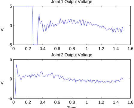
0 0.2 0.4 0.6 0.8 1 1.2 1.4 1.6 -5

0 5

V

Joint 1 Output Voltage

0 0.2 0.4 0.6 0.8 1 1.2 1.4 1.6 -5

0 5

Time V

Joint 2 Output Voltage

Figure 4 Control efforts to the motors. Except for some saturation in the transient stage, the control efforts are reasonable.

0 0.2 0.4 0.6 0.8 1 1.2 1.4 1.6 -0.05

0 0.05

D¹ (q1

)

Function D(q)

real esti

0 0.2 0.4 0.6 0.8 1 1.2 1.4 1.6 -0.01

0 0.01

D¹ (q2

) real

esti

0 0.2 0.4 0.6 0.8 1 1.2 1.4 1.6 -0.01

0 0.01

D² (q1

) real

esti

0 0.2 0.4 0.6 0.8 1 1.2 1.4 1.6 2

4 6x 10^-3

Time D²

(q2

) real

esti

Figure 5 Approximation of D matrix. Although the estimated values do not converge to the

true values, they are bounded and small.

0 0.2 0.4 0.6 0.8 1 1.2 1.4 1.6 -5

0 5x 10^-3

C¹ (q1

)

Function C(q)

real esti

0 0.2 0.4 0.6 0.8 1 1.2 1.4 1.6 -0.01

0 0.01

C¹ (q2

) real

esti

0 0.2 0.4 0.6 0.8 1 1.2 1.4 1.6 -0.05

0 0.05

C² (q1

) real

esti

0 0.2 0.4 0.6 0.8 1 1.2 1.4 1.6 -1

0 1

C² (q2

) real

esti

Figure 6 Approximation of C matrix.

0 0.2 0.4 0.6 0.8 1 1.2 1.4 1.6 -1

0 1 2 3

G1(q)

Function G(q)

real esti

0 0.2 0.4 0.6 0.8 1 1.2 1.4 1.6 -0.1

0 0.1 0.2 0.3

Time G2(q)

real esti

Figure 7 Approximation of vector g.

計畫成果自評

一、與原計畫相符程度

本計畫之研究方法與步驟完全依據原計畫書之規劃而進行，因此其與原計畫完全相符。

二、達成預期目標情況

本計畫達成計畫書中預期之目標。其具體完成之項目計有：

1. Problem formulation

2. Development of the orthonormal function based approximator 3. Development of the adaptive controller

4. Convergence analysis of the closed loop system

5. Analysis of the function approximation error on the system performance

6. Development of a rule for determine the number of basis function for a given function 7. Extensive computer simulation study

8. Design and build a 2-D robot 9. Experimental study

10. Data analysis and performance evaluation 11. Theory refinement

12. Final report preparation

三、研究成果之學術或應用價值

由於本研究所提出之控制器不需要機械臂確切之數學模型、不必計算繁複的迴歸矩 陣、更不需要在各關節安裝加速規，因此不論在學術或工業應用上皆有深遠之貢獻。尤其，

其不但有嚴謹的數學證明來確保所提控制器之理論性能，更有實驗數據以資佐證該理論性 能是可以實現的。在廣泛捜尋各主流期刊歷年處理類似問題之論文後可得到以下結論：本 計畫所提出之控制器所需的假設條件是最少的！並且其性能並不會因為已知條件之減少而 劣化。

四、是否適宜期刊發表或專利申請

本計畫之研究成果極適宜期刊發表。目前已完成初稿撰寫，待完稿後擬投至

SCI

等級

之學術期刊。

可供推廣之研發成果資料表

□ 可申請專利 ▣ 可技術移轉 日期：93 年 8 月 23 日

國科會補助計畫

計畫名稱： 無迴歸矩陣之機械臂適應控制器設計 計畫主持人： 黃安橋

計畫編號：

NSC-92-2212-E-011-018

學門領域： 自動化

技術/創作名稱 無迴歸矩陣之機械臂適應控制器

發明人/創作人 ^黃安橋

中文：本計畫設計出一機械臂之適應控制器，其不需要知道該機械臂之確切模

型。由於此模型中之各矩陣皆為時變且未知其變化邊界，因此傳統的強健控制 或適應控制皆不易直接適用。本計畫中採用函數近似法(FAT)來將這些未知量表 示成有限項正交級數之線性組合，進而可以將輸出追蹤動態行為表示成一由近 似誤差所驅動之一階線性穩定濾波器。藉由 Lyapunov 理論可證得閉迴路系統之 穩定度，同時可一併求得相關之適應率。本計畫中設計且實作出一具 2-D 機械 臂以測試所提控制器之性能。實驗結果顯示其可在未知系統參數之情況下，迅 速使機械臂收斂至期望軌跡。

技術說明 ^英文： An adaptive control scheme is proposed for an n-link rigid robot manipulator without using the regressor. The robot is firstly modeled as a set of second-order nonlinear differential equations with the assumption that all of the matrices in that model are unavailable. Since these matrices are time-varying and their variation bounds are not given, traditional adaptive or robust designs do not apply. The function approximation technique (FAT) is used here to represent uncertainties in some finite linear combinations of the orthonormal basis. The dynamics of the output tracking can thus be proved to be a stable first order filter driven by function approximation errors. Using the Lyapunov stability theory, a set of update laws is derived to give closed loop stability with proper tracking performance. A 2-D robot is built in this project to test the efficacy of the proposed scheme. Experimental results confirm that it can give satisfactory performance.

可利用之產業 及 可開發之產品

可利用之產業：工業機器人相關產業 可開發之產品：工業機器人控制器

技術特點

1. 控制器設計時無需知道機械臂之數學模型 2. 無需各關節之加速度回授

3. 無需計算迴歸矩陣

4. 系統穩定度具有嚴謹之數學證明與實驗驗證

推廣及運用的價值

1. 使機械臂控制器之設計更為容易 2. 節省加速度規與相關處理電路之成本

3. 提升機械臂運動控制之性能