A new maximal-margin spherical-structured multi-class support vector machine

A New Maximal-Margin Spherical-Structured Multi-class Support

Vector Machine

Pei-Yi Hao*

Department of Information Management

National Kaohsiung University of Applied Sciences, Kaohsiung, Taiwan

haupy@cc.kuas.edu.tw

Jung-Hsien Chiang

Department of Computer Science and Information Engineering National Cheng Kung University, Tainan, Taiwan

jchiang@mail.ncku.edu.tw

Yen-Hsiu Lin,

Department of Computer Science and Information Engineering National Cheng Kung University, Tainan, Taiwan

yanxiu@cad.csie.ncku.edu.tw

Following is the address for correspondence:

Prof. Pei-Yi Hao

Department of Information Management

National Kaohsiung University of Applied Sciences, Kaohsiung, Taiwan e-mail: haupy@cc.kuas.edu.tw

Tel: 886-7-3814526-6112 Fax: 886-7-3831332

______________________________________________ * author to whom correspondence should be addressed.

Abstract

Support vector machines (SVMs), initially proposed for two-class classification

problems, have been very successful in pattern recognition problems. For multi-class

classification problems, the standard hyperplane-based SVMs are made by

constructing and combining several maximal-margin hyperplanes, and each class of

data is confined into a certain area constructed by those hyperplanes. Instead of using

hyperplanes, hyperspheres that tightly enclosed the data of each class can be used.

Since the class-specific hyperspheres are constructed for each class separately, the

spherical-structured SVMs can be used to deal with the multi-class classification

problem easily. In addition, the center and radius of the class-specific hypersphere

characterize the distribution of examples from that class, and may be useful for

dealing with imbalance problems. In this paper, we incorporate the concept of

maximal margin into the spherical-structured SVMs. Besides, the proposed approach

has advantage of using a new parameter on controlling the number of support vectors.

Experimental results show that the proposed method performs well on both artificial

and benchmark datasets.

Keywords: support vector machines (SVMs), multi-class classification, spherical

1. Introduction

The support vector machine (SVM) is a very promising machine learning

method proposed by Vapnik et al. [Cortes, 1995; Vapnik, 1998]. Based on the idea of

VC-dimension and the principal of structural risk minimization, an SVM is intuitively

a two-class classifier in the form of a hyperplane that leaves the largest possible

fraction of points of the same class on the same side, while maximizing the distance

of either class from the hyperplane. The optimal maximal-margin hyperplane

minimizes not only the empirical risk, but also the upper bound on the expected risk,

and thus has better generalization ability compared with traditional classifiers.

Because of their excellent performance and simple structures, SVMs have been

applied to many fields. Although SVMs were initially proposed for two-class

classification problems, two main approaches have been proposed to solve multi-class

classification problems currently [Hsu, 2002]. One is all-together multi-class SVM

that directly considers all classes in one optimization formulation [Weston, 1999;

Crammer, 2000], while the other is combined multi-class SVM that constructs several

binary classifiers through methods such as one-against-all [Bottou, 1994],

one-against-one [Kreel, 1999], directed acyclic graph SVM (DAG-SVM) [Platt, 2000]. All these SVM classifiers belong to algorithms based on a maximal-margin

hyperplane. To a multi-class problem, such SVMs are to divide the data space by

several hyperplanes and each class of data is confined into a certain area constructed

by a number of hyperplanes.

Instead of using a hyperplane, a hypersphere around the examples of one class

can be used. Given a set of training data, the minimum bounding hypersphere is

defined as the smallest hypersphere that encloses all the data. The minimum bounding

hypersphere was first used by Schölkopf, Burges, and Vapnik to estimate the

to data domain description [Tax, 1999; 2004]. In [Schölkopf, 2001], Schölkopf et al. proposed a hyperplane-based one-class SVM and showed that it is equivalent to the minimum bounding hypersphere when using the Gaussian RBF kernel. Inspired by the minimum bounding hypersphere, spherical-structured SVMs have been proposed

to solve the multi-class classification problems [Manevitz, 2001; Wu, 2005; Zhu,

2003]. The same class of data being bound by an optimal class-specific hypersphere,

the whole data space is then divided by a number of such hyperspheres. Experimental

results have showed that the spherical-structured SVMs perform comparable to the

standard hyperplane-based SVMs [Manevitz, 2001; Wang, 2005; Wu, 2005; Zhu,

2003].

Motivated by the Bayes decision theory, an optimal classifier should consider

the probability distribution, including the mean and variance, of each class. The use of classical hyperplane-based SVM for probability density estimation was first introduced in [Mukherjee, 1999]. Schölkopf et al. also showed that the hyperplane-based one-class SVM [Schölkopf, 2001] can be used as a probability density estimator. In contrast to the hyperplane-based SVMs, the hypersphere-based SVMs provide the information of spherical center and radius, which characterize the probability distribution for each class more intuitive, and may be useful for dealing with class-imbalance problems. In this paper, inspired by the maximal-margin SVM classifier and the spherical-structured SVMs, we propose a novel maximal-margin

spherical-structured multi-class support vector machine (MSM-SVM). The

MSM-SVM finds several class-specific hyperspheres that each encloses all examples

from one class but excludes all examples from the rest class. In addition, the

hypersphere separates those classes with maximal margin. Moreover, the proposed

approach has advantage of using a new parameter on controlling the number of

The rest of this paper is organized as follows. First, we give a brief overview of

the spherical-structured SVMs. In section 3 we address the proposed maximal-margin

spherical-structured multi-class SVM, and then analyze its properties theoretically in

2. Previous Works

Spherical classifiers [Wang, 2005] were first introduced into pattern

classification by Cooper in 1962 [Cooper, 1962; 1966]. One well-known

classification algorithm consisting of spheres is the Restricted Coulomb Energy (RCE)

network [Reilly, 1982]. The RCE network is a supervised learning algorithm that

learns pattern categories by representing each class as a set of prototype regions -

usually spheres. Another well-known spherical classifiers is the set covering machine

(SCM) proposed by Marchand and Shawe-Taylor [Marchand, 2002]. In their

approach, the final classifier is a conjunction or disjunction of a set of spherical

classifiers, where every spherical classifier dichotomizes the whole input space into

two different classes with a sphere.

Spherical classification algorithms [Wang, 2005] normally need a number of

spheres in order to achieve good classification performance, and therefore have to

deal with difficult theoretical and practical issues such as how many spheres are

needed and how to determine the centers and radius of the spheres. In contrast to

previous spherical classifiers that construct spheres in the input space, the basic idea

of the spherical-structured SVMs [Manevitz, 2001; Wang, 2005; Wu, 2005; Zhu,

2003] is to construct class-specific hyperspheres in the feature space induced by the

kernel.

2.1 Support Vector Domain Description (SVDD)

Tax and Duin introduced the use of a data domain description method [Tax,

1999; 2004], inspired by the SVM developed by Vapnik. Their approach is known as

the support vector domain description (SVDD). In domain description the task is to

give a description of a set of objects. This description should cover the class of

objects represented by the training set, and should ideally reject all other possible

(a)

(b)

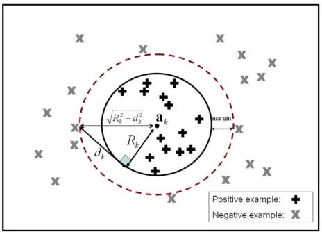
Figure 1. Support vector domain description.

We now illustrate the support vector domain description method as shown in

Figure 1. To begin, let  denotes a nonlinear transformation, which maps the original input space into a high-dimensional feature space. Data domain description

gives a closed boundary around the data: a hypersphere. As shown in Figure 1 (a) the

SVDD may be viewed as finding a smallest sphere, which is characterized by its

center a and radius R, that encloses all the data points in the feature space. The

contour diagram shown in Figure 1 (b) can be obtained by estimating the distance

between the spherical center and the corresponding input point in the feature space.

The larger the distance, the darker is the gray level in the contour diagram. The

algorithm then further identifies domain description using the data points enclosed

inside the boundary curve. The mathematical formulation of the SVDD is as follows.

Given a set of input patterns,{x_i}_i1,...,N, the support vector domain description method is to find

, 0 , ) ( subject to minimize 2 2 2 a, , i R C R i i i i i ξ R i      



    a x (2.1)

where R is the radius and a is the center of the enclosing hypersphere;



_i is a slack variable; and C is a constant controlling the penalty of noise. Using the Lagrangian

theorem, we can formulate the Wolfe dual problem as





    j i j i j i i i i i L i _, ) ( ) ( ) ( ) ( maximize  x  x    x  x  (2.2) subject to



_1 i i  and 0iC  i,

where {_i}_i1,...,N are the Lagrange multipliers and  denotes the inner product. Solving the dual quadratic programming problem gives the Lagrange multipliers _i for all i. The center a and the radius R can be subsequently determined by





i

i

i (x )

a   and R (x_i)a i such that 0_i C.

In real-world applications, training data of a class is rarely distributed spherically

[Wang, 2005]. To have more flexible descriptions of a class, one can first transform

the training examples into a high-dimensional feature space by using a nonlinear

mapping  and then compute the minimum bounding hypersphere in that feature space. For certain nonlinear mappings, there exists a highly effective method, known

as the kernel trick, for computing inner products in the feature space. A key property

of the SVMs is that the only quantities that one needs to compute are inner products,

of the form (x)(y) . It is therefore convenient to introduce the so-called kernel function K(x,y) (x)(y) . The functional form of mapping (x) does not need to be known since it is implicitly defined by the choice of kernel function. The

) ( ) (x  y

  with a kernel functionK( yx, ), the resulting hypersphere may actually

represent a highly complex shape in the original input space, as illustrated in Figure 1.

2.2 Support Vector Domain Description for Multi-Class Problem (M-SVDD)

Inspired by the support vector domain description, spherical-structured SVMs

have been proposed to solve the multi-class classification problems [Manevitz, 2001;

Wu, 2005; Zhu, 2003]. Given a set of training data (x₁,y₁),...,(x_N,y_N), where

n iR

x and y_i{1,...,K} is the class of x , the minimum bounding hypersphere _i

of each class is the smallest hypersphere enclosing all the training examples of that

class. The minimum bounding hypersphere S for each class k, which is _k

characterized by its center a and radius _k R , can be found by solving the following _k

constrained quadratic optimization problem:



  k y i i k k R i i k k N C R : 2 , , minimize   a (2.3a)

subject to (x_i)a_k 2 R_k2 _i i such that y_i k, (2.3b) ,

0 i

i  

 (2.3c) where  are slack variables, C>0 is a constant that controls the penalty to errors, _i and N is the number of examples within class k. Using the Lagrange multiplier _k method, this quadratic programming problem can be formulated as the following

Wolfe dual form:





  k _{iy k} i i i _{i jy y k}i j i j y j i i i i K K , : , : : ( , ) ( , ) maximize  x x  x x  (2.4a) subject to 1 : 



k y i i i  , (2.4b) k y i N C i k i     such that 0  . (2.4c)

Figure2. A comparison of hyperplane-based SVMs and hypersphere-based SVMs in decision boundary.

After all K class-specific hyperspheres are constructed, we can determine the

membership degree of a data point x belonging to class k based on the center a and _k

radius R of the class-specific hypersphere _k S . By using a similarity function _k )

, ( S_k

sim x , we say x is in the class that has the largest value of the similarity

function:

class of arg max ( , )

1 K k k sim x S x    .

Imbalanced data distribution is a familiar phenomenon in classification problems.

For instance, Figure 2 indicates two classes of examples generated from the Gaussian

distribution with different variance and number of data. In some iterative

update-based learning machines (such as back-propagation neural networks) the final

decision function is deviated to the class with smaller number of data points due to it

takes more back-propagation update iterations in the class with larger number of data

points. The hyperplane-based SVMs classifier does not suffer this bias. The

hyperplane-based SVMs construct a hyperplane that leaves the largest possible

fraction of points of the same class on the same side, while maximizing the distance

of either class from the hyperplane, and the distance is called margin, as shown in

of boundaries of each class, but not the information of distribution, for instance the

mean and variance, of each class. According to the Bayesian decision rule, the

optimal decision function is defined as minimizing the error probability [Fukunaga,

1990] and with location slightly deviated to the class with smaller variance. In

Contrast to hyperplane-based SVM, the hypersphere-based SVM takes the

distribution for each class into account. Therefore, taking into consideration the

spherical center (mean) and the spherical radius (variance) in the feature space, the

hypersphere-based SVM resembles more the optimal Bayesian classifier.

2.3 Support Vector Domain Description with Negative Examples for Multi-Class Problem (M-SVDD-NEG)

Given the fact that a minimum bounding hypersphere of each class is constructed

without considering the distribution of training examples of other classes, it is not

immediately clear whether or not an effective classifier can be built based on these

class-specific minimum bounding hyperspheres. Tax et al. proposed a new algorithm

to incorporate the negative examples in the training phase to improve the description

[Tax, 2004]. In contrast with the positive examples (examples in the kth class), which

should be within the class-specific hypersphere S , the negative examples (all other _k examples) should be outside it. The minimum bounding hypersphere S for each _k class k can be found by solving the following constrained quadratic optimization

problem:





    k y l l k k y i i k k R l i l i k k N C N C R : : 2 , , , minimize     a (2.5a)

subject to (x_i)a_k 2 R_k2_i i such that y_i k, (2.5b) k y l R_{k l l} k l)    such that  ( 2 2   x a , (2.5c) l i l i 0, 0 ,  (2.5d)

where  , _i  are slack variables. _l N and _k N are the number of examples within _k the kth class and the rest class, respectively. Using the Lagrange multiplier method,

this quadratic programming problem can be formulated as the following Wolfe dual

form:           











      k y y m l l m l m k y l k y i i l i l k y y j i j i j i k y l l l l k y i i i i m l l i j i l i K K K K K , : , : , : , : , : : ) , ( ) , ( 2 ) , ( ) , ( ) , ( maximize x x x x x x x x x x         (2.6a) subject to 1 : :  





  ly k l k y i i l i   , (2.6b) k y i N C i k i     such that 0  , (2.6c) k y l N C l k l     such that 0  . (2.6d)

Solving the dual quadratic programming problem gives the Lagrange multipliers _i and _l. The center a and the radius _k R of the class-specific hypersphere _k S _k

can be subsequently determined by





    k y l l l k y i i i k l i : : ) ( ) (x x a   , (2.7) k i k

R  (x )a i such that y_i  and k

k

i  _NC



3. Methodology

Inspired by the maximal-margin hyperplane-based SVM and the support vector domain description (SVDD), Wang et al. [Wang, 2005] first incorporated the concept of maximal-margin into hypersphere-based SVM for two-class classification problem via a single sphere. In this section, we propose a modification of the Wang’s approach, called the maximal-margin spherical-structured multi-class support vector machine (MSM-SVM). The MSM-SVM finds several class-specific hyperspheres that each encloses all examples from one class but excludes all examples from the rest class. In

addition, the hypersphere separates the positive examples from the negative examples

with maximal margin.

3.1 The Quadratic Programming Problem

Given a set of training data (x₁,y₁),...,(x_N,y_N), where y_i{1,...,K} is the class of x_i, we first map training points into a high-dimensional feature space via a nonlinear transform , and then find K class-specific hyperspheres with minimal radius in the feature space such that the kth hypersphere encloses all data points

within the kth class (positive examples) but excludes all examples from the rest class

(negative examples). In addition, according to the concept of maximal margin, the

negative examples shall far away from the kth hypersphere. As illustrated in Figure 3,

the margin is defined as the distance from the nearest negative example to the

boundary of hypersphere. Maximizing the margin will lead the negative examples far

away from that hypersphere. By introducing a new margin factor, d , the _k

MSM-SVM is derived to separate the positive examples from the negative examples

with maximal margin. Mathematically, the class-specific hypersphere S for each _k class k, which is characterized by its center a_k and radius R , can be found by _k solving the following constrained quadratic optimization problem:

Figure 3. Spherical structured SVM that maximizes the margin. QP3.1





     k y l l k k y i i k k k d R l i l i k k k N C N C Md R : : 2 2 , , , , minimize     a (3.1a)

subject to (x_i)a_k 2 R_k2_i i such that y_i k, (3.1b) k y l d R_{k k l l} k l)     such that  ( 2 2 2   x a , (3.1c) 0 , 0   _l i    (3.1d) i,l where N and _k N are the number of examples within the kth class and the rest _k class, respectively. The positive examples are enumerated by indices i, j and the

negative examples by l, m. _i and _l are slack variables and parameter C0 controls the penalty to errors. Figure 3 gives a geometrical point of view explaining the relationship between the margin factor d_k and the width of margin. As shown in Figure 3, the width of margin in our approach is R_k2d_k2 R_k

. To maximize the

margin, we need to maximize d_k2 and minimize R_k2 simultaneously, and the parameter M 0 controls the trade-off between those two terms. We can find the

solution to this optimization problem in dual variables by finding the saddle point of the Lagrangian:









_

_









               l l l i i i l l k k k l l i k i i k i l l k i i k k k l i l i l i k k k d R R N C N C Md R d R L                   2 2 2 2 2 2 2 ) ( ) ( ) , , , , , , , , ( a x a x a

where _i, _l, _i, and _l are nonnegative Lagrange multipliers. Differentiating L with respect to d , _k R , _k a , _k _i, and _l and setting the result to zero, we obtain:

0 2 2      

_

l l k k k d M d d L _{  M} l l 



 (3.2) 0 2 2 2      

_

_

l l k i i k k k R R R R L _{  }

_

_

_

_1 l l i i   (3.3) 0 2 ) ( 2 2 ) ( 2                    









l l k l l l i i k i i i k L       a x a x a  







l l l i i i k (x ) (x ) a     (3.4) 0       i i k i N C L _{ }   k i i k i N C N C _{ }     and (3.5) 0       l l k l N C L _{ }   k l l k l N C N C _{ }     and . (3.6)

Substituting Eqs. (3.2)-(3.6) into L, we obtain the following dual form of the

quadratic programming problem:

QP3.2           











m l m l m l l i l i l i j i j i j i l l l l i i i i K K K K K , , , ) , ( ) , ( 2 ) , ( ) , ( ) , ( maximize x x x x x x x x x x         (3.7a) subject to M i i  



 1 , (3.7b) M l l 



 , (3.7c)

k i  _NC  0  such that i y_i k, (3.7d) k l  _NC 

0  such that l y_l k, (3.7e) where K(x,y) (x)(y) is the kernel function. Solving the dual quadratic

programming problem QP3.2, we obtain the Lagrange multipliers _i and _l , which give the spherical center a_k as a linear combination of (x_i) and (x_l):





  l l l i i i k (x ) (x ) a    . (3.8)

We can determine the distance from a data point (x) to the center a of the kth _k

hypersphere by the following equation

. ) , ( ) , ( 2 ) , ( ) , ( 2 ) , ( 2 ) , ( ) ( , , , 2











       m l m l m l l i l i l i j i j i j i l l l i i i k K K K K K K x x x x x x x x x x x x a x          (3.9)

Knowing a_k, we can subsequently determine the spherical radius R_k and the margin factor d_k of the kth hypersphere by exploiting the Karush-Kuhn-Tucker (KKT) conditions:



_k2  _i  ( _i) _k 2



0 i R   x a  , (3.10)



( _l) _k 2  _k2  _k2  _l



0 l  R d   x a , (3.11) 0         _{i i} k N C _{ } , (3.12) 0           _{l l} k N C _{ } . (3.13)

For some _i(0,C N_k)and _l (0,C N_k), we have _i _l 0 (using Eqs. (3.12) and (3.13)) and moreover the second factor in Eqs. (3.10) and (3.11) has to vanish. Hence, we can subsequently determine the spherical radius R_k and the

margin factor d_k by setting 2 2 ) ( _{i k} k a R   x  i such that k i N C   0 , (3.14) 2 2 2 ) ( _{l k k} k a R d   x   l such that k l N C   0 . (3.15)

3.2 The Decision Rule

Given a collection of training example



(x₁,y₁),...,(x_N,y_N)



and }

,..., 1

{ K

y_i , K class-specific hypersphere S can be constructed by solving the _k QP3.2 for each class. For classifying a new test example x, we can use the following

decision rule:

class of arg max ( , )

1 K k k sim x S x    , (3.16)

where )sim x( ,S_k is the similarity function which determines the membership degree of the test example x belonging to the hypersphere S . We say x is in the class that _k has the largest value of the similarity function. In this Section, we present several

similarity functions that have been proposed in previous spherical-structured SVM

classifiers. A comparison of those similarity functions in classification performance

will be given in the experimental part.

a. Distance-to-Center-based Similarity Function

The simplest similarity function is

2 ) ( ) , ( S_{k k} sim x  x a , (3.17) which calculates the distance from (x) to the center a of the kth hypersphere. _k

The value of sim x( ,S_k) is higher as (x) is closer to a . _k

Zhu et al. proposed a method for classifying a new test example x based on

the following similarity function

2 2 ) ( ) , ( S_k R_{k k} sim x    x a . (3.18) This similarity function considers not only the distance between (x) and a , but _k

also the spherical radius R . _k

c. Gaussian-based Similarity Function

Suppose that the training examples from class k are generated from the

Gaussian distribution in the high-dimensional feature space with mean a and _k

variance R , respectively. Then, according to the Bayesian decision rule, we can use _k2 the following similarity function

       _{ }  2 2 ) ( exp 1 ) , ( k k k k R R S sim x  x a . (3.19)

d. Wu’s Similarity Function [Wu, 2005]

Let the number of hyperspheres that contain the new test example x be d. Wu et al. [Wu, 2005] proposed the similarity functions which involved the following cases:

Case 1: d=0.

If the test point is precluded by all the hyperspheres, seek the nearest one

to x, i.e., k k k R S sim(x, )  (x)a . (3.20) Case 2: d=1.

If the test point x is included in only one hypersphere, it belongs to the

corresponding class.

If the test point x is located in the common area of a number of

hyperspheres, the output class can be obtained by comparing the distance

between the test point and the center of each hypersphere. To eliminate

the effect of different spherical radius, a relative distance is applied, i.e.,

k k k R S sim(x, ) (x)a . (3.21)

e. Chiang’s Similarity Function [Chiang, 2003]

In our previous work [Chiang, 2003], we proposed the following fuzzy

membership function to determine the membership degree of a new test example x

belonging to each hypersphere in the feature space.





                                                         otherwise , ) ( 1 1 5 . 0 ) ( if , 5 . 0 ) ( 1 1 ) ( 1 1 5 . 0 ) , ( 2 1 k k k k k k k k k R R R R S sim a x a x a x a x x       (3.22)

where₁ and ₂ are user predefined parameters; and the parameters ₁ and ₂ satisfy ) 1 ( 1 1 2 _    k R ,

which makes sim x( ,S_k) differentiable as (x) a_k R_k.

Some important properties of the proposed similarity function are summarized

as follows. The greater the distance between the new test point and the spherical

center, the lower the degree of membership of the point belonging to that class is.

Moreover, the membership value also takes into account the radius of the

corresponding hypersphere in the feature space. The overall membership functions

can be seen that the membership value remains higher than 0.5 if the new test

example is located inside the hypersphere in the feature space and smaller than 0.5

otherwise. In the following experiments, we set  =0 and 1

k

R 1

2 

4. The Properties

Comparing the proposed MSM-SVM with M-SVDD and M-SVDD-NEG, the

M-SVDD considers only the positive examples; while the M-SVDD-NEG

incorporates both the positive and negative examples to improve the classification

performance. In contrast to M-SVDD and M-SVDD-NEG, the proposed MSM-SVM

finds several hyperspheres that each separates the positive examples from the

negative examples with maximal margin by introducing a new margin parameter M.

In this section, we analyze our approach theoretically. Besides, we discuss the

significance of the margin parameter M.

4.1 The Feasible Range

The quadratic programming problem QP3.2 is not feasible for any pair of (C,M).

First, we discuss the feasible range of the margin parameter M. From Eqs. (3.7b) and

(3.7d), we have C M    1 0 . (4.1)

Similarly, from Eqs. (3.7c) and (3.7e), we have C

M  

0 . (4.2)

From the above two inequalities, we obtain the following result

1

0M C . (4.3) Therefore, QP3.2 has feasible solution when we set C1 given that M is in the range of [0, C-1].

4.2 The Bound on Number of Support Vectors

Solving the dual quadratic programming problem given in QP3.2, we obtain the Lagrange multipliers _i and _l. The Karush-Kuhn-Tucker conditions (see Eqs. (3.10)-(3.13)) make several useful conclusions to us. The training point x_i for which

i

 (_l)>0 are termed support vectors (SVs) since only those points are relevant to the final hypersphere among all training points. Here we have to distinguish the difference between the examples for which 0_i C N_k (or 0_l C N_k ),

and those for which _i C N_k (or _l C N_k ). In the first case, from Karush-Kuhn-Tucker (KKT) conditions (3.12) (or (3.13)), it follows _i _l 0 and moreover the second factor in Eq. (3.10) (or Eq. (3.11)) has to vanish. In the second case, according to the Karush-Kuhn-Tucker (KKT) conditions (see Eqs. (3.12)-(3.13)), we have k i  _NC   (x_i) a_k 2 R_k2 and _i 0, (4.4) k l  _NC   (x_l) a_k 2 R_k2 d_k2 and _l 0. (4.5)

Here, we will use the term outlier support vector (OSV) to refer to the training points for which k i N C   (or k l N C   ).

The number of the support vectors (SVs) influences the time complexity in the testing phase. More importantly, the number of the support vectors is related to the generalization ability of the resulted SVM classifier. Now, let us analyze the theoretical aspects of the new optimization problem given in QP 3.2. The following proposition explains the bound on the number of the support vectors (SVs) and outlier support vectors (OSVs) in the proposed MSM-SVM algorithm.

Proposition. Suppose QP3.2 leads to the class-specific hypersphere S for a given _k

(C,M). The following results hold:

i. The upper bound on number of OSVs from the positive examples is

C N

M 1) k

( 

.

ii. The upper bound on number of OSVs from the negative examples is C

MN_k

iii. The lower bound on number of SVs from the positive examples is C N M 1) k (  .

iv. The lower bound on number of SVs from the negative examples is

C MN_k

.

Proof:

(i). The constraints, Eqs. (3.7b) and (3.7d), imply that at most

C N

M 1) _k

( 

of all

positive training examples can have

k i

N C



 . All positive examples with _i 0 certainly satisfy k i N C 

 (if not, _i could grow further to reduce _i).

(ii). The constraints, Eqs. (3.7c) and (3.7e), imply that at most

C MN_k

of all negative

training examples can have

k

l _N

C



 . All negative examples with _l 0

certainly satisfy

k l _N

C



 (if not, _l could grow further to reduce _l).

(iii). Since support vectors are those examples for which _i 0. The constraints, Eqs. (3.7b) and (3.7d), imply that at least

C N

M 1) k

( 

of all positive training

examples can have _i 0.

(iv). Since support vectors are those examples for which _l 0. The constraints, Eqs. (3.7c) and (3.7e), imply that at least

C MN_k

of all negative training examples can

have 0_l  .

Let us denote by SV ,_k OSV the number of support vectors (SVs) and outlier _k support vectors (OSVs) in the kth class-specific hypersphere S , respectively. The _k following results are a consequence of the above proposition:

             C MN C N M SV k k k ) 1 ( , (4.6)

             C MN C N M OSV k k k ) 1 ( . (4.7)

Hence, parameters C and M can be used to control the number of support vectors and

outlier support vectors. Note that all outlier support vectors (OSVs) are also support vectors (SVs), but there can be SVs which are not OSVs. Hence, SV_k OSV_k in the

kth class-specific hypersphere S_k.

We now discuss the generalization ability of the proposed MSM-SVM

algorithm. Since removing a non-support vector from the training set does not change

the optimal solution obtained by QP3.2. When one of the non-support vectors is left

out in the training phase, during testing this vector will therefore be classified

correctly, which gives the following bound on the number of errors made by the

leave-one-out (LOO) error estimate procedure [Vapnik, 1998]:



 k k LOO N SV E~ . (4.8)

4.3 The IRIS Example

Before we give an example to illustrate the influence of the margin parameter M,

we discuss a special case on the choice of parameters C and M. As 1

C M , we have N N N C MN C N M SV N k k _{k k} k                 ( 1) _{, (4.9)}

which indicates that almost all training examples turn into the support vectors as we

(a) (b)

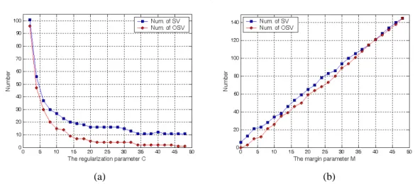
Figure 4. (a) The number of SVs and OSVs vs. regularization parameter C, and (b) the number of SV and OSV vs. margin parameter M.

Now, we use the Iris data [Blake, 1998] to characterize the dependence of SV _k and OSV on the parameters C and M. The Iris flowers data set consists of three _k classes: setosa, versicolor, and virginica; where 150 instances are available, 50 for

each class. Each instance has four attributes: septal length, septal width, petal length,

and petal width. In this example, we set setosa as the positive class and the remaining

as the negative class. In addition, we used the Gaussian RBF kernel

) exp(

) ,

(x y   xy 2

K with kernel parameter  1.

Figure 4(a) illustrates the number of support vectors and outlier support vectors

of the resulted MSM-SVM with M=1 and varying value of C. As shown in Figure

4(a), when M is fixed, SV and _k OSV is decreased as C increases. Figure 4(b) _k illustrates the number of support vectors and outlier support vectors of the resulted

MSM-SVM with C=50 and varying value of M. As shown in Figure 4(b), when C is fixed, SV and _k OSV is increased as M increases._k

5. Experiments

We present two types of experiments to demonstrate the performance of the

proposed MSM-SVM algorithm. First, we present a 2D artificial dataset that can be

visualized in the plane. We then apply the proposed method to benchmark datasets.

We solve the optimization problem QP3.2 based on the Sequential Minimal

Optimization (SMO) algorithm [Fan, 2005; Platt, 1999]. The optimization problems

of one-against-all, one-against-one and DAGSVM are implemented by LIBSVM 2.17

[Chang, 2001]. For each problem we stop the optimization algorithm if the KKT

violation is less than 104. Throughout this experimental part we used Gaussian RBF

kernel K(x,y)exp( xy 2) for all algorithms. In the following experiments, when we used Chiang’s fuzzy similarity function mentioned in Section 3.2, we simply

set 1=0 and k R 1 2   . 5.1 Artificial Dataset

To demonstrate that the hypersphere-based multi-class SVM can be useful for

dealing with imbalance problem than hyperplane-based multi-class SVM, we first

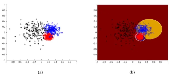
give an artificial dataset. As shown in Figure 5(a), we draw randomly three classes of

examples from the Gaussian distribution where their class distribution means are

[-0.2, –0.05]t, [0.3, 0.1]t, and [0.2, -0.15]t with standard-deviations() 0.2, 0.1, and 0.05, respectively. Figure 5(b) illustrates the optimal decision boundary obtained by

the Bayes decision rule according to the true probability density function of each

class. We compare the proposed MSM-SVM approach with three different types of

hyperplane-based multi-class SVMs, including one-against-all [Bottou, 1994],

(a) (b)

Figure 5. (a) The artificial imbalance dataset where 600 examples are available, 200 for each class (testing samples bold face), and (b) the optimal decision boundary obtained by the Bayes decision rule.

Note that the generalization errors of the classifier depend on the values of the

kernel parameter  and the regularization parameter C. However, it is unfair to use only one parameter set for comparing these methods. In this experiment, we separate

the dataset into three disjoint subsets: the training set (40%) is used to learn the

classifier; the validation set (20%) is used to select the model parameters; and the test

set (40%) is used to obtain an unbiased estimate of error. According to their validation

error, we try to infer the proper values of model parameters. If several (C, ) have the same accuracy in the validation stage, we report the parameter set with least errors in

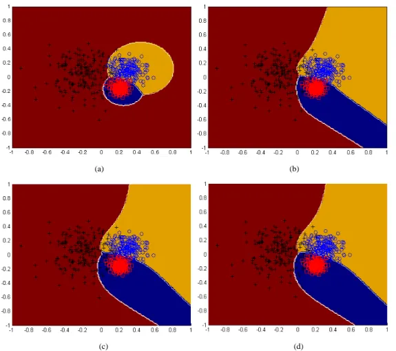
the training stage. Figure 6(a) shows the decision boundary obtained by our approach

using the Chiang’s similarity function. Figures 6 (b), (c) and (d) show the decision

boundary obtained by the one-against-all method, one-against-one method, and

DAGSVM, respectively. As can be seen, our approach resembles more the optimal

Bayesian classifier. Table I presents the result of comparing these methods. We report

(a) (b)

(c) (d)

Figure 6. The decision boundaries obtained by (a) the proposed MSM-SVM approach, (b) one-against-all method, (c) one-against-one method, and (d) DAGSVM approach.

Table I. A comparison of classification performance

Algorithm Model parameters Num. of misclassified patterns

Training set Validation set Test set

Proposed MSM-SVM C=10, =2, M=0.5 17 4 14

One-against-all SVM C=20, =32 18 6 21

One-against-one SVM C=40, =14 21 8 24

DAGSVM C=40, =14 21 8 24

As shown in Figure 6, the misclassified patterns in the hyperplane-based SVM

are belonged to the larger variance and sparser class. The proposed algorithm

achieves better generalization ability in this artificial dataset, which demonstrates that

the spherical-structured SVMs are more suitable for the imbalance problem as it deals

with the distribution, characterized by the spherical center and radius, of each class.

Here we should note that the radius of the hypersphere for each class in the feature

the feature space is nearly proportional to the standard-deviation () of the three classes in the original space. It demonstrates that we can use the radius of the

hypersphere in the feature space to characterize the class distribution variance in the

original space.

5.2 Benchmark Datasets

In this section we present experimental results on several benchmark datasets.

From UCI Repository [Blake, 1998] we choose the following datasets: iris, wine, dermatology, house-vote-88, ionosphere, and sonar. From Statolog Collection [Michie, 1994] we choose following datasets: vehicle and german. Furthermore, we

choose face and imox from [Mitchell, 1997] and [Chen, 2005], respectively. In this

experiment, we compare our approach with the hyperplane-based multi-class SVMs

approaches, including one-against-all, one-against-one, and DAGSVM. Besides, we

compare our approach with the hypersphere-based multi-class SVMs, including

M-SVDD and M-SVDD-NEG. For hypersphere-based SVMs, we evaluate the

classification performance by using different similarity functions mentioned in

Section 3.2.

The most important criterion for evaluating the performance of those methods is

their accuracy rate. However, it is unfair to use only one parameter set for comparing

these methods. Practically for any method, the best parameters are first obtained by

performing model selection. For each problem, we estimate the generalized accuracy

using different kernel parameters  = [22,21,20,…,2-15] and regularization parameter C = [215

,212,211,…,2-4]. Therefore, for each problem we try 1820 combinations [Hsu, 2002]. We apply the five-fold cross-validation method to select the model parameters. Namely, for each problem we partition the available examples into five disjoint

subsets except for one, and the validation error is measured by testing it on the subset

left out. This procedure is repeated for a total of five trails, each time using a different

subset for validation. The performance of the model is assessed by averaging the

squared error under validation over all the trails of this problem. According to their

cross-validation rate, we try to infer the proper values of model-parameters.

Table II. A comparison of classification performance (best rates bold faced)

iris wine dermat-ology

house-vote-88

ionosph-ere sonar vehicle german face imox one-againat-all (C,) 98.000 (5,-3) 97.837 (4,-2) 97.297 (15,-11) 97.021 (4,-6) 95.211 (1,-3) 66.976 (7,-7) 84.795 (9,-4) 75.500 (3,-3) 98.970 (11,-15) 93.000 (1,-1) one-against-one (C,) 98.000 (1,-1) 98.918 (4,-1) 98.108 (11,-9) 97.021 (5,-7) 95.211 (2,-4) 66.976 (7,-7) 85.029 (10,-4) 75.500 (3,-3) 98.823 (9,-14) 93.500 (2,0) DAGSVM (C,) 98.000 (1,-1) 98.918 (4,-1) 98.108 (14,-10) 97.021 (5,-7) 95.211 (2,-4) 66.976 (7,-7) 85.614 (13,-4) 75.500 (3,-3) 98.823 (9,-14) 93.500 (2,0) M-SVDD (C,) (a) 96.000 (-4,2) 97.297 (2,-2) 96.486 (1,-9) 96.170 (-2,-5) 92.957 (4,-2) 63.255 (2,-7) 73.801 (5,1) 74.400 (1,-2) 98.382 (3,-7) 93.500 (4,1) (b) 97.333 (-3,1) 96.756 (0,-2) 97.567 (2,-8) 95.319 (-3,-4) 86.197 (6,-3) 69.302 (2,-8) 70.643 (5,0) 73.900 (1,-2) 97.058 (4,-8) 92.000 (6,0) (c) 96.666 (-4,2) 96.756 (3,-3) 96.756 (1,-9) 96.170 (-2,-4) 94.084 (4,-2) 64.651 (0,-9) 73.099 (6,1) 74.500 (1,-2) 97.941 (2,-10) 92.000 (5,0) (d) 97.333 (-3,1) 96.216 (0,-4) 97.567 (0,-8) 95.319 (-4,-2) 87.605 (5,-4) 68.372 (3,-8) 70.292 (6,0) 73.900 (5,-2) 96.911 (2,-9) 92.000 (6,0) (e) 97.333 (-3,1) 96.216 (0,-6) 96.216 (2,-10) 95.319 (-3,-2) 87.605 (5,-3) 68.372 (5,-7) 70.292 (6,0) 73.900 (4,-2) 96.029 (3,-8) 91.111 (5,0) M-SVDD - NEG (C,) (a) 96.000 (-2,-4) 97.297 (1,-1) 95.675 (-4,-14) 96.595 (-3,-5) 92.112 (-2,-1) 69.302 (-1,-6) 74.970 (1,-1) 73.000 (2,-2) 98.382 (2,-7) 93.500 (5,0) (b) 96.666 (0,-2) 96.756 (2,-4) 97.837 (1,-9) 95.319 (-4,-4) 92.957 (-4,-6) 69.302 (-2,-6) 82.690 (0,-4) 75.500 (2,-3) 98.235 (3,-11) 93.000 (5,0) (c) 97.333 (-1,-1) 97.297 (2,-3) 96.756 (-1,-14) 95.744 (-4,-7) 91.549 (-3,-3) 69.767 (-4,-8) 77.66 (-1,-1) 74.400 (2,-2) 98.088 (3,-11) 92.000 (5,0) (d) 97.333 (0,-2) 96.756 (2,-6) 97.837 (2,-11) 95.319 (-2,-9) 92.957 (-1,-7) 69.767 (-3,-4) 82.456 (0,-4) 75.500 (3,-3) 97.352 (4,-14) 91.500 (5,-1) (e) 97.333 (2,-3) 96.756 (1,-4) 97.297 (2,-10) 95.319 (-4,-3) 92.676 (-2,-4) 68.837 (1,-4) 81.988 (1,-3) 75.500 (3,-3) 96.176 (7,-8) 91.000 (6,0) Proposed MSM- SVM (C,,M ) (a) 96.666 (2,-4,2) 97.837 (7,-5,1) 96.756 (2,-15,-2) 97.021 (4,-10,1) 95.774 (7,-4,4) 69.302 (10,-7,4) 80.000 (5,-1,3) 75.600 (9,-2,2) 98.529 (8,-7,-1) 95.000 (3,0,-3) (b) 97.333 (6,-1,1) 98.378 (11,-7,4) 97.837 (2,-15,0) 97.021 (4,-10,1) 95.774 (8,-3,5) 69.302 (3,-10,1) 82.690 (15,-5,5) 75.800 (7,-2,1) 99.117 (7,-11,1) 93.000 (7,0,-2) (c) 98.000 (5,0,0) 97.837 (6,-4,1) 97.297 (3,-12,1) 97.021 (4,-10,1) 96.056 (7,-3,4) 70.232 (3,-8,1) 81.988 (8,-2,3) 75.900 (6,-2,0) 98.676 (12,-12,0) 93.000 (6,0,-2) (d) 98.666 (7,-4,3) 99.459 (7,-2,4) 98.108 (8,-14,3) 97.021 (4,-11,1) 95.774 (8,-3,5) 70.232 (4,-6,1) 84.795 (15,-2,11) 75.800 (6,-2,0) 99.117 (12,-14,0) 93.500 (6,0,-3) (e) 98.666 (7,-2,5) 99.459 (8,-5,4) 98.108 (8,-6,1) 97.021 (4,-11,1) 95.774 (8,-4,5) 70.697 (4,-6,1) 86.900 (12,-5,10) 75.800 (8,-2,0) 99.264 (12,-11,1) 94.000 (6,0,-3)

Table II presents the result of comparing these methods. We present the

optimal parameters (C, ) and the corresponding cross-validation rate. Note that (a)-(e) means the five similarity functions mentioned in Section 3.2, respectively. In

addition, we denote by C,, M the logarithm of the optimal model parameters C, ,M (to base 2), respectively. It can be seen that optimal model parameters are in various ranges for different problems so it is critical to perform model selection task.

The previous hypersphere-based SVM classifiers, M-SVDD and M-SVDD-NEG.,

give worse results than the standard hyperplane-based SVM classifiers on most of the

datasets. However, using our proposed algorithm, which incorporated the concept of

maximal margin, the classification performance of the resulting hypersphere-based

classifiers improves significantly and is better than that of the standard

hyperplane-based SVM classifiers on most of the datasets being tested. In addition,

the Wu’s and the proposed Chiang’s similarity functions achieve better accuracy rate

compared with other similarity functions.

6. Conclusions

The solution of binary classification problem using the SVM has been well

developed. For multi-class classification problems, two types of multiclass SVMs

have been proposed. One is the hyperplane-based SVM; while the other is the

hypersphere-based SVM. Wang et al. [Wang, 2005] first incorporated the concept of maximal-margin into hypersphere-based SVM for two-class classification problem via a single sphere by adjusting the ratio of the radius of the sphere to the separation margin. In this paper, we extend Wang’s approach to multi-class problems, and propose a maximal-margin spherical-structured multi-class support vector machine (MSM-SVM). The proposed MSM-SVM approach finds several class-specific

hyperspheres where each encloses all positive examples but excludes all negative

examples. Besides, the hypersphere separates the positive examples from the negative

examples with maximal margin. The proposed MSM-SVM has advantage of using

parameters M and C on controlling the number of support vectors. With M and C

limiting the maximum number of outlier support vectors (OSVs), as well as the

minimum number of total support vectors (SVs), the selection of (M, C) is more

intuitive. We propose a new fuzzy similarity function, and give an experimental

comparison of the similarity functions that have been proposed in previous

spherical-structured SVM. Experimental results show that the proposed method

performs fairly well on both artificial and benchmark datasets.

Now, we discuss the time complexity in proposed approach. Empirically, SVM

training is observed to scale super-linearly with the training size N [Platt, 1999],

according to the power law:T cNr, where r 2 for algorithms based on the Sequential Minimal Optimization (SMO) decomposition method, with some

proportionality const c. In our training phase, we need to solve K optimal

class-specific hyperspheres each with the training size N, so the training time

complexity is O(KNr). The time complexity of the proposed approach is equal to

the one-against-all method, which is satisfactory for many real-world applications.

Reference

[1] C. L. Blake and C. J. Merz, UCI repository of Machine Learning Databases.

Univ. California, Dept. Inform. Comput. Sci., Irvine, CA. 1998, [Online].

Available: http://kdd.ics.uci.edu/

[2] L. Bottou, C. Cortes, J. Denker, H. Drucker, I. Guyon, L. Jackel, Y. LeCun, U.

methods: A case study in handwriting digit recognition,” in Proc. Int. Conf. Pattern Recognition, pp. 77-87, 1994.

[3] C. C. Chang and C. J. Lin., LIBSVM: A Library for Support Vector Machines,

2001, [Online]. Available: http://www.csie.ntu.edu.tw/~cjlin/libsvm/

[4] C. C. Chen. Computational Mathematics. Univ. Tsing Hua, Institute of

Information Systems & Applications. 2005, Data Available at

http://www.cs.nthu.edu.tw/~cchen/ISA5305/isa5305.html

[5] J.-H. Chiang and P.-Y. Hao, “A New Kernel-Based Fuzzy Clustering Approach:

Support Vector Clustering with Cell Growing,” IEEE Trans. On Fuzzy Systems,

vol. 11, pp. 518-527, 2003.

[6] P. W. Cooper, “The hypersphere in pattern recognition.” Information and Control, no. 5, pp. 324–346, 1962.

[7] P. W. Cooper, “Note on adaptive hypersphere decision boundary.” IEEE Transactions on Electronic Computers, pp. 948–949, 1966.

[8] C. Cortes and V. Vapnik, “Support-vector network,” Machine Learning, vol. 20,

pp. 273-297, 1995.

[9] K. Crammer and Y. Singer, “On the ability and design of output codes for

multiclass problems,” in Computational Learning Theory, pp. 35-46, 2000.

[10] R. E. Fan, P. H. Chen, and C. J. Lin, “Working Set Selection Using Second

Order Information for Training Support Vector Machines,” Journal of Machine Learning Research, vol. 6, pp. 1889-1918, 2005.

[11] K. Fukunaga, Introduction to Statistical Pattern Recognition (Second Edition),

Academic Press, New York, 1990.

[12] C. W. Hsu and C. J. Lin, “A comparison of methods for multiclass support vector

machines,” IEEE Trans. On Neural Networks, vol. 13, pp. 415-425, 2002.

Kernel Methods—Support Vector Learning, B. Schölkopf, C. J. C. Burges, and A. J. Smola, Eds. MIT Press, Cambridge, MA, pp. 255-268, 1999.

[14] L. M Manevitz, M. Yousef, “One-class SVMs for document classification.” Journal of Machine Learning Research. vol. 2, pp. 139-154, 2001.

[15] M. Marchand and J. Shawe-Taylor, “The set covering machine.” Journal of Machine Learning Research, vol. 3, pp. 723–746, 2002

[16] D. Michie, D. J. Spiegelhalter, and C. C. Taylor, Machine Learning, Neural and Statistical Classification, Ellis Horwood, 1994. [Online]. Available:

http://www.maths.leeds.ac.uk/~charles/statlog/

[17] T. Mitchell, Machine Learning, McGraw Hill, 1997. Data Available at

http://www.cs.cmu.edu/afs/cs.cmu.edu/user/mitchell/ftp/faces.html

[18] S. Mukherjee and V. Vapnik. “Multivariate density estimation: A support vector

machine approach.” Technical Report: A.I. Memo No. 1653, MIT AI Lab, 1999.

[19] J. C. Platt, “Fast training of support vector machines using sequential minimal

optimization,” in Advances in Kernel Methods—Support Vector Learning, B.

Schölkopf, C. J. C. Burges, and A. J. Smola, Eds. MIT Press, Cambridge, MA,

pp. 185-208, 1999.

[20] J. C. Platt, N. Cristianini, and J. Shawe-Taylor, “Large margin DAG’s for

multiclass classification,” in Advances in Neural Information Processing Systems, MIT Press, Cambridge, MA, vol. 12, pp. 547-553, 2000.

[21] D. L. Reilly, L. N. Cooper, and C. Elbaum, “A neural model for category

learning,” Biological Cybernetics, vol. 45, pp. 35–41, 1982.

[22] B. Schölkopf, C., Burges, V. Vapnik, “Extracting support data for a given task.”

In: Proceedings of First International Conference on Knowledge Discovery and Data Mining, pp. 252–257, 1995.

“Estimating the support of a high-dimensional distribution,” Neural Computation, vol. 13, pp. 1443-1471, 2001.

[24] D. Tax and R. Duin, “Support vector domain description,” Pattern Recognition Letters, vol. 20, pp. 11-13, 1999.

[25] D. Tax and R. Duin, “Support Vector Data Description,” Machine Learning, vol.

54, pp. 45-66, 2004.

[26] V. Vapnik, Statistical Learning Theory, Wiley, New York, 1998.

[27] J. Wang, P. Neskovic, and L. N. Cooper, “Pattern Classification via Single

Spheres,” Lecture Notes in Artificial Intelligence, vol. 3735, pp. 241-252, 2005.

[28] J. Weston and C. Watkins, “Multi-class Support machines,” in Proceedings of ESANN99, M. Verleysen, Eds. Brussels, 1999.

[29] Q. Wu, X. Shen, Y. Li, G. Xu, W. Yan, G. Dong, and Q. Yang, “Classifying the

Multiplicity of the EEG Source Models Using Sphere-Shaped Support Vector

Machines,” IEEE Trans. On Magnetics, vol. 41, pp. 1912-1915, 2005.

[30] M. L. Zhu, S. F. Chen, and X. D. Liu, “Sphere-structured support vector

machines for multi-class pattern recognition,” Lecture Notes in Computer Science, vol. 2639 pp. 589-593, 2003.