利用無人載具進行俯衝空投之研究

全文

(1)國立成功大學航空太空工程學系碩士論文. 利用無人載具進行俯衝空投之研究 A Study of Diving-Airdrop of Unmanned Aerial Vehicle. 研究生：吳嘉彬指導教授：詹劭勳. 中華民國一百零四年一月.

(2)

(3) 摘要論文題目: 利用無人載具進行俯衝空投之研究研究生: 吳嘉彬指導教授: 賴盈誌、詹劭勳、蕭飛賓本研究的目的是利用無人飛機進行俯衝空投任務，尤其是在一些危險的情形下或人力難以到達的地方。而空投有許多實際應用的例子，例如在一般民間使用、軍事應用或者是人道救援行動等等，我們可以利用無人飛機執行空投，以減少人力以及資源的消耗。而本研究除了研究俯衝空投外，也做了平飛空投來做比較。為了簡化拋投物對實驗結果的影響，我們盡量選擇均質、表面光滑且重量大約一致的撞球作為本實驗的拋投物。此外，在實驗的過程中，我們忽略側向力在撞球的作用，所以我們可以把俯衝空投的運動從３Ｄ簡化成２Ｄ的拋體運動。而本論文是採用飛機重心為體座標系統原點來分析拋體運動,其中Ｘ方向受到阻力的影響而Ｚ方向受到重力的影響。為了可以執行俯衝空投實驗，我們重新整理了黑面琵鷺號無人飛機 (Spoonbill-100) 。在硬體部分，我們將航電系統更新以及將二行程木精引擎更換成二行程汽油引擎。此外設計空投箱，以方便掛載空投物體。在軟體部分則是建立硬體迴路模擬環境並設計可以控制速度、高度以及航向的空投控制器，而控制器是基於模糊控制設計而成的。經由航電裡的電腦計算出拋投物在空投過程中 X 方向前進距離，然後搭配上 GPS 資料的定位找出黑面琵鷺號無人飛機與目標點的距離，來判斷出適合的空投時機來完成空投任務。最後我們比較硬體迴路模擬以及實驗的結果，用來分析並探討無人飛行載具進行空投任務的可行性。關鍵詞: 無人飛機、硬體迴路模擬、空投. I.

(4) Abstract Subject: A Study of Diving-Airdrop of Unmanned Aerial Vehicle Advisee: Jia-Bin Wu Advisor: Ying-Chih Lai, Shau-Shiun Jan, Fei-Bin Hsiao The purpose of this study is the use of an unmanned aerial vehicle to conduct diving-airdrop missions, especially in dangerous situations or terrains that are difficult for humans to work in. There are many examples of practical applications of airdrops, such as in general civil use, military applications or humanitarian relief operations, and the use of unmanned aircraft to perform airdrops can reduce manpower and resource demands. This thesis both examines diving-airdrops and conducts actual airdrops in level flight for comparison purposes. In order to simplify the impact of the payload on the experimental results, we choose an object with a smooth and homogeneous surface, a billiard ball as our experimental payload. Furthermore, we ignore the effects of the lateral force on the billiard ball during the experiment, so we can simplify the 3D projectile motion to 2D projectile motion. This thesis uses the center of gravity (C.G.) of the aircraft as the origin of the body coordinate system, in which resistance affects the projectile motion in the X-axis direction and gravity affects it in the Z-axis direction. We modify the Spoonbill unmanned aerial vehicle (Spoonbill-100) to perform the diving-drop experiment. For hardware, we update the avionics systems as well as replace the two-stoke glow engine with a two-stoke gasoline engine. For convenience, we design an airdrop box to carry the payload. For software, we establish a hardware-in-the-loop simulation environment and design a controller that can control the velocity, altitude and heading,. II.

(5) and the controller is based on the principles of fuzzy control. The computer uses the air data to calculate the throw distance in the X-axis direction during the airdrop, and applies GPS to identify the position of the Spoonbill-100 unmanned aerial vehicle and the distance between this and the target. Therefore, the computer can determine the appropriate timing to complete the airdrop mission. Finally, we compare the results of the hardware-in-the-loop simulation and experiments to analyze and discuss the feasibility of using an unmanned aerial vehicle to conduct airdrop missions, as proposed in the current work.. Keywords: Unmanned aerial vehicle (UAV), Hardware-in-the-loop (HIL), Airdrop. III.

(6) 誌謝在這將近三年的碩士求學生涯中，一路上有許多長輩、貴人、同學、朋友等等的支持與幫助，本論文才得以順利完成，在這裡要特別感謝我的指導教授蕭飛賓教授，雖然老師不能指導我到最後，卻還是感謝老師在我將近三年的碩士生涯中，不論在課業研究或處事方面都給予我很多的建議、鼓勵與指導，讓我得到論文的方向和靈感以及提供實驗設備，讓學生我可以無後顧之憂的專注在研究之上。而我也要另外感謝以前實驗室的學長賴盈誌教授，他在老師離開我們時，在實驗室最徬徨無助的時候，義無反顧的帶領實驗室，讓實驗室的我們可以繼續研究下去，讓我可以堅持下去完成自己的論文。此外，系上的詹劭勳老師也常常給我在研究上的建議，在論文與口試給予我寶貴的建議與指導。在此也感謝實驗室一起打拼的同梯孟賢、國源、柏暐、學弟凱仲、章奇、學妹耘菁，還有以前的學長繹仁、秉諺、佳倫、建暐、中立以及一些研究生活中遇到的快樂夥伴子雯、廚藝不錯的肉肉司穎、笨狗昊廷、台積一哥阿寶、台積二哥延益、緯穎根榜等等對我生命很重要的人們，在生活裡帶來淚水和笑聲，讓我感受到多采多姿的研究生活。然而實驗能夠順利的進行也要感謝飛行技術高超的飛行員們，特別感謝飛行員陳寶富先生及許文仁先生協助飛行實驗，使我們在實驗時得以放心進行實驗。再來想說的是，雖然我這兩年多只回去十來天，過年過節常常不在家裡，但是還是可以感受到父母的關懷，讓我在學生生涯中不必擔心經濟上的問題，並偶爾給我精神上鼓勵並且當我的後盾。最後，感謝這三年的時光曾經幫助我的人，如果那時沒有你們，現在的我也許還在與實驗奮鬥。. IV.

(7) Contents Chinese abstract ...........................................................................................................I Abstract ...................................................................................................................... II Acknowledgement ....................................................................................................IV Contents ..................................................................................................................... V List of Tables .......................................................................................................... VII List of Figures ...........................................................................................................IX Nomenclature .......................................................................................................... XII Chapter 1 ..................................................................................................................... 1 Introduction ................................................................................................................. 1 1.1 Introduction to Unmanned Aerial Vehicles....................................................... 1 1.2 Development of UAV in RMRL ....................................................................... 2 1.3 Literature Review .............................................................................................. 4 1.4 Motivations and Objectives ............................................................................... 6 1.5 Thesis Outline .................................................................................................... 7 Chapter 2 ..................................................................................................................... 8 Spoonbill-100 UAV System ....................................................................................... 8 2.1 Design of the Spoonbill-100 UAV .................................................................... 8 2.2 Avionics Systems of the Spoonbill-100 UAV .................................................. 9 2.2.1 Computer ................................................................................................... 11 2.2.2 Attitude and Heading Reference System (AHRS) .................................... 11 2.2.3 Global Positioning System (GPS) ............................................................. 12 2.2.4 Sensor and Servo Input/Output Board (SIOB) ......................................... 13 2.2.5 RS-232 to Wi-Fi Adapter .......................................................................... 14 2.3 Ground Control Station ................................................................................... 14 2.4 Hardware-in-the-Loop Simulation .................................................................. 16 2.5 Summary .......................................................................................................... 16 V.

(8) Chapter 3 ................................................................................................................... 17 Spoonbill-100 UAV Diving-Airdrop System ........................................................... 17 3.1 Hardware of the Spoonbill-100 UAV Diving-Airdrop System....................... 17 3.2 Coordinate Systems ......................................................................................... 18 3.2.1 World Geodetic System ............................................................................ 19 3.2.2 Body Coordinate System .......................................................................... 20 3.3 Equation of Motion of Diving-Airdrop ........................................................... 20 3.4 Method and Controllers of the Diving-airdrop System ................................... 34 Chapter 4 ................................................................................................................... 37 HIL Simulation Results and Experiment Results for Diving-Airdrops .................... 37 4.1 HIL Simulation Results ................................................................................... 37 4.2 Experimental Result ........................................................................................ 44 4.3 Discussion ........................................................................................................ 51 Chapter 5 ................................................................................................................... 57 Conclusion ................................................................................................................ 57 5.1 Summary of Contributions .............................................................................. 57 5.2 Future Work ..................................................................................................... 59 References ................................................................................................................. 60. VI.

(9) List of Tables Table 2-1 Specifications of Spoonbill-100 UAV ....................................................... 9 Table 2-2 Specifications of the O.S. GT-33 gasoline engine ..................................... 9 Table 2-3 Specifications of the BeagleBone Black development platform.............. 11 Table 2-4 Specifications of the Crossbow AHRS440CA-200 ................................. 12 Table 2-5 Specifications of the NovAtel OEMV-3 GNSS receiver ......................... 12 Table 2-6 Specifications of the Senspecial SCPB series air pressure sensor ........... 14 Table 3-1 Specifications of the airdrop-box ............................................................. 18 Table 3-2 The three order curve fitting equations (Desired drop pitch angle = 0°) 24 Table 3-3 The three order curve fitting equations (Desired drop pitch angle = −5°) ................................................................................................................................... 25 Table 3-4 The three order curve fitting equations (Desired drop pitch angle = −10°) ........................................................................................................................ 25. Table 3-5 The 𝑡𝑡𝑡𝑡𝑡𝑡𝑡𝑡𝑡𝑡 and TD at altitude =175m ...................................................... 29 Table 3-6 The 𝑡𝑡𝑡𝑡𝑡𝑡𝑡𝑡𝑡𝑡 and TD at altitude =150m ...................................................... 29 Table 3-7 The 𝑡𝑡𝑡𝑡𝑡𝑡𝑡𝑡𝑡𝑡 and TD at altitude =125m ...................................................... 29 Table 4-1 The data for the HIL simulation when the desired drop altitude = 175m 39 Table 4-2 The data for the HIL simulation when the desired drop altitude = 150m 40 Table 4-3 The data for the HIL simulation when the desired drop altitude = 125m 40 Table 4-4 The error the HIL simulation when the desired drop altitude = 175m..... 41 Table 4-5 The error of the HIL simulation when the desired drop altitude = 150m 42 Table 4-6 The error of the HIL simulation when the desired drop altitude = 125m 43 Table 4-7 The flight data on 2014/10/31, No.1 ~ 3. ................................................. 45 Table 4-8 The flight data on 2014/10/31, No.4 ~ 6. ................................................. 45 Table 4-9 The effects of changes in altitude ............................................................. 52 Table 4-10 The effects of changes in pitch angle ..................................................... 53 Table 4-11 The effects of changes in velocity .......................................................... 54 VII.

(10) Table 4-12 The effects of wind ................................................................................. 55. VIII.

(11) List of Figures Figure 1-1 Spoonbill-100 UAV .................................................................................. 3 Figure 1-2 Relationship of altitude vs. distance ......................................................... 4 Figure 1-3 Relationship of speed vs. distance [2]....................................................... 4 Figure 1-4 Block diagram of drop calculation software [8] ....................................... 5 Figure 2-1 The architecture of the avionics system .................................................. 10 Figure 2-2 The avionics system of the Spoonbill-100 .............................................. 10 Figure 2-3 Sensor and Servos Input/Output Board................................................... 13 Figure 2-4 The GCS program ................................................................................... 15 Figure 2-5 An overview of the ground control station (GCS) .................................. 15 Figure 2-6 The architecture of the HIL simulation ................................................... 16 Figure 3-1 The top view of the airdrop-box ............................................................. 18 Figure 3-2 The WGS 84 reference frame ................................................................. 19 Figure 3-3 The notations for the velocity and angular velocity in the body coordinate system...................................................................................................... 20 Figure 3-4 The free body diagram of the diving-airdrop .......................................... 21 Figure 3-5 The drag coefficient of a sphere [13] ...................................................... 23 Figure 3-6 The altitude VS. time three order curve fitting equations (Desired drop pitch angle = 0°)....................................................................................................... 26 Figure 3-7 The altitude VS. time three order curve fitting equations (Desired drop. pitch angle = 0°)....................................................................................................... 26 Figure 3-8 The time VS. throw distance three order curve fitting equations (Desired. drop pitch angle = −5°) ........................................................................................... 27 Figure 3-9 The time VS. throw distance three order curve fitting equations (Desired. drop pitch angle = −5°) ........................................................................................... 27 Figure 3-10 The altitude VS. time three order curve fitting equations (Desired drop. pitch angle = −10°) ................................................................................................. 28 IX.

(12) Figure 3-11 The time VS. throw distance three order curve fitting equations (Desired drop pitch angle = −10°) .......................................................................... 28. Figure 3-12 The TD VS. pitch angle at altitude 175m ............................................. 30 Figure 3-13 The TD VS. pitch angle at altitude 150m ............................................. 30 Figure 3-14 The TD VS. pitch angle at altitude 125m ............................................. 31 Figure 3-15 MATLAB simulates drag force during diving-airdrop for 20 seconds 31 Figure 3-16 MATLAB simulates 𝜃𝜃𝑣𝑣 during diving-airdrop for 20 seconds .......... 32. Figure 3-17 MATLAB simulates velocity of X-axis during diving-airdrop for 20 seconds ...................................................................................................................... 32 Figure 3-18 MATLAB simulates velocity of Z-axis during diving-airdrop for 20 seconds ...................................................................................................................... 33 Figure 3-19 MATLAB simulates velocity of X-axis during diving-airdrop for 20 seconds ...................................................................................................................... 33. Figure 3-20 The architecture of the diving-airdrop system ...................................... 35 Figure 3-21 Side view of diving-airdrop .................................................................. 35 Figure 3-22 Block diagram of the elevator fuzzy controller .................................... 36 Figure 3-23 Block diagram of the aileron fuzzy controller ...................................... 36 Figure 3-24 Block diagram of the throttle fuzzy controller ...................................... 36 Figure 4-1 Top view of Tainan airport ..................................................................... 38 Figure 4-2 The method for predicting the impact point ........................................... 39 Figure 4-3 The experimental site on 2014/10/31 at Cigu, Tainan, from Google Map ................................................................................................................................... 44 Figure 4-4 The pitch, roll and heading on 2014-10-31 flight test, No.1 .................. 46 Figure 4-5 The pitch, roll and heading on 2014-10-31 flight test, No.2 .................. 46 Figure 4-6 The pitch, roll and heading on 2014-10-31 flight test, No.3 .................. 47 Figure 4-7 The altitude on 2014-10-31 flight test, No.1 ~ 3 .................................... 47 Figure 4-8 The flight trace on 2014-10-31 flight test, No.1 ~ 3 ............................... 48 Figure 4-9 The altitude on 2014-10-31 flight test, No.4........................................... 48 Figure 4-10 The altitude on 2014-10-31 flight test, No.5......................................... 49 X.

(13) Figure 4-11 The altitude on 2014-10-31 flight test, No.6......................................... 49 Figure 4-12 The altitude on 2014-10-31 flight test, No.4 ~ 6 .................................. 50 Figure 4-13 The flight trace on 2014-10-31 flight test, No.4 ~ 6 ............................. 50 Figure 4-14 The impact points on 2014-10-31 flight test ......................................... 51. XI.

(14) Nomenclature. A. Reference area. a. Acceleration. C. Sutherland's constant of air. 𝐶𝐶𝑑𝑑. Drag coefficient. D. Diameter of the billiard balls. 𝐹𝐹𝑥𝑥. The external force in the X-direction. 𝐹𝐹𝑧𝑧. The external force in the Z-direction. g. Gravity. h. Altitude. m. Mass. p. The angular velocity of the aircraft in the X-direction based on body. 𝐹𝐹𝑑𝑑. The drag force during diving-airdrop. frame q. The angular velocity of the aircraft in the Y-direction based on body. frame Re. r. Reynolds number The angular velocity of the aircraft in the Z-direction based on body. frame S. Sutherland temperature of the air. T. Temperature in Kelvin. t. Falling time during projectile motion.. u. The velocity of the aircraft in the X-direction based on body frame XII.

(15) v. The velocity of the aircraft in the Y-direction based on body frame. w. The velocity of the aircraft in the Z-direction based on body frame. x. Position vector in the X-direction in rectangular coordinates. Δ𝑥𝑥. Distance in the X-direction during projectile motion. 𝑥𝑥̈. Acceleration vector in the X-direction in rectangular coordinates. 𝑥𝑥̇. Velocity vector in the X-direction in rectangular coordinates. y. Position vector in the Y-direction in rectangular coordinates. 𝑦𝑦̇. Velocity vector in the Y-direction in rectangular coordinates. 𝑦𝑦̈. Acceleration vector in the Y-direction in rectangular coordinates. z. Position vector in the Z-direction in rectangular coordinates. 𝑧𝑧̇. Velocity vector in the Z-direction in rectangular coordinates. 𝑧𝑧̈. Acceleration vector in the Z-direction in rectangular coordinates. θ. The pitch angle during diving-airdrop. 𝜃𝜃𝑣𝑣. The angle of payload relative to the X-axis during diving-airdrop. 𝜇𝜇. The dynamic viscosity of the fluid. 𝜆𝜆. ν. ρ. 𝜑𝜑. Latitude. Velocity of an object relative to the fluid Density of fluid Longitude. XIII.

(16) Chapter 1 Introduction. This chapter briefly introduces unmanned aerial vehicle (UAV), and describes the development and application of UAV in recent years, as well as the motivation for and objectives of this thesis, and the development of a diving-airdrop system for UAV. This is then followed by a review of the related literature.. 1.1 Introduction to Unmanned Aerial Vehicles An unmanned aerial vehicle (UAV), is an aircraft without a human pilot onboard. Its flight is controlled either autonomously by onboard computers or by the remote control of a pilot on the ground or in another vehicle. In the past few decades, thanks to the development of micro electro-mechanical systems and commercial-off-theshelf electronic systems, the cost, weight and size of such technologies have reduced, thus leading to more efficient computers for aircraft avionics systems and much more reliable sensors, and the rapid development of UAV. UAV are often preferred for missions that are too dangerous for manned aircraft, and currently they are mainly used for military and special operation applications, including surveillance, target acquisition and reconnaissance, but they also have civil applications, such as in policing and firefighting, and nonmilitary security work, such as surveillance of pipelines, natural resource exploration and scientific research. With the development 1.

(17) of unmanned multirotor, there are now a growing number of people and companies who use such vehicles to deliver or airdrop goods. For examples, the DHL parcel service subsidiary of Deutsche Post AG tested a "microdrones md4-1000" for delivery of medicine in December 2013, and Google has been developing its “Project wing” for about two years, with full-scale testing being carried out in Australia. However, smarter UAV are needed, and thus considerable efforts are being expended on developing these.. 1.2 Development of UAV in RMRL The Remotely Vehicle & Microsatellite Laboratory (RMRL) of National Cheng Kung University (NCKU), Taiwan, is working on developing advanced UAV systems. The laboratory has been pursuing this since 1985. In the early 2000’s, the SWAN (Surveillance, Watch, Automation, Navigation) UAV was equipped with the first autonomous waypoint navigation system developed by RMRL, and it successfully carried out beyond visual range autonomous flight on 2005/07/30 [1]. In addition, a former member of this team Y.S. Cheng, has used SWAN to conduct airdrops and establish a relation table using MATLAB [2]. In the year 2000, the Spoonbill UAV was developed to carry out long-endurance surveillance missions, based on the SWAN UAV system. The Spoonbill UAV applies linear-quadratic-Gaussian (LQG) control theory to carry out autonomous flight under trim conditions. The Spoonbill-80 achieved cross-sea flight on 2009/10/29 [3], and the design of the Spoonbill-100 UAV was based on this earlier vehicle. In addition, RMRL also developed a formation flight UAV system, called the Swallow UAV system. The related aircraft, avionics, ground control station (GCS) and hardware-in-the-loop (HIL) simulation environment were established in 2009 [4], 2.

(18) while the system of altitude estimation, attitude control, waypoint navigation and trajectory navigation were developed in 2010 [5]. Finally, the formation flight of two Swallow UAVs was achieved in 2011 [6]. The related GCS and controller have been in development for several years, and thus those of Spoonbill-100 were improved versions of the technologies used with the Swallow UAV. The UAVs from RMRL are equipped with autonomous and beyond- visualrange flight capabilities, an optical sensing system, and ground target tracking capability. Since the Spoonbill-80 UAV is too heavy to conduct auto landing project and airdrop experiments, RMRL designed a new UAV, called Spoonbill-100. The airframe is made of fiberglass and some of the original avionics components have been replaced by smaller and lighter computer and sensors, and the optical sensing system has been removed. One member of RMRL, C.L. Chang-Chien conducted HIL simulation to simulate airdrops in 2013 [7]. Therefore, we choose the Spoonbill-100 as our experimental platform.. Figure 1-1 Spoonbill-100 UAV. 3.

(19) 1.3 Literature Review In addition to cross-sea flight, RMRL has studied the feasibility of airdrop in level flight in recent years. One member of RMRL, Y. S. Cheng, [2], established a simulation to describe the payload’s trajectory, based on different velocities and altitudes. In addition, he used SWAN to conduct several experiments to examine whether or not the errors in relation to the payload’s trajectory are acceptable. Figures 1-2 and 1-3 show the relationships that altitude and velocity have with a payload’s trajectory.. Figure 1-2 Relationship of altitude vs. distance. Figure 1-3 Relationship of speed vs. distance [2] 4.

(20) Another member of RMRL, C.L. Chang-Chien [7], used a Spoonbill-100 as the platform and billiard ball as the payload to conduct an HIL simulation. In his work, the airdrop was the free fall type and he neglected the drag force from the bottomdirection. Therefore, the free fall motion of the airdrop was reduced from three to two-dimensional motion. The resulting study presented various ideas about how to build a mathematical model for a diving-airdrop, and in the current work we apply these and use the Spoonbill-100 as an outdoor experimental platform. In 2011, AIAA Journals published an article mentions about airdrops utilizing unmanned aircraft systems [8], which presented a block diagram of the related drop calculation method as shown in Figure 1-4. This earlier work described how to integrate the payload data, air data and aircraft motion data to calculate the distance of the payload. In addition, the article uses the term“fudge factor”, which refers to a slight delay between the bottle release command and the bottle entering free fall after exiting the plane (since a bottle was used as the payload), and this idea is also applied in the current work.. Figure 1-4 Block diagram of drop calculation software [8] 5.

(21) 1.4 Motivations and Objectives Airdrops were developed during World War II to resupply troops or carry out bombing raids. Early airdrops were conducted by simply dropping or pushing padded bundles from aircraft. Later, small crates with parachutes were pushed out of the aircraft's side cargo doors. As aircraft grew larger, the U.S. Air Force and Army developed low-level extraction, allowing tanks and other large supplies to be delivered, as well as propaganda leaflets. In peacekeeping or humanitarian operations, food and medical supplies are often airdropped from United Nations and other aircraft. The airspace in which airdrops are carried out are too dangerous for manned aircraft, and so UAV are used. Therefore, we want to establish a diving-airdrop system suitable for UAV, and to know the effects of changes in the pitch angle and altitude during diving-airdrops. The most important thing is to assess whether divingairdrops are better than level-airdrops. In this thesis, we thus examine the effects of different pitch angles and altitudes on the throw distance during a diving-airdrop. In order to implement a diving-airdrop by UAV, we must have the ability to control the aileron, elevator and throttle and waypoint navigation. In addition, the effects of wind and drag also need to be considered. The detailed objectives of this work are as follows. 1. The first part is to build the hardware and carry out ground tests. The major work. is building the Spoonbill-100 UAV system, which includes designing and manufacturing the aircraft, setting up the avionics system and test the prototype. 2. The second objective is developing the code. The major work here is to design. systems for the waypoint navigation, aileron controller, throttle controller and elevator controller. All controllers are based on fuzzy logic control. In this phase, 6.

(22) we also conduct hardware-in-the-loop (HIL) simulation to verify the efficacy of the controllers. 3. The third objective is verification. The major work at this stage is integrating the. hardware and software. Finally, the controllers and diving-airdrop method are verified by conducting flight tests at Cigu, Tainan. The Spoonbill-100 UAV is used to carry out the diving-airdrop experiments at altitude of about 125 to 175 meters to collect data with regard to different pitch angles.. 1.5 Thesis Outline This thesis includes five chapters. The motivation and objectives are presented in chapter 1. Chapter 2 presents the design concept of the Spoonbill-100 UAV and its avionics system. Chapter 3 describes the diving-airdrop system controller and the equation of motion for a diving-airdrop. Chapter 4 presents the flight test data and discusses the results. Finally, chapter 5 gives the contributions of this thesis and details of future work in this area.. 7.

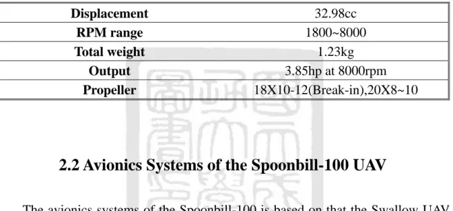
(23) Chapter 2 Spoonbill-100 UAV System In this chapter we will introduce the hardware and software of the Spoonbill100 UAV system. In addition, we also introduce the hardware-in-the-loop (HIL) simulation environment. The section on hardware describes the design concept and avionics system of the Spoonbill-100 UAV. The section on the software part introduces the HIL simulation environment and the ground control station (GCS).. 2.1 Design of the Spoonbill-100 UAV Section 2.1 presents an overview of the Spoonbill-100 UAV. The configuration of the Spoonbill-80 has been verified by almost one hundred flight tests, and it almost identical to that of the Spoonbill-100. However, we need an aircraft that can conduct a diving-airdrop, and it thus it must be lighter than the Spoonbill-80, while remaining strong. Therefore, the fuselage, main wing and tail wing were made of fiberglass, and the rods made of carbon. In addition, enlarged the fuselage of the vehicle so that the avionics system and airdrop box can be installed more easily. Table 2-1 shows the specifications of the Spoonbill-100. The Spoonbill-100 UAV weights 40% less than the Spoonbill-80 UAV, and thus we choose an O.S. GT-33 two-stroke gasoline engine to power it. This engine provides about 3.85 horsepower at 8000 rpm. Table 2-2 shows the specifications of the O.S. GT-33 gasoline engine.. 8.

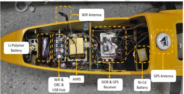
(24) Table 2-1 Specifications of Spoonbill-100 UAV NACA-63412 2.6 m 8 15 kg 6 kg O.S. GT-33. Main wing airfoil Main wing span Main wing aspect ration Maximum take-off weight Payload Engine. Table 2-2 Specifications of the O.S. GT-33 gasoline engine 32.98cc 1800~8000 1.23kg 3.85hp at 8000rpm 18X10-12(Break-in),20X8~10. Displacement RPM range Total weight Output Propeller. 2.2 Avionics Systems of the Spoonbill-100 UAV The avionics systems of the Spoonbill-100 is based on that the Swallow UAV system, with the redundant equipment having been removed. The avionics systems includes a computer, global positioning system (GPS), attitude and heading reference system (AHRS), serial (RS-232) to Wi-Fi adapter, air pressure sensor and sensor and servo input/output board (SIOB), and more detailed specification of these are presented below. Figure 2-1 shows the architecture of the avionics systems, and Figure 2-2 shows a photograph of it.. 9.

(25) Figure 2-1 The architecture of the avionics system. Figure 2-2 The avionics system of the Spoonbill-100. 10.

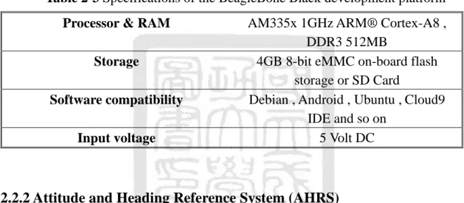
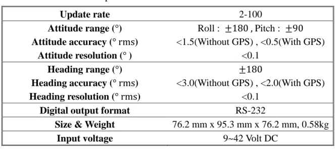
(26) 2.2.1 Computer The space inside a Spoonbill-100 is limited, and thus a small and light computer is needed to conduct the diving-airdrop experiment. We choose the BeagleBone Black development platform as the avionics computer, due to its small size and lightweight, and its Linux-based operating system. Table 2-3 shows the detailed specifications of the BeagleBone Black development platform.. Table 2-3 Specifications of the BeagleBone Black development platform AM335x 1GHz ARM® Cortex-A8 , DDR3 512MB 4GB 8-bit eMMC on-board flash storage or SD Card Debian , Android , Ubuntu , Cloud9 IDE and so on 5 Volt DC. Processor & RAM Storage Software compatibility Input voltage. 2.2.2 Attitude and Heading Reference System (AHRS) The attitude and heading are important to an aircraft during flight, and thus we need to obtain dynamic information about the Spoonbill-100. This is done using an attitude and heading reference system (AHRS) to help us to know the pitch, yaw, roll, and heading information, and the Crossbow AHRS440CA-200 is adopted for this. Table 2-4 shows the detailed specifications of the Crossbow AHRS440CA-200.. 11.

(27) Table 2-4 Specifications of the Crossbow AHRS440CA-200 2-100 Roll : ±180 , Pitch : ±90 <1.5(Without GPS) , <0.5(With GPS) <0.1 ±180 <3.0(Without GPS) , <2.0(With GPS) <0.1 RS-232 76.2 mm x 95.3 mm x 76.2 mm, 0.58kg 9~42 Volt DC. Update rate Attitude range (°) Attitude accuracy (° rms) Attitude resolution (° ) Heading range (°) Heading accuracy (° rms) Heading resolution (° rms) Digital output format Size & Weight Input voltage. 2.2.3 Global Positioning System (GPS) In addition to AHRS, the GPS receiver is an important sensor that provides the aircraft’s position to decide when to conduct the diving-airdrop, and it can also assist AHRS in correcting the attitude and heading. The GPS receiver is a NovAtel OEMV3 GNSS receiver, with the specifications shown in Table 2-5.. Table 2-5 Specifications of the NovAtel OEMV-3 GNSS receiver Length : 125 mm Width : 85 mm Height : 13 mm Weight : 75g GPS , GLONASS Single point L1,L1/L2 : 1.5m,1.2m SBAS : 0.6m DGPS : 0.4m RT-20, RT-2 L1TE, RT-2 : 0.2m, 2cm+1ppm, 1cm+1ppm Omni STAR VBS,XP,HP : 0.6m,0.15m,0.1m. Size & Weight. Constellation Performance accuracy (RMS). 12.

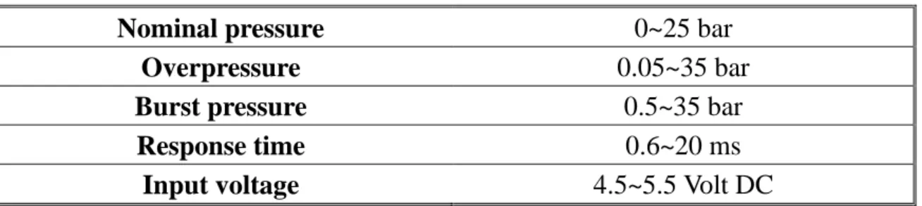
(28) 2.2.4 Sensor and Servo Input/Output Board (SIOB) RMRL designed a circuit board called a sensor and servo input/output board (SIOB) to integrate the information from sensors. The SIOB contains three Microchip 18F2580 peripheral interface controllers (PICs) and four relays. The first PIC decodes the pulse width modulation (PWM) signal sent by the RC receiver and receives the data from air pressure sensor. The second PIC receives the commands sent from the computer and converts these into inter-integrated circuit (I2 C) signals. The third PIC. controls the servos of the Spoonbill-100 using a I 2 C signal through four relays. These four relays are like four switches, and control the aileron, rudder, and elevator. and throttle signal independently. Figure 2-3 shows the SIOB, while Table 2-6 shows the specifications of the Senspecial SCPB series air pressure sensor.. Figure 2-3 Sensor and Servos Input/Output Board. 13.

(29) Table 2-6 Specifications of the Senspecial SCPB series air pressure sensor 0~25 bar 0.05~35 bar 0.5~35 bar 0.6~20 ms 4.5~5.5 Volt DC. Nominal pressure Overpressure Burst pressure Response time Input voltage. 2.2.5 RS-232 to Wi-Fi Adapter To send commands from the ground control station (GCS) and receive data from the Spoonbill-100, we set up an RS-232 to Wi-Fi adapter, which was installed inside the fuselage of the Spoonbill-100 and can send the data from SIOB, AHRS and GPS to another Wi-Fi adapter which set up near the ground control station, and vice versa.. 2.3 Ground Control Station The main function of the ground control station is providing a platform for upload command and monitoring real-time information about the Spoonbill-100 UAV. The ground control station includes two laptops, an RS-232 to Wi-Fi adapter and GCS program. The GCS program is programmed using Borland C++ Builder (BCB) and provides a graphical user interface (GUI), presenting a map, fuzzy controller parameters graphical display and details of the real-time conditions of the Spoonbill100 UAV. During flight tests one laptop is dedicated to monitoring the Spoonbill-100 and send our command to it. When ground test, the other laptop is dedicated to writing the GCS program and uploading it to the BeagleBone Black. The Figure 2-4 shows the GCS program. Figure 2-5 shows the ground control station.. 14.

(30) Figure 2-4 The GCS program. Figure 2-5 An overview of the ground control station (GCS). 15.

(31) 2.4 Hardware-in-the-Loop Simulation The HIL simulation is used to assess the controller, and it includes a desktop, a BeagleBone Black and the X-plane flight simulation software. After building the Spoonbill-100 model in the X-plane, it is used to simulate the flight test conditions to validate the performance of the controller. Figure 2-6 shows the architecture of the HIL simulation.. Figure 2-6 The architecture of the HIL simulation. 2.5 Summary This chapter described the avionics systems and specifications of the Spoonbill-100. It then explained how the model was built in X-plane and a program was written using C language and Borland C++ Builder to conduct the HIL simulation. However, a controller is needed to conduct the diving-airdrop, and this is explained in the next chapter. 16.

(32) Chapter 3 Spoonbill-100 UAV Diving-Airdrop System This chapter introduces the hardware and kinematics equations used in the Spoonbill-100 UAV diving-airdrop system. The diving-airdrop is the free fall type, and in the matrix laboratory (MATLAB) simulation we consider the influence of drag force. Therefore, in following sections, we will introduce the kinematics equation of diving-airdrop and present the simulation results obtained with MATLAB.. 3.1 Hardware of the Spoonbill-100 UAV Diving-Airdrop System In order to accomplish the diving-airdrop experiment, we need to build an airdrop-box and the payload. The airdrop-box has to be light, stable and, most importantly, it must be able to easily drop the payload. The payload needs to have a smooth surface and be made of a uniform material, with the center of mass located at the centroid. For these reasons we chose billiard balls as our payload. The diameter of each ball is 57mm, and the weight is about 0.172kg. Figure 3-1 shows the airdropbox, with the specifications shown in Table 3-1.. 17.

(33) Figure 3-1 The top view of the airdrop-box. Table 3-1 Specifications of the airdrop-box Length : 260 mm Width : 160 mm Height : 120 mm Weight : 0.325kg Diameter : 57mm Weight : 0.172kg. Size & Weight (Airdrop box). Size & Weight (Payload). 3.2 Coordinate Systems The GPS receiver board of the Spoonbill-100 UAV uses WGS84 to TWD97 [9] to navigate toward the target and calculate the distance from it. The coordinate system used for the equations of the diving-airdrop and Spoonbill-100 during the flight tests is a body coordinate system, which follows the right-hand rule with mutually orthogonal axes.. 18.

(34) 3.2.1 World Geodetic System WGS84 is the reference coordinate system used by the GPS. In our experiment, the GPS receive board receives the signal sent by satellites and records the position of the Spoonbill-100 in WGS84 format (i.e., Longitude, Latitude and Altitude). The 𝜆𝜆 position vector in the geodetic coordinate system is denoted by �𝜑𝜑�, where 𝜆𝜆 is ℎ. latitude, 𝜑𝜑 is longitude and h is altitude. Figure 3-2 shows the WGS84 reference frame.. Figure 3-2 The WGS 84 reference frame. 19.

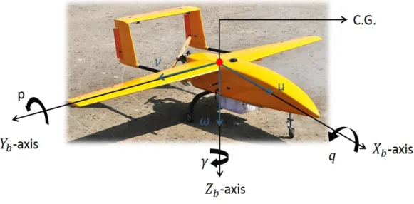
(35) 3.2.2 Body Coordinate System The body coordinate system is defined based on the aircraft, and therefore the origin of the system is the center of gravity (CG) of the aircraft. The 𝑋𝑋𝑏𝑏 -axis points parallel toward to the nose, the 𝑌𝑌𝑏𝑏 -axis points parallel toward to the right wing and. the 𝑍𝑍𝑏𝑏 -axis points parallel toward the bottom of the aircraft. The roll, pitch and yaw are positive with the 𝑋𝑋𝑏𝑏 , 𝑌𝑌𝑏𝑏 and 𝑍𝑍𝑏𝑏 axies in right-hand rule. Figure 3-3 shows the. notations for the velocity and angular velocity in body coordinate system.. Figure 3-3 The notations for the velocity and angular velocity in the body coordinate system. 3.3 Equation of Motion of Diving-Airdrop In this thesis, the payloads are uniform spheres with a smooth surface rigid body, therefore we assume the force is acting at the center of gravity. In most airdrop case, the whole motion of the projectile is in one plane. Thus, the dimensional space of projectile motion is two-dimensional (2D). In this thesis, the vertical displacement of the projectile motion is much smaller than the radius of the earth and for many 20.

(36) problems such as aircraft simulation the gravity acceleration is a constant g = 9.80665 �𝑚𝑚�𝑠𝑠 2 � [10]. We use the rectangular coordinate to represent the position (3.1),. velocity (3.2) and acceleration (3.3). The X-axis direction is the direction of the. diving-airdrop payload’s throw distance (TD), and the Z-axis direction is the falling direction of the payload. The Figure 3-4 shows the free body diagram of the divingairdrop.. Figure 3-4 The free body diagram of the diving-airdrop. 𝑟𝑟 = 𝑥𝑥𝑥𝑥 + 𝑦𝑦𝑦𝑦 + 𝑧𝑧𝑧𝑧. (3.1). 𝑟𝑟̈ = 𝑥𝑥̈ 𝑖𝑖 + 𝑦𝑦̈ 𝑗𝑗 + 𝑧𝑧̈ 𝑘𝑘. (3.3). 𝑟𝑟̇ = 𝑥𝑥̇ 𝑖𝑖 + 𝑦𝑦̇ 𝑗𝑗 + 𝑧𝑧̇ 𝑘𝑘. (3.2). From Figure 3-4, we know that the origin of the coordinate is at the center of gravity. The gravity force “mg” and the drag force “𝐹𝐹𝑑𝑑 ” are acting at the center of gravity, and “θ” is the initial pitch angle when the UAV drops the payload.. 21.

(37) As noted above, the payload is affected by gravity and drag force. From Newton’s second law, we have (3.4) and (3.5) and sum the external forces up in Xaxis direction (3.6) and Z-axis direction (3.7).. Σ𝐹𝐹𝑥𝑥 = m𝑎𝑎𝑥𝑥 = 𝑚𝑚𝑥𝑥̈. (3.4). Σ𝐹𝐹𝑧𝑧 = m𝑎𝑎𝑧𝑧 = 𝑚𝑚𝑧𝑧̈. (3.5). 𝑚𝑚𝑧𝑧̈ + 𝑚𝑚𝑚𝑚 − 𝐹𝐹𝑑𝑑 ∙ 𝑠𝑠𝑠𝑠𝑠𝑠𝑠𝑠 = 0. (3.7). 𝑚𝑚𝑥𝑥̈ − 𝐹𝐹𝑑𝑑 ∙ 𝑐𝑐𝑐𝑐𝑐𝑐𝑐𝑐 = 0. (3.6). Therefore, the equations of motion of the diving-airdrop could be represented in (3.8) and (3.9), as follows: 𝑋𝑋 − 𝑎𝑎𝑎𝑎𝑎𝑎𝑎𝑎 𝑑𝑑𝑑𝑑𝑑𝑑𝑑𝑑𝑑𝑑𝑑𝑑𝑑𝑑𝑑𝑑𝑑𝑑 ∶ 𝑚𝑚𝑥𝑥̈ − 𝐹𝐹𝐹𝐹 ∙ 𝑐𝑐𝑐𝑐𝑐𝑐𝑐𝑐 = 0. 𝑍𝑍 − 𝑎𝑎𝑎𝑎𝑎𝑎𝑎𝑎 𝑑𝑑𝑑𝑑𝑑𝑑𝑑𝑑𝑑𝑑𝑑𝑑𝑑𝑑𝑑𝑑𝑑𝑑 ∶ 𝑚𝑚𝑧𝑧̈ + 𝑚𝑚 �𝑔𝑔 −. 𝐹𝐹𝐹𝐹∙𝑠𝑠𝑠𝑠𝑠𝑠𝑠𝑠 𝑚𝑚. (3.8). � =0. (3.9). From (3.8) and (3.9), the acceleration of the X-axis is 𝑎𝑎𝑥𝑥 = 𝑥𝑥̈ =. of Z-axis is 𝑎𝑎𝑧𝑧 = 𝑧𝑧̈ = -g +. 𝐹𝐹𝐹𝐹∙𝑠𝑠𝑠𝑠𝑠𝑠𝑠𝑠 𝑚𝑚. 𝐹𝐹𝐹𝐹∙𝑐𝑐𝑐𝑐𝑐𝑐𝑐𝑐 𝑚𝑚. and that. . Using fluid mechanics, the drag force is obtained. based on the drag coefficient (𝐶𝐶𝑑𝑑 ), reference area (A), density of the fluid (ρ) and. velocity of object relative to the fluid (ν), as seen in (3.10).. 1. 𝐹𝐹𝐹𝐹 = ∙ 𝜌𝜌 ∙ 𝐶𝐶𝑑𝑑 ∙ A ∙ 𝜈𝜈 2 2. (3.10). In the general experimental condition, the temperature is about 20°C~35°C (293K~308K) and the air density at sea level is 1.174 �. 𝑘𝑘𝑘𝑘. 𝑚𝑚3. � [11]. The Reynolds. number (R e ) can be calculated according to the Sutherland's law [12], and it is 3.65×. 103 × 𝜈𝜈.. 22.

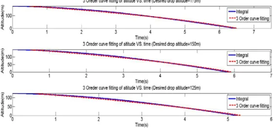
(38) In the experiment, the range of velocity is about 22~35 (𝑚𝑚⁄𝑠𝑠) during flight.. Therefore, the range of the Reynolds number (R e ) is about 7.1731 × 104 < 𝑅𝑅𝑒𝑒 < 1.2775 × 105 and the drag coefficient of a smooth sphere is near a constant 0.47,. based on research carried out by of NASA [13].. Figure 3-5 The drag coefficient of a sphere [13]. In addition, we can derive the falling time and throw distance during a divingairdrop with the kinematics equations (3.11), (3.12) and (3.13). ν = 𝜈𝜈0 + 𝑎𝑎𝑎𝑎. (3.11). 𝜈𝜈 2 = 𝜈𝜈0 2 + 2𝑎𝑎Δ𝑥𝑥. Δ𝑥𝑥 = 𝜈𝜈0 𝑡𝑡 +. 1 2. 𝑎𝑎𝑡𝑡 2. (3.12) (3.13). During the diving-airdrop, the notation for altitude is “h” and the initial velocity in the Z-axis direction is “νsin(θ)”. We next solve the kinematics equations to get the. falling time and throw distance (TD):. 23.

(39) 𝑡𝑡𝑓𝑓𝑓𝑓𝑓𝑓𝑓𝑓 =. 1. −𝜈𝜈sin(𝜃𝜃)±�(𝜈𝜈sin(𝜃𝜃))2 +4×2×𝑎𝑎𝑧𝑧 ×ℎ. TD = 𝜈𝜈 cos(𝜃𝜃) × 𝑡𝑡𝑓𝑓𝑓𝑓𝑓𝑓𝑓𝑓 + 𝑣𝑣. 𝜃𝜃𝑣𝑣 = arctan � 𝑧𝑧 � 𝑣𝑣𝑥𝑥. 𝑎𝑎𝑧𝑧 1 2. (3.14). × 𝑎𝑎𝑥𝑥 × 𝑡𝑡𝑓𝑓𝑓𝑓𝑓𝑓𝑓𝑓 2 (3.15). (3.16). From (3.14), (3.15) and (3.16) we can see that the pitch angle, velocity, altitude and acceleration change during diving-airdrop and affect 𝑡𝑡𝑓𝑓𝑓𝑓𝑓𝑓𝑓𝑓 and TD. We use. MATLAB to simulate the diving-airdrop for 20 seconds and calculate the drag force, velocity of X-axis, velocity of Z-axis, etc. Then, we have three order curve fitting equations of altitude VS. 𝑡𝑡𝑓𝑓𝑓𝑓𝑓𝑓𝑓𝑓 and 𝑡𝑡𝑓𝑓𝑓𝑓𝑓𝑓𝑓𝑓 VS. TD that we can use in the diving-. airdrop code for outdoor experiment. The following tables and figures present curve fitting equations.. Table 3-2 The three order curve fitting equations (Desired drop pitch angle = 𝟎𝟎° ). Altitude VS. Time Time VS. Throw distance. Altitude VS. Time Time VS. Throw distance. Altitude VS. Time Time VS. Throw distance. Altitude = 175m t = -3.501× 10−7 ℎ3 -2.377× 10−5 ℎ2 0.0208h+6.9439 3 x = 0.0283𝑡𝑡 − 1.5511𝑡𝑡 2 + 28.2499𝑡𝑡 − 0.1905 Altitude = 150m t = -3.501× 10−7 ℎ3 -5.0031× 10−5 ℎ2 0.0226h+6.4047 3 x = 0.0283𝑡𝑡 − 1.5511𝑡𝑡 2 + 28.2499𝑡𝑡 − 0.1905 Altitude = 125m t = -3.501× 10−7 ℎ3 -7.6288× 10−5 ℎ2 0.0258h+5.8030 x = 0.0283𝑡𝑡 3 − 1.5511𝑡𝑡 2 + 28.2499𝑡𝑡 − 0.1905 24.

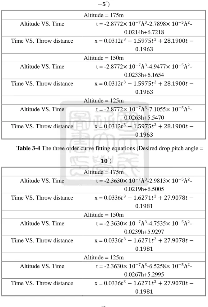
(40) Table 3-3 The three order curve fitting equations (Desired drop pitch angle = −𝟓𝟓° ). Altitude VS. Time Time VS. Throw distance. Altitude VS. Time Time VS. Throw distance. Altitude VS. Time Time VS. Throw distance. Altitude = 175m t = -2.8772× 10−7 ℎ3 -2.7898× 10−5 ℎ2 0.0214h+6.7218 x = 0.0312𝑡𝑡 3 − 1.5975𝑡𝑡 2 + 28.1900𝑡𝑡 − 0.1963 Altitude = 150m t = -2.8772× 10−7 ℎ3 -4.9477× 10−5 ℎ2 0.0233h+6.1654 x = 0.0312𝑡𝑡 3 − 1.5975𝑡𝑡 2 + 28.1900𝑡𝑡 − 0.1963 Altitude = 125m t = -2.8772× 10−7 ℎ3 -7.1055× 10−5 ℎ2 0.0263h+5.5470 x = 0.0312𝑡𝑡 3 − 1.5975𝑡𝑡 2 + 28.1900𝑡𝑡 − 0.1963. Table 3-4 The three order curve fitting equations (Desired drop pitch angle = −𝟏𝟏𝟏𝟏° ). Altitude VS. Time Time VS. Throw distance. Altitude VS. Time Time VS. Throw distance. Altitude VS. Time Time VS. Throw distance. Altitude = 175m t = -2.3630× 10−7 ℎ3 -2.9813× 10−5 ℎ2 0.0219h+6.5005 x = 0.0336𝑡𝑡 3 − 1.6271𝑡𝑡 2 + 27.9078𝑡𝑡 − 0.1981 Altitude = 150m t = -2.3630× 10−7 ℎ3 -4.7535× 10−5 ℎ2 0.0239h+5.9297 x = 0.0336𝑡𝑡 3 − 1.6271𝑡𝑡 2 + 27.9078𝑡𝑡 − 0.1981 Altitude = 125m t = -2.3630× 10−7 ℎ3 -6.5258× 10−5 ℎ2 0.0267h+5.2995 x = 0.0336𝑡𝑡 3 − 1.6271𝑡𝑡 2 + 27.9078𝑡𝑡 − 0.1981 25.

(41) Figure 3-6 The altitude VS. time three order curve fitting equations (Desired drop pitch angle = 0° ). Figure 3-7 The altitude VS. time three order curve fitting equations (Desired drop pitch angle = 0° ) 26.

(42) Figure 3-8 The time VS. throw distance three order curve fitting equations (Desired drop pitch angle = −5° ). Figure 3-9 The time VS. throw distance three order curve fitting equations (Desired drop pitch angle = −5° ) 27.

(43) Figure 3-10 The altitude VS. time three order curve fitting equations (Desired drop pitch angle = −10° ). Figure 3-11 The time VS. throw distance three order curve fitting equations (Desired drop pitch angle = −10° ). 28.

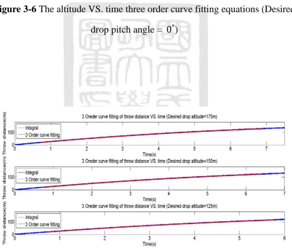
(44) Therefore, we simulate the diving-airdrop using an integral method in MATLAB to calculate 𝑡𝑡𝑓𝑓𝑓𝑓𝑓𝑓𝑓𝑓 and TD. In addition, we use MATLAB to simulate the 𝜃𝜃𝑣𝑣 and. velocity during a diving-airdrop for 20 seconds when affected by the drag force, without the drag force and the change of drag force during a diving-airdrop. The results show that when the altitude decreases by 25m that TD falls by 7m~8m and the falling time declines 0.6s. When pitch angle decreases by −5° the TD falls by. 4m~5m and the falling time declines by 0.3s. From these results we can determine the appropriate timing to conduct a diving-airdrop. Table 3-5 The 𝒕𝒕𝒇𝒇𝒇𝒇𝒇𝒇𝒇𝒇 and TD at altitude =175m Pitch angle 0° −5° −10° Pitch angle 0° −5° −10° Pitch angle 0° −5° −10°. Falling time(𝑪𝑪𝒅𝒅 ) 6.9120s 6.6740s 6.4440s. Altitude=175m Throw Pitch Falling distance(𝑪𝑪𝒅𝒅 ) angle time(No 𝑪𝑪𝒅𝒅 ) 130.2887m 5.9750s 0° ° 126.0487m 5.7310s −5 121.0679m 5.4990s −10°. Throw distance(No 𝑪𝑪𝒅𝒅 ) 167.3m 159.8574m 151.6328m. Altitude=150m Throw Pitch Falling distance(𝑪𝑪𝒅𝒅 ) angle time(No 𝑪𝑪𝒅𝒅 ) 123.3516m 5.5310s 0° ° 118.9858m 5.2880s −5 113.9542m 5.0580s −10°. Throw distance(No 𝑪𝑪𝒅𝒅 ) 154.8680m 147.5006m 139.4724m. Altitude=125m Throw Pitch Falling distance(𝑪𝑪𝒅𝒅 ) angle time(No 𝑪𝑪𝒅𝒅 ) 115.2642m 5.0500s 0° 110.7635m 4.8070s −5° ° 105.6720m 4.5780s −10. Throw distance(No 𝑪𝑪𝒅𝒅 ) 141.4000m 134.0838m 126.2366m. Table 3-6 The 𝒕𝒕𝒇𝒇𝒇𝒇𝒇𝒇𝒇𝒇 and TD at altitude =150m Falling time(𝑪𝑪𝒅𝒅 ) 6.3020s 6.0630s 5.8340s. Table 3-7 The 𝒕𝒕𝒇𝒇𝒇𝒇𝒇𝒇𝒇𝒇 and TD at altitude =125m Falling time(𝑪𝑪𝒅𝒅 ) 5.6630s 5.4240s 5.1960s. 29.

(45) Figure 3-12 The TD VS. pitch angle at altitude 175m. Figure 3-13 The TD VS. pitch angle at altitude 150m. 30.

(46) Figure 3-14 The TD VS. pitch angle at altitude 125m. Figure 3-15 MATLAB simulates drag force during diving-airdrop for 20 seconds. Here, we simulate the 𝜃𝜃𝑣𝑣 , the velocity of X-axis, the velocity of Z-axis and the. velocity during diving-airdrop with the effect of drag force and without drag force for 20 seconds by MATLAB. We can see how the drag force affects the payload in 31.

(47) Figures 3-16~19. With the effect of drag force, the final 𝜃𝜃𝑣𝑣 of the payload is almost. 90° and the final velocity is about 48𝑚𝑚⁄𝑠𝑠. Without the effect of drag force, the final. 𝜃𝜃𝑣𝑣 of the payload is almost 80° and the final velocity is about 200𝑚𝑚⁄𝑠𝑠.. Figure 3-16 MATLAB simulates 𝜃𝜃𝑣𝑣 during diving-airdrop for 20 seconds. Figure 3-17 MATLAB simulates velocity of X-axis during diving-airdrop for 20 seconds 32.

(48) Figure 3-18 MATLAB simulates velocity of Z-axis during diving-airdrop for 20 seconds. Figure 3-19 MATLAB simulates velocity of X-axis during diving-airdrop for 20 seconds. 33.

(49) 3.4 Method and Controllers of the Diving-airdrop System The section presents the method used to conduct a diving-airdrop. Figure 3-20 shows the architecture of the diving-airdrop system and the system as a whole to obtain the dynamic data of the Spoonbill-100, including the GPS position, airspeed and altitude. The avionics computer then calculates the TD and UAV to target distance (UTD). When UTD< TD, the avionics computer sends a command to open the gate of the airdrop-box and drop the payload. As it is difficult to maintain the UAV at exactly the desired altitude before an autonomous diving-airdrop takes place, we thus set the altitude restriction to decide the timing of diving-airdrop. Airdrop box open: UTD < TD and Desired altitude -25 < Desired altitude < Desired altitude +15 Airdrop box close: UTD > TD or Desired altitude > Desired altitude +15 or Desired altitude < Desired altitude -25. 34.

(50) Figure 3-20 The architecture of the diving-airdrop system. Figure 3-21 Side view of diving-airdrop. In this thesis, the controllers are two input and one output fuzzy controllers. These are the aileron controller, elevator controller and throttle controller. In the aileron controller, the two inputs include the error of the roll angle and rate of roll angle change, and the one output is the aileron PWM signal. In the altitude controller, the two inputs include the error of the pitch angle and the rate of pitch angle change, and the one output is the elevator PWM signal. In the throttle controller, the two inputs include the error of airspeed and rate of altitude change, and the one output is throttle PWM signal, but we only use the throttle controller in HIL simulation. Figures 3-22~24 show the block diagrams of the aileron, elevator and throttle fuzzy controllers.. 35.

(51) Figure 3-22 Block diagram of the elevator fuzzy controller. Figure 3-23 Block diagram of the aileron fuzzy controller. Figure 3-24 Block diagram of the throttle fuzzy controller. 36.

(52) Chapter 4 HIL Simulation Results and Experiment Results for Diving-Airdrops In this chapter we will present the results of the HIL simulation and the experiment. In the HIL simulation, we set the range of altitude from 125m~175m, the range of pitch angle from 0° ~ − 10° and the velocity is maintained at 28(𝑚𝑚⁄𝑠𝑠). In the diving-airdrop experiment, we keep the range of altitude from 125~175m, and the. range of pitch angle from −5° ~ − 10° and the velocity is maintained 28m/s. There are nine HIL simulation data and six experimental data.. 4.1 HIL Simulation Results We conduct an HIL simulation to make sure the fuzzy controller of the divingairdrop can be used, and thus reduce the risk during flight tests. Since the X-plane does not have Cigu, Tainan, which is the location of the flight test, we replace this with Tainan Airport. Figure 4-1 shows a top view of the airport, and we can see the flying direction during the HIL simulation and the position of the target.. 37.

(53) Figure 4-1 Top view of Tainan airport. In the HIL simulation, we use the TD and the UAV’s current position to predict the impact point. The rate of data collection in HIL is 20Hz and the data log shows that the UTD changes by about 6~8 meters in each data interval. We thus set a reasonable radius of drop zone in HIL at 5 meters. To make it easier to know the error distance between the impact point and target, we have to transform the WGS 84 into TWD 97 format. Figure 4-2 shows the method used to predict the impact point, while the equations 4.1~.2 show the UTD and error distance.. UTD : �(𝑥𝑥1 − 𝑥𝑥3 )2 + (𝑦𝑦1 − 𝑦𝑦3 )2. Error distance : �(𝑥𝑥2 − 𝑥𝑥3 )2 + (𝑦𝑦2 − 𝑦𝑦3 )2 38. (4.1) (4.2).

(54) Tables 4-1~4-3 show the results of the HIL simulation, such as the TD, payload dropping time and so on. Using this that we can design the logic with regard to timing the diving-airdrop.. Figure 4-2 The method for predicting the impact point. Table 4-1 The data for the HIL simulation when the desired drop altitude = 175m No. Altitude Pitch angle Airspeed. 1. 175.253 m 0.3109° 28.19. 2. 176.513 m −4.4676°. 𝑚𝑚. 29.87. 𝑠𝑠. 𝑚𝑚 𝑠𝑠. 3. 177.866 m −10.5947° 30.48. 𝑚𝑚 𝑠𝑠. Throw distance 130.620 m 127.085 m 122.815 m Error distance 1.097 m 1.811 m 2.803 m Falling time 6.940s 6.767s 6.607s Target (120.207951,22 (120.207951,22 (120.207951,22 .938008) .938008) .938008) Impact point (120.207997,22 (120.207955,22 (120.207957,22 .936849) .938107) .938118) 39.

(55) Table 4-2 The data for the HIL simulation when the desired drop altitude = 150m No. Altitude Pitch angle Airspeed. 4. 150.545 m 0.2168° 28.13. 5. 151.775 m −5.2878°. 𝑚𝑚. 29.53. 𝑠𝑠. 𝑚𝑚 𝑠𝑠. 6. 153.027 m −10.1438° 30.48. 𝑚𝑚 𝑠𝑠. Throw distance 124.690 m 120.869 m 116.444 m Error distance 1.415 m 1.093 m 1.930 m Falling time 6.416s 6.222s 6.043s Target (120.207951,22 (120.207951,22 (120.207951,22 .938008) .938008) .938008) Impact point (120.207958,22 (120.207959,22 (120.207959,22 .938028) .938100) .938109). Table 4-3 The data for the HIL simulation when the desired drop altitude = 125m No. Altitude Pitch angle Airspeed. 7. 125.256 m −0.0772° 28.08. 8. 126.266 m −4.5155°. 𝑚𝑚. 29.86. 𝑠𝑠. 𝑚𝑚 𝑠𝑠. 9. 127.627 m −9.5312° 30.55. 𝑚𝑚 𝑠𝑠. Throw distance 117.159 m 112.989 m 108.488 m Error distance 2.867 m 0.725 m 0.776 m Falling time 5.812s 5.595s 5.411s Target (120.207951,22 (120.207951,22 (120.207951,22 .938008) .938008) .938008) Impact point (120.207985,22 (120.207963,22 (120.207970,22 .937938) .938100) .938086). 40.

(56) To examine the performance of the aileron controller, elevator controller and throttle controller we analyze the error between the desired and measured values of pitch angle, roll angle, altitude and airspeed. We compare the error with mean error, root mean square (RMS) and standard deviation. Tables 4-4~4-6 show the error of the HIL simulation, and it can be seen that the mean error of pitch angle, roll angle, altitude and airspeed are almost all in the range of one standard deviation. The RMS of the pitch angle, roll angle, altitude and airspeed are located in the interval between one to two standard deviations. Table 4-4 The error the HIL simulation when the desired drop altitude = 175m Error Pitch angle Roll angle Altitude Airspeed. Error Pitch angle Roll angle Altitude Airspeed. Error Pitch angle Roll angle Altitude Airspeed. Desired drop pitch angle = 0° Mean error RMS 0.0714° 0.1784° 0.2911° 1.8633° 0.0572m 0.1381m 0.0246. 𝑚𝑚. 0.0627. 𝑠𝑠. 𝑚𝑚. Standard deviation 0.1508° 1.8223° 0.1150m 0.0534. 𝑠𝑠. Desired drop pitch angle = −5° Mean error RMS. 𝑚𝑚 𝑠𝑠. 0.8825° 0.2059° 0.1565m. 1.3699° 0.3370° 0.2495m. Standard deviation 0.8722° 0.2309° 0.1656m. 0.0663. 0.1046. 0.0684. 𝑚𝑚 𝑠𝑠. 𝑚𝑚 𝑠𝑠. Desired drop pitch angle = −10° Mean error RMS. 𝑚𝑚 𝑠𝑠. 1.1103° 0.2275° 0.2221m. 1.7323° 0.3733° 0.3829m. Standard deviation 1.1185° 0.2566° 0.2767m. 0.0894. 0.1481. 0.1030. 𝑚𝑚 𝑠𝑠. 41. 𝑚𝑚 𝑠𝑠. 𝑚𝑚 𝑠𝑠.

(57) Table 4-5 The error of the HIL simulation when the desired drop altitude = 150m Error Pitch angle Roll angle Altitude Airspeed. Error Pitch angle Roll angle Altitude Airspeed. Error Pitch angle Roll angle Altitude Airspeed. Desired drop pitch angle = 0° Mean error RMS 0.0038° 0.0284° 0.0063° 0.0504° 0.0167m 0.1194m 0.0056. 𝑚𝑚. 0.0394. 𝑠𝑠. 𝑚𝑚. Standard deviation 0.0279° 0.0496° 0.1171m 0.0386. 𝑠𝑠. Desired drop pitch angle = −5° Mean error RMS. 𝑚𝑚 𝑠𝑠. 0.8138° 0.1698° 0.1382m. 1.3830° 0.3082° 0.2486m. Standard deviation 0.9463° 0.2252° 0.1802m. 0.0588. 0.1062. 0.0773. 𝑚𝑚 𝑠𝑠. 𝑚𝑚 𝑠𝑠. Desired drop pitch angle = −10° Mean error RMS. 𝑚𝑚 𝑠𝑠. 0.7868° 0.1814° 0.1488m. 1.3762° 0.3161° 0.3026m. Standard deviation 0.9829° 0.2249° 0.2416m. 0.0624. 0.1167. 0.0882. 𝑚𝑚 𝑠𝑠. 42. 𝑚𝑚 𝑠𝑠. 𝑚𝑚 𝑠𝑠.

(58) Table 4-6 The error of the HIL simulation when the desired drop altitude = 125m Error Pitch angle Roll angle Altitude Airspeed. Error Pitch angle Roll angle Altitude Airspeed. Error Pitch angle Roll angle Altitude Airspeed. Desired drop pitch angle = 0° Mean error RMS 0.0224° 0.1115° 0.0168° 0.0902° 0.0390m 0.2035m 0.0129. 𝑚𝑚. 0.0635. 𝑠𝑠. 𝑚𝑚. Standard deviation 0.1070° 0.0871° 0.1961m 0.0609. 𝑠𝑠. Desired drop pitch angle = −5° Mean error RMS. 𝑚𝑚 𝑠𝑠. 0.7080° 0.1515° 0.1256m. 1.2808° 0.2830° 0.2361m. Standard deviation 0.9254° 0.2103° 0.1763m. 0.0536. 0.0989. 0.0727. 𝑚𝑚 𝑠𝑠. 𝑚𝑚 𝑠𝑠. Desired drop pitch angle = −10° Mean error RMS. 𝑚𝑚 𝑠𝑠. 0.6937° 0.1667° 0.1263m. 1.3275° 0.2998° 0.2837m. Standard deviation 1.0099° 0.2167° 0.2363m. 0.0625. 0.1230. 0.0953. 𝑚𝑚 𝑠𝑠. 43. 𝑚𝑚 𝑠𝑠. 𝑚𝑚 𝑠𝑠.

(59) 4.2 Experimental Result To validate the performance of the diving-airdrop system of the Spoonbill100, we conduct six diving-airdrop experiments and drop the payload at altitudes of 175m, 150m and 125m with pitch angles of −5° and −10° . Figure 4-3 shows the experimental site on 2014/10/31 at Cigu, Tainan. As the UAV does not have the ability to automatically take-off, we hired an experienced radio controlled airplane user as our pilot to control the UAV at an appropriate altitude and the switch it into automatic diving-airdrop mode. Tables 4-7~8 and Figures 4-4~14 show the flight data.. Figure 4-3 The experimental site on 2014/10/31 at Cigu, Tainan, from Google Map. 44.

(60) Table 4-7 The flight data on 2014/10/31, No.1 ~ 3. No. Altitude Pitch angle Airspeed. 1. 182.181 m −1.7908° 28.97. 2. 160.904 m 0.4065°. 𝑚𝑚. 32.05. 𝑠𝑠. 𝑚𝑚 𝑠𝑠. 3. 132.747 m −1.9116° 31.08. 𝑚𝑚 𝑠𝑠. Throw distance 145.664 m 152.428 m 133.887 m Error distance 28.676 m 29.654 m 28.800 m (Computer) Error distance 36.35m 32.7m 25.8m (Measure) Falling time 6.004s 5.705s 5.099s Impact point (120.094164,23 (120.094456,23 (120.094628,23 (Computer) .156427) .156578) .156484) Impact point (120.094397,23 (120.094498,23 (120.094482,23 (Measure) .156015) .156041) .156086). Table 4-8 The flight data on 2014/10/31, No.4 ~ 6. No. Altitude Pitch angle Airspeed. 4. 187.975 m −1.5820° 31.83. 5. 161.139 m −0.3735°. 𝑚𝑚. 31.33. 𝑠𝑠. 𝑚𝑚 𝑠𝑠. 6. 135.973 m 4.5154° 33.44. 𝑚𝑚 𝑠𝑠. Throw distance 160.864 m 149.476 m 124.934 m Error distance 28.676 m 10.846 m 29.367 m (Computer) Error distance 31.45m 18.25m 29.8m (Measure) Falling time 6.103s 5.712s 5.037s Impact point (120.094529,23 (120.094476,23 (120.094420,23 (Computer) .156524) .156232) .156577) Impact point (120.094605,23 (120.094548,23 (120.094477,23 (Measure) .156068) .156175) .156065). 45.

(61) Figure 4-4 The pitch, roll and heading on 2014-10-31 flight test, No.1. Figure 4-5 The pitch, roll and heading on 2014-10-31 flight test, No.2. 46.

(62) Figure 4-6 The pitch, roll and heading on 2014-10-31 flight test, No.3. Figure 4-7 The altitude on 2014-10-31 flight test, No.1 ~ 3. 47.

(63) Figure 4-8 The flight trace on 2014-10-31 flight test, No.1 ~ 3. Figure 4-9 The altitude on 2014-10-31 flight test, No.4. 48.

(64) Figure 4-10 The altitude on 2014-10-31 flight test, No.5. Figure 4-11 The altitude on 2014-10-31 flight test, No.6. 49.

(65) Figure 4-12 The altitude on 2014-10-31 flight test, No.4 ~ 6. Figure 4-13 The flight trace on 2014-10-31 flight test, No.4 ~ 6. 50.

(66) Figure 4-14 The impact points on 2014-10-31 flight test. 4.3 Discussion In this section, we discuss the effect of altitude, pitch angle, velocity and wind, based on the results obtained with MATLAB, and the cause of any errors with regard to the impact point and target. 1. Effects of changes in altitude We set the velocity at 28 (𝑚𝑚⁄𝑠𝑠)and pitch angle at 0° . In addition, we set the. altitude at 175m, 150m and 125m as the standard and plus or minus 3 m to see the effects of the changes in this. Table 4-9 shows that when there is a 1m change in altitude, the range of TD changes by about 0.25~0.35m.. 51.

(67) Table 4-9 The effects of changes in altitude Drop velocity = 28 𝑚𝑚⁄𝑠𝑠 & Drop pitch angle = 0° Altitude(m) TD(m) Error distance(m) 178 131.0490 0.7603 177 130.8038 0.5151 176 130.5468 0.2581 175 130.2887 0 174 130.0295 -0.2592 173 129.7692 -0.5195 172 129.5079 -0.7808 Altitude(m) TD(m) Error distance(m) 153 124.2328 0.8812 152 123.9364 0.5848 151 123.6387 0.2871 150 123.3516 0 149 123.0514 -0.3002 148 122.7499 -0.6017 147 122.4471 -0.9045 Altitude(m) TD(m) Error distance(m) 128 116.2984 1.0342 127 115.9551 0.6909 126 115.6104 0.3462 125 115.2642 0 124 114.9164 -0.3478 123 114.5538 -0.7104 122 114.2030 -1.0612. 52.

(68) 2. Effects of changes in pitch angle We set the velocity at 28 𝑚𝑚⁄𝑠𝑠 and altitude at175m. In addition, we set the. altitude at 0° , −5° and −10° as the standard and plus or minus 2° to see the. effects of changes in pitch angle. Table 4-10 shows that when there is a change 1° of pitch angle the range of TD changes about by 0.75~1.1m.. Table 4-10 The effects of changes in pitch angle Drop velocity = 28 𝑚𝑚⁄𝑠𝑠 & Drop altitude = 175m Pitch angle (deg) TD(m) Error distance(m) 131.7551 1.4664 2° ° 131.0349 0.7462 1 130.2887 0 0° 129.5063 -0.7824 −1° ° 128.6883 -1.6004 −2 Pitch angle (deg) TD(m) Error distance(m) ° 127.8352 1.7868 −3 ° 126.9587 0.9103 −4 126.0484 0 −5° ° 125.1050 -0.9434 −6 124.1400 -1.9084 −7° Pitch angle (deg) TD(m) Error distance(m) ° 123.1432 2.0759 −8 122.1151 1.0478 −9° ° 121.0673 0 −10 ° 119.9896 -1.0777 −11 118.8824 -2.1849 −12°. 53.

(69) 3. Effects of changes in velocity We set the pitch angle at 0° and altitude at 175m. In addition, we set the velocity. of 28 𝑚𝑚⁄𝑠𝑠 as the standard and plus 7 𝑚𝑚⁄𝑠𝑠 or minus 6 𝑚𝑚⁄𝑠𝑠 to see the effects of changes in velocity. Table 4-11 shows that when there is a change 1𝑚𝑚⁄𝑠𝑠 in velocity, the range of TD changes by about 3.5~4.2m.. Table 4-11 The effects of changes in velocity Drop altitude = 175m & Drop pitch angle = 0° Velocity (𝑚𝑚⁄𝑠𝑠) TD (m) Error distance (m) 22 105.8434 -24.4453 23 110.0358 -20.2529 24 114.1858 -16.1029 25 118.2852 -12.0035 26 122.3247 -7.964 27 126.3358 -3.9529 28 130.2887 0 29 134.1945 3.9058 138.0542 7.7655 30 141.8570 11.5683 31 32 145.6266 15.3379 33 149.3527 19.064 34 153.0361 22.7474 35 156.6776 26.3889. 54.

(70) 4. Effects of wind We set the pitch angle at 0° , velocity at 28𝑚𝑚⁄𝑠𝑠, and altitude at 125m, 150m and. 175m. In addition, we set the no wind condition as standard and plus 10 knots (5.144𝑚𝑚⁄𝑠𝑠) wind or minus 10 knots (5.144𝑚𝑚⁄𝑠𝑠) to see the effects of change in wind speed. Table 4-12 shows that under the 10 knots (5.144𝑚𝑚⁄𝑠𝑠) wind condition the range of TD changes by about 17.6~20.8m.. Table 4-12 The effects of wind Drop pitch angle = 0° , drop velocity = 28𝑚𝑚⁄𝑠𝑠 & No wind Altitude (m) TD (m) Error distance (m) 175 130.2887 0 150 122.4471 0 125 114.2030 0 ° 𝑚𝑚 Drop pitch angle = 0 , drop velocity = 28 ⁄𝑠𝑠 & wind direction (0° ) 175 109.4380 -20.8507 150 103.4883 -18.9588 125 96.5580 -17.645 ° Drop pitch angle = 0 , drop velocity = 28𝑚𝑚⁄𝑠𝑠 & wind direction (180° ) 175 149.8925 19.6038 150 142.0797 19.6326 125 132.9632 18.7602. 55.

(71) Based on the discussion above and outdoor experiment, we can obtain the following results. 1. The average error distance in the HIL simulation is 1.919m. The reason is the rate of data collection is 20Hz and the average velocity is 29.443𝑚𝑚⁄𝑠𝑠.. Therefore, the aircraft moves about 1.5m during the data interval. In addition, the aircraft flies up and down to catch the desired diving-airdrop altitude, and thus the change in pitch angle during the data interval may cause errors between the impact point and target. The average error distance in the outdoor experiment, as calculated by the computer is 26.003m, and the average error distance measured at the outdoor experiment is 29.058m. There are many factors that may increase the error distance, such as the wind, the pitch angle, velocity and altitude, but the major cause may be that the operator is unfamiliar with GCS and the restrictions with regard to timing the diving-airdrop are too tight. 2. In the HIL simulation, we can use X-plane to obtain the necessary data without delay and with great precision, and thus the controller can work well. Therefore, the errors of pitch, roll, heading, altitude and velocity are all acceptable, and the diving-airdrop system should be usable. From the data obtained in the experiment, the Spoonbill-100 can carry out the roll angle, yaw angle and navigate to the target well during autonomous diving-airdrop mode, but it cannot obtain the altitude and pitch angle very well, and the pitch controller has poor performance. Therefore, to avoid this problem we should solve the delay of the GCS and develop another method to design the controller.. 56.

(72) Chapter 5 Conclusion 5.1 Summary of Contributions This thesis presents the idea of a controller for use with diving-airdrops, and uses the Spoonbill-100 to conduct a diving-airdrop experiment, and this provides simulation and experiment data that can be used as a reference for airdrops using UAV. Before we derive the equation of motion, some assumptions are made. First, we neglect the influence of lateral force. Second, we consider the effects of the drag force in the X-direction and Z-direction. Third, we neglect the effect of wind during the experiment. In addition, we choose a billiard ball as our payload, build the airdrop box and calculate the necessary parameters. We can calculate the throw distance (TD) using the equation of motion, Newton’s second law and these parameters. With the help of GPS, we also calculate the UAV to target distance (UTD), and thus can know the correct timing to conduct the diving-airdrop and the error distance between impact point and target. Finally, we design a controller based on fuzzy control that controls the aileron, elevator and throttle. We then use MATLAB to analyze the TD with different altitude pitch angles and velocities. In addition, we simulate the experiment using HIL simulation. Finally, we assess the controller with an outdoor experiment and compare the resulting error distance with the HIL simulation. The major achievements of this work are as follows:. 57.

(73) 1. With regard to the hardware part, we have updated the equipment of the avionics system, increased the available space inside the fuselage without redesigning it, and improved the weight ratio by changing the engine. In addition, we choose a billiard ball as our payload and design an airdrop box to carry it. 2. We also analyze the necessary aerodynamic and dynamic parameters for a divingairdrop, and derive the related equation of motion. With regard to the software, we use X-plane and BCB to establish the hardware-in-the-loop simulation environment and use MATLAB to analyze the throw distance for different altitudes and pitch angles. 3. We design a controller that can control the aileron, elevator and throttle based on fuzzy control. With the hardware-in-the-loop simulation, we test the controller under various wind conditions. The simulation data show that the controller can be used for diving-airdrops. We also conducted an outdoor experiment to assess the controller’s use in a practical application. 4. The results of the analysis carried out in this thesis can help develop a better diving-airdrop system. In addition, this study also shows that the major factors that affect the error distance are wind, error of pitch angle, altitude, velocity, and the restrictions with regard to timing the diving-airdrop. Therefore, if we want to improve the accuracy of airdrops we need to overcome these causes of error.. 58.

(74) 5.2 Future Work Airdrops with UAV have become more important in recent decades and this work examines the effects of changes in pitch angle during airdrops. In the previous chapter, we analyzed and discussed the feasibility of diving-airdrops using UAV. In this work, we have accomplished the heading, velocity and pitch angle control, but we can use other methods to control the UAV more precisely, such as optimal control, robust control, adaptive control and so on. Besides, the current work does not use lateral controller, and this is why we only consider the effect of wind in the HIL simulation. If the UAV is equipped with a camera or a sonar sensor and we have the ability of image processing, then this would greatly help us to control the UAV and direct it to the target point more accurately. Finally, we can improve the system so that can conduct multiple missions in one flight, such as by developing an auto take-off, diving-airdrop and landing UAV system.. 59.