1. Introduction
Trade and environment are closely related during the course of economic development.
The comparative advantage theory proposed by Ricardo (1891) indicates that economies will make use of their relatively abundant resources to produce goods and export to other economies to support their economic development. With the theory, if environmental resources are treated as production resources, economies with abundant environmental resources will take advantage of the resources to produce goods for exporting purposes. This will inevitably do harm to the environment of these economies, and the trade will
exacerbate the situation because the economies with stringent environmental regulations will move their production of pollution-intensive goods to these economies and import the final products from them for consumption (Walter and Ugelow, 1979; Copeland and Taylor, 1994). This famous pollution haven hypothesis has attracted extensive theoretical and empirical researches in the past (e.g., Conrad, 2005; Kheder and Zugravu, 2008;
Al-Mulali et al., 2015; Eskeland and Harrison, 2003). For quantitative researches along this line, input-output model has gained more and more attention thanks to its capability of capturing inter-industry relationships both domestically and internationally (Zhang et al., 2017).
Volume 7, No. 2, June 2020, pp. 119-132
Carbon Content in Production and Consumption and the Pollution Haven Hypothesis: An Inter-Industry
Input-Output Analysis
Jin-Xu Lin
1Lin-Chih Tseng
2Kuei-Feng Chang
3*Shih-Mo Lin
4ABSTRACT
This paper makes use of the 1995-2009 World Input-Output Tables together with the environmental accounts data, all compiled by the European Union, to calculate the embodied air pollutions associated with the production and consumption of the 40 countries or areas included in the World Input-Output Database. The results are then used to calculate three indexes to examine whether the famous “pollution haven hypothesis” still applies generally for developing economies. The three indexes for examination base their calculations on import-export values, import-export ratios, and the embodied contents in imports and exports. Our results reveal that developing countries such as India, Indonesia, China, Brazil, and Mexico have been the pollution haven of most developed countries during the study periods, while Taiwan has been the haven of Japan and the US most of the time.
Keywords:
Pollution haven, multi-country input-output analysis, value-added trade, embodied air pollution.Received Date: January 10, 2020 Revised Date: April 28, 2020 Accepted Date: May 4, 2020
1 Associate Professor, Department of International Business, Chung Yuan Christian University.
2 Master, Department of International Business, Chung Yuan Christian University.
3 Ph.D. candidate, Ph.D. Program in Business, Chung Yuan Christian University.
4 Professor, Department of International Business, Chung Yuan Christian University.
* Corresponding Author, Phone: +886-3-2655222, E-mail: [email protected]
The prosperity of intermediate trade in the past decades is a natural result of production specialization (Timmer et al., 2015). This development has special implication on how to effectively measure the true value-added attributed to each stage of the production of the final products and has attracted a lot of attention in recent years (Baldwin and Lopez-Gonzalez, 2015; Lin et al., 2017). The change of trade pattern has eventually led to new models of analysis on the trading relationship among economies (López et al., 2013)1.
From the viewpoint of global value chain, one of the questions one would like to ask might be that whether the developing economies have constantly played the role of producing goods that make use of their abundant environmental resources and export the goods to developed economies, making developing economies the pollution haven of developed economies? The growing importance of global intermediate trade provides the direction of research on this important issue that both direct and indirect pollution should all be taken into consideration in order to correctly identify those economies that are haven of other economies (Zhang et al., 2017). Zhang et al. (2017) study whether a country participating in global value chains results in an increase or decrease in global CO2 emissions under a multi-regional input-output framework. Three trade patterns are distinguished:
trade in final goods, trade in intermediate goods for the last stage of production, and trade in intermediate goods for the rest of international production. The first two trade patterns belong to the traditional trade patterns, and the last one is termed the global value chain related trade pattern
as proposed by Wang et al. (2017). They point out that the interregional input coefficients are both determined by the production technology and the international trade pattern and obtain the results that international production fragmentation leads to a reduction of CO2 emissions globally, and each country's position in the global production network determines how different trade patterns will affect national and global emissions.
This paper also builds on an inter-country input-output framework. However, instead of decomposing trade flows into different components to separate out trade patterns, this study applies the concept of trade in value added (TiVA) proposed by Johnson and Noguera (2012) to calculate the embodied air pollutions associated with the production and consumption of the countries studied. In addition, this study takes into account not just CO2, but also CH4 and N2O, the other two major greenhouse gases frequently analyzed in the literature in the analysis. Furthermore, we present the results of three indicators which base their calculations on import-export values, import-export ratios, and the embodied contents in imports and exports. Specifically, the embodied air pollutants are calculated within the international inter-industry framework for two cases: (1) the air pollutants embodied in the foreign final demand due to domestic production processes, and (2) the air pollutants embodied in domestic final consumption due to foreign production processes.
Our main results reveal that developing countries such as India, Indonesia, China, Brazil, and Mexico have been the pollution haven of most developed countries during the study periods, while Taiwan
1 The input-output models used can be roughly distinguished into two groups: single-country models and multi-country or inter-country models. Recent studies applying input-output models to the analysis of environmental effects of trade include Dietzenbacher and Mukhopadhyay (2007), López et al. (2013), Su and Ang, (2014), Su et al. (2013), Zhang et al. (2014 &
2017).
has been the haven of Japan and the US most of the time. The rest of the paper is organized into four sections. Section 2 briefly describes the calculation methodology and the three indicators. Section 3 presents the major results of the analysis. The conclusions and policy implications are in Section 4.
2. Methodology
Our analysis is conducted under an inter- country input-output framework. Assuming that there are three countries or regions, each one has n industries. Let Zsr be the n×n intermediate input matrix from s to r (s=A, B, C; r=A, B, C); vs be the n×1 value-added vector of s; Xs be the n×1 output vector of s; and Ysr be the n×1 final demand vector of s from r. Then, we have the following relationships:
(1)
Following Johnson and Noguera (2012), trade in value added from A to C can be expressed as ( is the diagonal matrix of vs):
(2) In equation (2), the output of A to satisfy the final demand of C is
(3)
Similarly, the output of C to satisfy the final demand of A is thus
(4)
Replacing the in (2) with the diagonal
pollutants emission coefficient matrix, we will have the direct and indirect pollutants emissions embodied in the final demand of C from A.
Similar to the above, trade in value added from C to satisfy the final demand of A can be expressed as
(5) Replacing the in (5) with the diagonal pollutants emission coefficient matrix, we will have the pollutants emissions embodied in the final demand of A from C.
The pollution haven theory can be regarded as the environmental version of the famous Heckscher–Ohlin (H-O) theory in international trade. If we treat the environmental resources as one of the production factors, countries with loose environmental protection measures tend to utilize as much as possible the environmental resources to produce pollution-intensive goods for exporting to other countries. As such, pollution-intensive industries will gradually move to these countries, making them pollution haven of other countries.
By calculating the pollutants emissions embodied in exports and imports, we then use three indexes to identify the countries which have been the pollution haven of other countries bilaterally.
The three indexes are described as follows.
(a) Gross trade:
From the trade statistics, the export and import vectors between country s and country r are
s export to r: ttrade = Z sri + Y sr, s ≠ r, and s = A, B, C, r = A, B, C (6)
s import from r: ttrade = Z rsi + Y rs, s ≠ r, and s
= A, B, C, r = A, B, C (7)
where ttrade is the export vector from s to r, and i is the identity matrix.
Index 1: net pollution exports
By subtracting the ttrade in (6) with the ttrade
in (7), we can get the net pollution exports from s to r. A positive net pollution exports indicate that country s is a pollution haven of country r.
Conversely, a negative net pollution exports will identify country r as a pollution haven of country s.
Etrade,NEX= ( f s)' ttrade−( f s)' ttrade (8) where f s is the n×1 pollution emission coefficient vector of s, and ( f s)' is the transpose of f s.
Index 2: relative pollutions
Different from index 1, we can instead divide pollution exports by imports and come up with the following index:
Etrade,E = , s ≠ r, and s = A, B, C,
r = A, B, C (9)
When Etrade,E >1, it represents that the pollution exports from s to r is bigger than the pollution imports from r to s, and thus s the pollution haven of r.
(b) Value-added trade viewpoint:
Index 3: relative pollution intensity
Using the concept of value-added trade, the pollution emissions associated with the production of goods by s to satisfy the final demand of r can be calculated as follows:
(10) Similarly, the pollution emissions associated with the production of goods by r to satisfy the
final demand of s can be calculated as follows:
(11) Dividing ETiVA by the total exports from s to r, and dividing ETiVA by the total imports of s from r, and then taking the ratio of the two we can come up with a relative pollution intensity measure for s with respect to r as follows:
PTiVA = , s ≠ r, and s = A, B,
C, r = A, B, C (12)
When PTiVA >1, it indicates that s is the pollution haven of r. In this paper, the pollutants considered include CO2, CH4, and N2O, and they are all converted to CO2 equivalent (CO2e) measure. Also, we calculated the three indexes for four years: 1995, 2000, 2005, and 2009.
3. Data and Results
We make use of the 1995-2009 World Input- Output Tables together with the environmental accounts data, all compiled by the European Union, to calculate the embodied air pollution emissions associated with the production and consumption of the 40 countries or areas included in the World Input-Output Database (WIOD)2. This WIOD has been widely used to explore concerns for environmental issues, such as carbon leakage (Kuik and Gerlagh, 2003; Antimiani et al., 2013;
Aichele and Felbermayr, 2015), carbon footprint (Wiedmann and Minx, 2008; Hertwich and Peters, 2009; Andrew et al., 2009), production- verse consumption-based emissions (Peters, 2008; IPCC,
2 Zhang et al. (2017) point out that there exist several multi-regional input–output databases for conducting similar analysis.
The most frequently used ones are the World Input–Output Database (WIOD), the Eora multi-region input–output table database, and the Global Trade Analysis Project (GTAP) database. They decide to use WIOD for the reason that it uses the residence principle for emissions allocation. In the present paper, we also choose WIOD for the same reason.
2014). Some studies provide a series of literature review which include Liu and Wang (2009), Peters and Solli (2010) and Sato (2014).
Here, we are not going to present the results of all countries included in the database, but instead show only the results of those economies with abundant labor forces (representing the major production sides) and those with significant consumption accounts. The developing countries we are focusing on are India, Indonesia, China, Brazil, and Mexico. Taiwan is also included in the analysis as it has been a major manufacturing base for many electronic components and products. As for the developed economies, we examine the U.S., the U.K., Germany, Japan, and South Korea.
As described in the previous section, we use three indexes to identify which economies have been the pollution havens of other economies: net pollution exports, relative pollutions, and relative pollution intensity. The pollutants considered include CO2, CH4, and N2O, the three major greenhouse gases frequently analyzed in the literature. In calculating the amount of emissions, we converted them into CO2 equivalent (CO2e) measure for comparison reason. Also, we calculate the three indexes for four years: 1995, 2000, 2005, and 2009. However, for ease of presentation we show the results only for 2009 in most cases.
In view of the consistency of research period, we choose the period of 1995-2009. However, in recent years, the industrial structure and global supply chain have changed significantly resulted from the Brexit and China-US relation. There are many possible variants in global trade flows, since the negotiations on the trade dispute and relations are still years away, but firms would like involve the maintenance of the development of energy- intensive industries in developing countries with abundant labor forces and environmental resources and less stringent environmental regulations, such as China, India, Indonesia, and Vietnam. Therefore, recent structural changes might not change the following findings.
3.1 Net CO
2e Exports
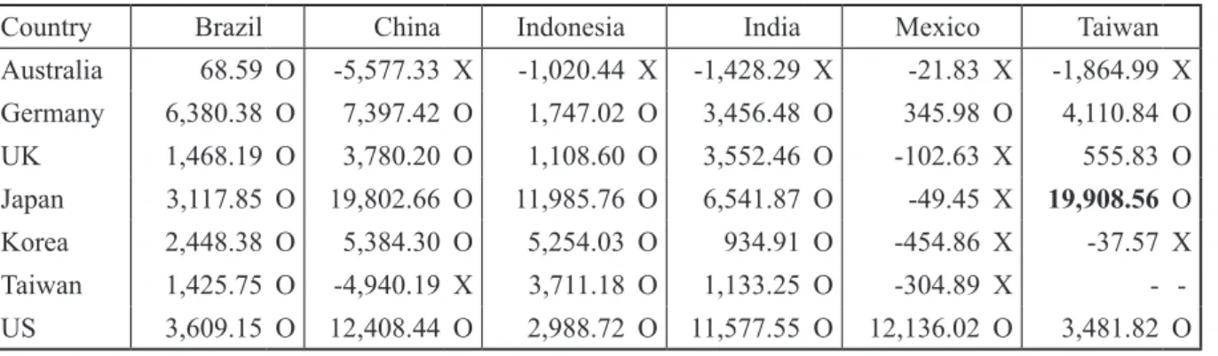
The results for net pollution exports in 2009 are shown in Table 1. In the table, an “O”
indicates that country s (shown on the first row) is the pollution haven of country r; on the other hand, an “X” indicates that r has been the pollution haven of s. As shown in Table 1, the largest net pollution export is that from Taiwan to Japan, which amounts to 19,908.56 thousand tones CO2e.
The most striking results are that for Australia.
Our results reveal that it has been the haven for most developing economies, and the reason is
Table 1. Net CO2e Exports in 2009 (by authors)
Country Brazil China Indonesia India Mexico Taiwan
Australia 68.59 O -5,577.33 X -1,020.44 X -1,428.29 X -21.83 X -1,864.99 X Germany 6,380.38 O 7,397.42 O 1,747.02 O 3,456.48 O 345.98 O 4,110.84 O UK 1,468.19 O 3,780.20 O 1,108.60 O 3,552.46 O -102.63 X 555.83 O Japan 3,117.85 O 19,802.66 O 11,985.76 O 6,541.87 O -49.45 X 19,908.56 O Korea 2,448.38 O 5,384.30 O 5,254.03 O 934.91 O -454.86 X -37.57 X Taiwan 1,425.75 O -4,940.19 X 3,711.18 O 1,133.25 O -304.89 X - - US 3,609.15 O 12,408.44 O 2,988.72 O 11,577.55 O 12,136.02 O 3,481.82 O
Unit: 1,000 tons.
that it exports a significant amount of agricultural products to these countries.
3.2 Relative CO
2e Emissions
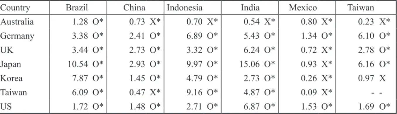
The results for relative pollution emissions are presented in Table 2. In the table, a value greater than 1 indicates that the source country is the pollution haven of the destination country.
The results of Table 2 reveal the same conclusions as that obtained from Table 1, which is quite obvious as both indexes are using exactly the same indicators of pollution emissions. However, recall that the largest number in Table 1 is that from Taiwan to Japan, but the largest number in Table 2 has been replaced by that from India to Japan (15.06). This is because that absolute quantity can change following the change of the scale of bilateral trade, while the ratio measure doesn’t.
Another interesting result shown in both tables is that for Mexico, our results indicate that many developed countries have been the haven of Mexico instead of the reverse. There might be two explanations to this. The first is that Mexico imports from more than exports to these countries;
and the second is that the trading relationships between Mexico and these countries are not as close as that between Mexico and the U.S., as revealed in the relatively small numbers from Mexico to these countries in Table 1.
3.3 Relative CO
2e Intensity
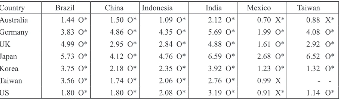
Finally, the results of relative pollution intensity are shown in Table 3. Different from the first two indexes which use gross trade statistics to calculate the index values, Index 3 takes into account the direct and indirect pollution emissions embodied in the production and consumption processes. This means not just the trade of final products but also the trade of intermediate goods has been included to measure the total pollution emissions3. Furthermore, Index 3 measures the relative intensity of the pollution emissions to avoid the possible misleading results from scale effects.
The results in Table 3 indicate that almost all developing economies examined are the pollution haven of the developed economies. Especially for Mexico, it is observed being the haven for only two of the developed countries using the previous
3 Bilateral embodied emission balances of Index 1 and 2 reflect a judgment as to whether the domestic country is a pollution haven for the foreign country with the assumption of that the domestic emission may increase through exports to the trading partner. However, Index 3 allocates the pollution content of imported goods to the final consumer. Even if the domestic country has the trade surplus with the trading partner, it could become a pollution haven after taking into account reflected back via third countries for consumption in the trading partner (trade of intermediate goods).
Table 2. Relative CO2e Emissions in 2009 (by authors)
Country Brazil China Indonesia India Mexico Taiwan
Australia 1.28 O* 0.73 X* 0.70 X* 0.54 X* 0.80 X* 0.23 X*
Germany 3.38 O* 2.41 O* 6.89 O* 5.43 O* 1.34 O* 6.10 O*
UK 3.44 O* 2.73 O* 3.32 O* 6.24 O* 0.72 X* 2.78 O*
Japan 10.54 O* 2.93 O* 9.97 O* 15.06 O* 0.93 X* 6.16 O*
Korea 7.87 O* 1.45 O* 4.79 O* 2.73 O* 0.26 X* 0.97 X
Taiwan 6.09 O* 0.47 X* 9.16 O* 4.87 O* 0.09 X* - -
US 1.72 O* 1.48 O* 2.71 O* 6.87 O* 1.53 O* 1.69 O*
* Indicates that the ratio is outside the range of 0.95 and 1.05. This is defined by authors as having an effect of the pollution haven where one country for the other country.
indexes but now becomes the haven for four out of the seven economies considered. The past several decades have witnessed that Mexico has become one of the major manufacturing bases of developed countries since its joining of the North America Free Trade Area (NAFTA). It is quite natural that companies of developed countries would move their factories to Mexico to take advantage of the agreement to either gain the market share in the North American market or establish supply chains to reduce production cost. Therefore, Mexico has gradually become a pollution haven of developed economies.
As for Taiwan, it is still the haven of most of the developed countries with Index 3, except for Australia. While the results of Index 1 and 2 show that Taiwan is not a haven for Korea, Index 3 does indicate that Taiwan is actually a haven of Korea in 2009. This means when taking into account the indirect effects of intermediates trade, the close tie between industries of the two countries have resulted in more and more exports from Taiwan to Korea which emit relatively more air pollution than the reverse, making Taiwan a pollution haven of Korea. The policy implication for Taiwan would, therefore, be to speed up the transformation of its industrial structure to limit the development of energy-intensive industries and, at the same time,
to promote the development of new and advanced technology with higher value added and energy efficiency.
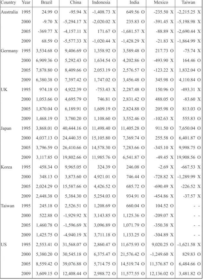
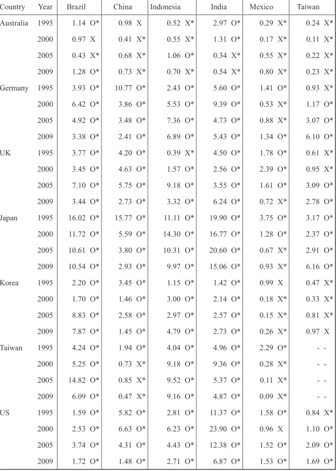
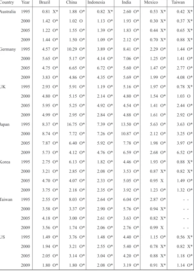
3.4 Trend Analysis
Table 4 to 6 present the trend of the three indexes. Table 4 shows that China has been the major haven of Japan and the U.S. from 1995 to 2009. However, there is a tendency that the positive balance for China towards being a haven is gradually diminishing. Similar situations can also be found for Indonesia and India. Taiwan, on the other hand, has revealed to become more and more a haven of Japan during the study period.
In addition, Taiwan reveals to gradually become a haven of Korea. Table 5 indicate similar trend as that found in Table 4. While from Table 6, we can see that although up to 2009 China is still the pollution haven of all the developed economies, it has gradually moved away from being the haven.
On the other hand, Indonesia and India are still the main haven of most of the developed economies.
For Taiwan, it was not a haven for Korea before 2005, but became the haven since, implying that Korea has surpassed Taiwan in production technology of many manufacturing industries after year 2005.
Table 3. Relative CO2e Intensity in 2009 (by authors)
Country Brazil China Indonesia India Mexico Taiwan
Australia 1.44 O* 1.50 O* 1.09 O* 2.12 O* 0.70 X* 0.88 X*
Germany 3.83 O* 4.86 O* 4.35 O* 5.69 O* 1.99 O* 4.08 O*
UK 4.99 O* 2.95 O* 2.84 O* 4.88 O* 1.61 O* 2.92 O*
Japan 5.73 O* 4.12 O* 4.76 O* 6.59 O* 2.68 O* 6.52 O*
Korea 3.75 O* 2.18 O* 2.35 O* 3.92 O* 1.23 O* 1.32 O*
Taiwan 3.56 O* 1.74 O* 2.06 O* 2.76 O* 0.99 X - -
US 1.80 O* 1.80 O* 2.08 O* 3.19 O* 0.91 X* 1.14 O*
* Indicates that the ratio is outside the range of 0.95 and 1.05.
Table 4. Trend of Net CO2e Exports (by authors)
Country Year Brazil China Indonesia India Mexico Taiwan
Australia 1995 24.99 O -95.94 X -1,408.73 X 649.56 O -235.50 X -2,215.25 X 2000 -9.70 X -5,294.17 X -2,020.02 X 235.83 O -391.45 X -5,198.98 X 2005 -369.77 X -4,157.11 X 171.67 O -1,681.57 X -88.89 X -2,690.44 X 2009 68.59 O -5,577.33 X -1,020.44 X -1,428.29 X -21.83 X -1,864.99 X Germany 1995 3,534.68 O 9,406.69 O 1,358.92 O 3,589.48 O 217.73 O -75.74 X 2000 6,909.36 O 5,292.43 O 1,634.54 O 4,202.86 O -493.90 X 164.46 O 2005 7,878.80 O 8,409.66 O 2,053.19 O 2,576.57 O -123.22 X 1,832.04 O 2009 6,380.38 O 7,397.42 O 1,747.02 O 3,456.48 O 345.98 O 4,110.84 O UK 1995 974.18 O 4,922.39 O -753.43 X 2,287.48 O 150.96 O -493.31 X 2000 1,053.66 O 4,695.79 O 746.81 O 2,831.42 O 488.05 O -83.60 X 2005 1,870.04 O 6,189.91 O 1,609.19 O 2,824.88 O 205.98 O 813.03 O 2009 1,468.19 O 3,780.20 O 1,108.60 O 3,552.46 O -102.63 X 555.83 O Japan 1995 3,868.01 O 40,444.16 O 11,498.40 O 11,405.28 O 911.50 O 7,650.04 O 2000 4,037.13 O 24,440.35 O 15,105.80 O 7,369.74 O 255.58 O 6,401.87 O 2005 3,796.59 O 26,410.66 O 14,578.30 O 7,283.66 O -345.10 X 9,998.75 O 2009 3,117.85 O 19,802.66 O 11,985.76 O 6,541.87 O -49.45 X 19,908.56 O Korea 1995 458.34 O 9,965.05 O 324.39 O 246.08 O -2.69 X -667.53 X 2000 348.13 O 3,873.60 O 4,921.01 O 746.44 O -728.82 X -1,289.99 X 2005 2,024.29 O 15,587.66 O 4,426.52 O 685.72 O -690.49 X -226.52 X 2009 2,448.38 O 5,384.30 O 5,254.03 O 934.91 O -454.86 X -37.57 X Taiwan 1995 245.18 O 2,526.51 O 1,208.69 O 660.04 O 104.52 O - -
2000 522.88 O -1,929.92 X 3,143.85 O 1,125.36 O -209.07 X - - 2005 1,460.78 O -1,596.69 X 3,096.89 O 1,071.79 O -350.38 X - - 2009 1,425.75 O -4,940.19 X 3,711.18 O 1,133.25 O -304.89 X - - US 1995 2,553.41 O 31,568.07 O 2,860.47 O 11,675.93 O 9,020.25 O -1,621.58 X
2000 5,380.20 O 30,545.18 O 6,375.47 O 21,576.42 O -1,249.60 X 829.83 O 2005 8,559.42 O 39,076.88 O 5,714.75 O 14,519.74 O 11,376.87 O 6,484.66 O 2009 3,609.15 O 12,408.44 O 2,988.72 O 11,577.55 O 12,136.02 O 3,481.82 O Unit: 1,000 tons.
Table 5. Trend of relative CO2e pollutions (by authors)
Country Year Brazil China Indonesia India Mexico Taiwan
Australia 1995 1.14 O* 0.98 X 0.52 X* 2.97 O* 0.29 X* 0.24 X*
2000 0.97 X 0.41 X* 0.55 X* 1.31 O* 0.17 X* 0.11 X*
2005 0.43 X* 0.68 X* 1.06 O* 0.34 X* 0.55 X* 0.22 X*
2009 1.28 O* 0.73 X* 0.70 X* 0.54 X* 0.80 X* 0.23 X*
Germany 1995 3.93 O* 10.77 O* 2.43 O* 5.60 O* 1.41 O* 0.93 X*
2000 6.42 O* 3.86 O* 5.53 O* 9.39 O* 0.53 X* 1.17 O*
2005 4.92 O* 3.48 O* 7.36 O* 4.73 O* 0.88 X* 3.07 O*
2009 3.38 O* 2.41 O* 6.89 O* 5.43 O* 1.34 O* 6.10 O*
UK 1995 3.77 O* 4.20 O* 0.39 X* 4.50 O* 1.78 O* 0.61 X*
2000 3.45 O* 4.63 O* 1.57 O* 2.56 O* 2.39 O* 0.95 X*
2005 7.10 O* 5.75 O* 9.18 O* 3.55 O* 1.61 O* 3.09 O*
2009 3.44 O* 2.73 O* 3.32 O* 6.24 O* 0.72 X* 2.78 O*
Japan 1995 16.02 O* 15.77 O* 11.11 O* 19.90 O* 3.75 O* 3.17 O*
2000 11.72 O* 5.59 O* 14.30 O* 16.77 O* 1.28 O* 2.37 O*
2005 10.61 O* 3.80 O* 10.31 O* 20.60 O* 0.67 X* 2.91 O*
2009 10.54 O* 2.93 O* 9.97 O* 15.06 O* 0.93 X* 6.16 O*
Korea 1995 2.20 O* 3.45 O* 1.15 O* 1.42 O* 0.99 X 0.47 X*
2000 1.70 O* 1.46 O* 3.00 O* 2.14 O* 0.18 X* 0.33 X*
2005 8.83 O* 2.58 O* 2.97 O* 2.57 O* 0.15 X* 0.81 X*
2009 7.87 O* 1.45 O* 4.79 O* 2.73 O* 0.26 X* 0.97 X
Taiwan 1995 4.24 O* 1.94 O* 4.04 O* 4.96 O* 2.29 O* - -
2000 5.25 O* 0.73 X* 9.18 O* 9.36 O* 0.28 X* - -
2005 14.82 O* 0.85 X* 9.52 O* 5.37 O* 0.11 X* - -
2009 6.09 O* 0.47 X* 9.16 O* 4.87 O* 0.09 X* - -
US 1995 1.59 O* 5.82 O* 2.81 O* 11.37 O* 1.58 O* 0.84 X*
2000 2.53 O* 6.63 O* 6.23 O* 23.90 O* 0.96 X 1.10 O*
2005 3.74 O* 4.31 O* 4.43 O* 12.38 O* 1.52 O* 2.09 O*
2009 1.72 O* 1.48 O* 2.71 O* 6.87 O* 1.53 O* 1.69 O*
* Indicates that the ratio is outside the range of 0.95 and 1.05.
Table 6. Trend of relative CO2e intensity (by authors)
Country Year Brazil China Indonesia India Mexico Taiwan
Australia 1995 0.81 X* 1.88 O* 0.82 X* 2.60 O* 0.53 X* 0.42 X*
2000 1.42 O* 1.02 O 1.13 O* 1.93 O* 0.30 X* 0.37 X*
2005 1.22 O* 1.55 O* 1.39 O* 1.83 O* 0.44 X* 0.65 X*
2009 1.44 O* 1.50 O* 1.09 O* 2.12 O* 0.70 X* 0.88 X*
Germany 1995 4.57 O* 10.29 O* 3.89 O* 8.41 O* 2.29 O* 1.44 O*
2000 5.65 O* 5.17 O* 4.14 O* 7.06 O* 1.25 O* 1.41 O*
2005 4.75 O* 6.65 O* 6.72 O* 5.60 O* 1.47 O* 2.77 O*
2009 3.83 O* 4.86 O* 4.35 O* 5.69 O* 1.99 O* 4.08 O*
UK 1995 2.93 O* 5.91 O* 1.19 O* 5.16 O* 1.97 O* 0.78 X*
2000 4.80 O* 5.15 O* 2.14 O* 4.80 O* 1.54 O* 1.03 O 2005 5.95 O* 5.25 O* 4.92 O* 4.54 O* 1.41 O* 2.44 O*
2009 4.99 O* 2.95 O* 2.84 O* 4.88 O* 1.61 O* 2.92 O*
Japan 1995 8.37 O* 16.75 O* 7.39 O* 13.50 O* 5.63 O* 3.63 O*
2000 8.74 O* 7.72 O* 7.26 O* 10.87 O* 2.12 O* 3.25 O*
2005 7.87 O* 6.40 O* 5.92 O* 7.78 O* 1.98 O* 3.97 O*
2009 5.73 O* 4.12 O* 4.76 O* 6.59 O* 2.68 O* 6.52 O*
Korea 1995 2.75 O* 6.13 O* 1.82 O* 4.46 O* 1.93 O* 0.88 X*
2000 3.21 O* 2.85 O* 2.08 O* 3.53 O* 0.87 X* 0.82 X*
2005 4.70 O* 4.07 O* 2.33 O* 5.05 O* 0.95 X 1.49 O*
2009 3.75 O* 2.18 O* 2.35 O* 3.92 O* 1.23 O* 1.32 O*
Taiwan 1995 2.55 O* 8.03 O* 2.64 O* 6.04 O* 2.87 O* - -
2000 3.58 O* 3.37 O* 2.90 O* 5.76 O* 0.94 X* - -
2005 4.18 O* 3.00 O* 2.61 O* 3.63 O* 0.82 X* - -
2009 3.56 O* 1.74 O* 2.06 O* 2.76 O* 0.99 X - -
US 1995 1.49 O* 3.76 O* 1.48 O* 4.40 O* 1.15 O* 0.56 X*
2000 1.94 O* 3.21 O* 2.55 O* 5.40 O* 0.78 X* 0.82 X*
2005 2.05 O* 3.14 O* 3.04 O* 4.20 O* 0.88 X* 1.18 O*
2009 1.80 O* 1.80 O* 2.08 O* 3.19 O* 0.91 X* 1.14 O*
* Indicates that the ratio is outside the range of 0.95 and 1.05.
4. Concluding Remarks
From the viewpoint of global value chain, one of the questions one would like to ask might be that whether the developing economies have constantly played the role of producing goods that make use of their abundant environmental resources and export the goods to developed economies, making developing economies the pollution haven of developed economies? The growing importance of global intermediates trade provides the direction of research on this important issue that both direct and indirect pollution should all be taken into consideration in order to correctly identify those economies that are haven of other economies. This present paper uses three indexes to examine which economies have been the pollution havens of other countries between 1995 and 2009. Although we comprehensively analyzed all 40 economies covered in the World Input- Output Database, we select only some of them to present the results, such as India, Indonesia, China, Brazil, and Mexico. We found that China has been the major haven of Japan and the U.S.
from 1995 to 2009. However, there is a tendency that the positive balance for China towards being a haven is gradually diminishing. Similar situations can also be found for Indonesia and India. For Taiwan, it was not a haven for Korea before 2005, but became the haven since, implying that Korea has surpassed Taiwan in production technology of many manufacturing industries after year 2005.
This result is a warning sign for Taiwan and the policy implication for Taiwan would be to speed up the transformation of its industrial structure to limit the development of energy-intensive industries and, at the same time, to promote the development of new and advanced technology with higher value added and energy efficiency.
Since the lack of input-output data in constant prices and price indexes for each country-industry, this paper adopts World Input-Output Tables in current prices to estimate the pollution emission.
Bias in the accounting of carbon content may occur as a result of fluctuations in commodity prices.
References
Aichele, R. and G. Felbermayr, 2015. “Kyoto and carbon leakage: An empirical analysis of the carbon content of bilateral trade,” Review of Economics and Statistics, 97(1): 104-115.
Al-Mulali, U., B. Saboori and I. Ozturk, 2015.
“Investigating the environmental Kuznets curve hypothesis in Vietnam,” Energy Policy, 76: 123-31.
Andrew, R., G. P. Peters and J. Lennox, 2009.
“Approximation and regional aggregation in multi-regional input–output analysis for national carbon footprint accounting,”
Economic Systems Research, 21(3): 311-335.
Antimiani, A., V. Costantini, C. Martini, L.
Salvatici and M. C. Tommasino, 2013.
“Assessing alternative solutions to carbon leakage,” Energy Economics, 36: 299-311.
Baldwin, R. and J. Lopez-Gonzalez, 2015.
“Supply-chain trade: A portrait of global patterns and several testable hypotheses,” The World Economy, 38(11): 1682-721.
Conrad, K., 2005. “Locational competition under environmental regulation when input prices and productivity differ,” Annals of Regional Science, 39(2): 273-295.
Copeland, B. R. and M. S. Taylor, 1994. “'North- South trade and the environment,” The Quarterly Journal of Economics, 109(3): 755- 87.
Dietzenbacher, E. and K. Mukhopadhyay, 2007.
“An empirical examination of the pollution haven hypothesis for India: Towards a green Leontief paradox?” Environmental and Resource Economics, 36(4): 427-49.
Eskeland, G. S. and A. E. Harrison, 2003. “Moving to greener pastures? Multinationals and the pollution haven hypothesis,” Journal of Development Economics, 70: 1-23.
Hertwich, E. G. and G. P. Peters, 2009. “Carbon footprint of nations: a global, trade-linked analysis,” Environmental Science and Technology, 43(16): 6414-6420.
IPCC, 2014. Climate Change 2014: Mitigation of Climate Change. Contribution of Working Group III to the Fifth Assessment Report of the Intergovernmental Panel on Climate Change. [Edenhofer, O., R. Pichs-Madruga, Y. Sokona, E. Farahani, S. Kadner, K.
Seyboth, A. Adler, I. Baum, S. Brunner, P.
Eickemeier, B. Kriemann, J. Savolainen, S.
Schlömer, C. von Stechow, T. Zwickel and J.C.
Minx (eds.)]. Cambridge University Press, Cambridge, UK and New York, NY, USA.
Johnson, R. C. and G, Noguera, 2012. “Accounting for intermediates: production sharing and trade in value added,” Journal of international Economics, 86(2): 224-36.
Kheder, S. B. and N. Zugravu-Soilita, 2008. “the pollution haven hypothesis: a geographic economy model in a comparative study,”
FEEM Working Paper No. 73.
Kuik, O. and R. Gerlagh, 2003. “Trade liberalization and carbon leakage,” The Energy Journal, 24(3): 97-120.
Lin, S. M., H. C. Yang and J. X. Lin, 2017. “A cross-country comparison of responsibility sharing in international carbon emissions,”
Taiwan Journal of Applied Economics, 101:
67-108.
Liu, X. and C. Wang, 2009. “Quantitative analysis of CO2 embodiment in international trade: an overview of emerging literatures,” Frontiers of Environmental Science and Engineering in China, 3(1): 12-19.
López, L. A., G. Arce and J. E. Zafrilla, 2013.
“Parcelling virtual carbon in the pollution haven hypothesis,” Energy Economics, 39:
177-86.
Peters, G. P., 2008. “From production-based to consumption-based national emission inventories,” Ecological Economics, 65(1):
13-23.
Peters, G. and C. Solli, 2010. Global Carbon Footprints: Methods and Import and Export Corrected Results from the Nordic Countries in Global Carbon Footprint Studies. Copenhagen, Norden: The Nordic Council and Nordic Council of Ministers.
Ricardo, D., 1891. Principles of political economy and taxation, G Bell and Sons, London.
Sato, M., 2014. “Embodied carbon in trade: a survey of the empirical literature,” Journal of economic surveys, 28(5): 831-861.
Su, B. and B. Ang, 2014. “Input-output analysis of CO2 emissions embodied in trade: A multiregion model for China,” Appled Energy, 114: 377-384.
Su, B., B. Ang and M. Low, 2013. “Input-output analysis of CO2 emissions embodied in trade and the driving forces: Processing and normal exports,” Ecological Economics, 88: 119-125.
Timmer, M. P., E. Dietzenbacher, B. Los, R.
Stehrer and G. J. Vries, 2015. “An illustrated user guide to the world input–output database:
the case of global automotive production,”
Review of International Economics, 23(3):
575-605.
Walter, I. and J. L. Ugelow, 1979. “Environmental
policies in developing countries,” Ambio, 8(2/3): 102-109.
Wang, Z., S. J.Wei, X. Yu and K. Zhu, 2017.
“Characterizing global and regional manufacturing value chains: Stable and evolving features,” Working Papers, h t t p / / d a g l i a n o . u n i m i . i t / w p - c o n t e n t / uploads/2017/01/WP2017_419.pdf.
Wiedmann, T. and J. Minx, 2008. A Definition of ‘Carbon Footprint’. In C. Pertsova (ed.), Ecological Economics Research Trends (pp. 1-11). Hauppauge, NY: Nova Science Publishers.
Zhang, Z., Y. Zhao, B. Su, Y. Zhang, S. Wang, Y.
Liu and H. Li, 2017. “Embodied carbon in China’s foreign trade: An online SCI-E and SSCI based literature review,” Renewable and Sustainable Energy Reviews, 68(1): 492-510.
Zhang, Z., J. E. Guo and G. J. Hewings, 2014.
“The effects of direct trade within china on regional and national CO2 emissions,” Energy Economics, 46: 161-175.
Zhang, Z., K. Zhu and G. J. Hewings, 2017. “A multi-regional input–output analysis of the pollution haven hypothesis from the perspective of global production fragmentation,”
Energy Economics, 64: 13-23.
從跨國生產及消費之碳含量檢視汙染避難所假說 是否成立
林晉勗
1曾琳芝
2張桂鳳
3*林師模
4摘 要
本研究以歐盟所編製的多國投入產出資料庫中,1995~2009年之多國投入產出表及三種空氣汙
染排放資料,從多國產業間互相關聯的角度,分析了各國各產業與生產及消費活動相關之汙染排放 含量,再進一步以所估算之數據檢視環境經濟學中之「汙染避難所假說」是否仍然普遍成立。本研 究以三種不同指標檢視汙染避難所假說是否成立,一是以進出口額為基礎,為多數傳統相關文獻的 計算方式;二是以進出口的相對比率為基礎;三則是結合附加價值貿易觀點,將附加價值貿易模型 中之附加價值向量轉換為空氣汙染排放係數向量,以計算出為了滿足其他國最終需要,本國各產業 生產時所導致的空氣汙染排放含量,以及為滿足本國最終需要,其他國家生產時所造成的空氣汙染 排放含量。本研究之結果發現,開發中國家之印度、印尼、中國大陸、巴西、墨西哥以三種指標檢 視,幾乎都是已開發國家的汙染避難所,而臺灣則是日本及美國的避難所。
關鍵詞:汙染避難所,多國投入產出分析,附加價值貿易,空氣汙染含量
收到日期: 2020年01月10日 修正日期: 2020年04月28日 接受日期: 2020年05月04日
1 中原大學國際經營與貿易學系 副教授
2 中原大學國際經營與貿易學系 碩士
3 中原大學商學博士學位學程 博士候選人
4 中原大學國際經營與貿易學系 特聘教授
*通訊作者電話: 03-2655222, E-mail: [email protected]