IEEE 802.15.4協定下能量收集無線感測網路之效能分析

(1)

國立臺灣大學電機資訊學院資訊工程學研究所碩士論文

Graduate Institute of Computer Science and Information Engineering College of Electrical Engineering and Computer Science

National Taiwan University Master Thesis

IEEE 802.15.4 協定下能量收集無線感測網路之效能分析 Modeling and Analysis of Energy Harvesting Sensor Nodes in

IEEE 802.15.4 Protocols

陳育旋 Yu-Hsuan Chen

指導教授：逄愛君博士

Advisor: Ai-Chun Pang, Ph.D.

(2)

謝

因為有許多人的幫忙，這篇論文才得以完成。

首先要感謝的是我的指導教授逄愛君老師，從我大四確定要進實驗室後，老師在研究以及生活上都給予了許多的協助，包含教導我做研究的方式和應有的態度、讓不是博士生的我遠赴紐西蘭做半年的研究、

以及安排我畢業後的出路，我對老師只有心中滿滿的感激。再來是我在紐西蘭做研究時的兩位教授 Winston 老師和 Bryan 老師，除了給我全額的獎學金，讓我在經濟上沒有顧慮外，老師們總是很關心我的適應狀況，而每週兩次的討論也會鼓勵我用很生硬的英文和大家分享我的研究成果，並適時的給予回應，在我回台灣後，還是定期和老師們書信往返，並且每週一次討論進度，希望我們之後的研究也可以順利，

最謝謝老師們的事情是，他們讓我相信，我的想法也可以很有價值。

再來是謝謝實驗室的淵耀學長、小泉學長、彥儒學長、清智學長和詩梵學姐在研究上的協助，還有不時的和大家聊天，讓實驗室的生活豐富了起來，也特別感謝學長姐在口試前兩天幫我們預演了四個小時。

再來謝謝我在紐西蘭的朋友們 Hang、Liang、Gloria、Alex、Deepak、

Michael、David 和 Abigail，大家中午總是圍在實驗室外的桌子吃自己帶來的午餐，聊一聊研究和生活中的趣事，讓我增長了不少對於國外和博士生活的見聞。最後要感謝我家人和小至對我的支持和幫助，讓我可以專心的完成這篇論文。

做研究就像一趟沒有終點的旅程，途中所見的風景就是最大的收穫。由衷的感謝這一路上幫助過我的所有人，謝謝。

(3)

中文要

在物聯網中，裝置的大小限制了本身能夠儲存的電量，使得網路的壽命受到影響，而藉由能量收集，讓裝置能夠自行充電，被視為一種延長網路壽命的方式。但是因為環境的影響，有別於以往用電池供電的方式，能量收集的電量大小會隨著時間變動，進而影響無線感測網路的運作，因此，以能量收集為供電方式的無線感測網路的效能需要被重新評估。在這篇論文中，我們嘗試用模型去描述使用能量採集來充電、並採用 IEEE 802.15.4 標準下的分槽式載波感測多重存取 / 碰撞避免 (CSMA/CA) 為 MAC 協定的裝置行為，並以平均充電時間、延遲和吞吐率做為效能評估的標準，我們提出的馬可夫模型成功的描述了通道競爭和充電的過程，並且比較使用不同的能量收集技術 (例如太陽能、振動能量收集等) 的裝置效能。模型會藉由模擬進行驗證，而分析出的吞吐率結果和模擬結果的誤差不會超過 6%。

關鍵字：物聯網、能量收集、IEEE 802.15.4 標準、分槽式載波感測多重存取 / 碰撞避免、馬可夫模型

(4)

Abstract

In the Internet of Things (IoT), the size constraint of those small and embedded devices limits the network lifetime because limited energy can be stored on these devices. In recent years, energy harvesting technology has attracted increasing attention, due to its ability to extend the network lifetime significantly. However, the performance of IoT devices powered by energy harvesting sources has not been fully analyzed and understood. In this paper, we model the energy harvesting process in IoT devices using slotted Car- rier Sense Multiple Access with Collision Avoidance (CSMA /CA) mechanism of IEEE 802.15.4 standard, and analyze the performance in terms of charging time, throughput and delay. Our new model successfully integrates the energy harvesting process and binary backoff process through a unified Markov chain model. Finally, the new model is validated by simulation and the throughput errors between simulation and analytical model are no more than 6%. We demonstrate the application of the model with different energy harvesting rate corresponding to different sources such as solar and vibration energy harvesters.

Keywords : Internet of Things, Energy Harvesting, IEEE 802.15.4 standard, CSMA/CA, Markov chain

(5)

List of Figures

1.1 Charging cycles of energy harvesting devices . . . 2

3.1 Slotted CSMA/CA mechanism with energy harvesting . . . 7

4.1 Markov model . . . 9

5.1 The assumption of each energy harvester in the simulation . . . 24

5.2 The charging time ratio derived from the simulation (sim) and analytical model (ana) under different parameter setting. The parameter E_max = 30, q₀ = 0.3, m₀ = 3 and m = 4 . . . . 26

5.3 The average throughput derived from the simulation (sim) and analytical model (ana) under different parameter setting. The parameter E_max = 30, q0 = 0.3, m0 = 3 and m = 4 . . . . 28

5.4 The average delay derived from the simulation(sim) and analytical model(ana) under different parameter setting. The parameter E_max = 30, q₀ = 0.3, m₀ = 3 and m = 4 . . . . 30

5.5 The performance with different value of E_min(m = 2, 3, 4, 5). The pa- rameter E_max= 30, N = 20, L = 7, q₀ = 0.3, and m₀ = 3 . . . 31

5.6 The performance with different value of E_max. The parameter N = 20, L = 7, q₀ = 0.3, m₀ = 3 and m = 4 . . . . 33

(8)

List of Tables

4.1 Symbols used to describe the System Model . . . 10

5.1 energy harvesting rate with 10cm² or 10cm³ harvesting material . . . 23

(9)

Chapter 1 Introduction

The uses of Internet of Things(IoT) appears in a range of different domains [1] such as structural health monitoring, animal tracking and environmental surveillance. Despite the ubiquitous deployment of IoT devices, one prevailing problem with the network is the limited energy stored on each device, which can suspend the network operation without notice. Since most sensing devices are small and embedded, the energy stored in each device is limited. How to assure that each device can harvest sufficient energy for continuous operation is an important issue.

Replenishing the energy source by replacing batteries is a way to extend the network lifetime. However, in most applications it is difficult perhaps infeasible to replace the batteries because of the physical and environmental constraints. To deal with this problem, energy harvesting for IoT devices have emerged as a promising technique to prolong the network lifetime.

Energy harvesting is a technique that can make the device harvest the ambient energy by itself, which has emerged as a prominent research topic after the use of IoT appears. It can be applied in many areas. For example, we install the solar panel on the solar vehicle, so the vehicle can be powered completely by direct solar energy. In body area networks, we put the thermoelectric energy harvesting material in the self-sustaining body sensor, and the material can generate power from the difference in temperature.

Although powering IoT devices by energy harvesting technology is one of the solutions to the limited available energy, the energy availability is not always assured. In wireless network, devices sense the channel and do backoffs to alleviate the channel contention, and

(10)

Figure 1.1: Charging cycles of energy harvesting devices

awake for a short period of time after harvesting energy. In most of the time, sensing devices cannot operate and is harvesting the energy, so the desired network performance can no longer achieved.

As illustrated in Fig. 1.1 [2], in wireless sensor networks, the energy characteristics of a node powered by energy harvesting is different from that of a node powered by batteries.

For an energy harvesting node, it cannot operate until the harvested energy is accumulated to a certain level. During the node operation, if the node exhausts the energy, it stops the operation to be recharged. Since the charging cycle can be repeated, the energy harvesting device can work for a very long time without replenishing the energy source manually, but the performance is affected by the energy harvesting time.

To achieve adequate, the energy-constrained condition should be considered. Conse- quently, the existing Multiple Access Protocol(MAC) will not be valid under such condition. Different MAC protocols for IoT with energy harvesting are analyzed through experiments, and the result shows that the energy harvesting process directly affects the performance of network throughput via the MAC protocols [3, 4].

In this paper, we try to find out how the energy harvesting process affect the network performance. We consider the slotted Carrier Sense Multiple Access with Collision Avoid- ance (CSMA/CA) mechanism in IEEE 802.15.4 standard as the MAC protocol. For sim- plicity, we assume that the network topology is a single hop network with a star topology.

We derive the expressions for charging time ratio, throughput and delay from the model,

(11)

and validate the model through simulations. Through the proposed model, we characterize the effect of energy replenishment process on the performance of IEEE 802.15.4 MAC protocol, and show the effect of energy harvesting rate on the performance.

The remainder of this paper is structured as follows. In Chapter II, we review related works. In Chapter III, we briefly describe the slotted CSMA/CA mechanism of the IEEE 802.15.4 standard, and explain how it interacts with the energy harvesting process.

In Chapter IV, we propose a Markov chain model of the slotted CSMA/CA mechanism integrated with the energy harvesting process. In Chapter V, the model is validated by simulation and we compare the network performance with different energy harvesting rates.

Chapter VI concludes the paper.

The contributions of this paper are: (i) a new model that integrates energy harvesting with slotted CSMA/CA mechanism of IEEE 802.15.4 standard within a unified Markov model, (ii) the energy harvesting process and the backoff process can take on different parameters, (iii) the energy consumption during binary backoff, clear channel assessment and packet transmission are necessarily distinct, and (iiii) we can successfully explain how the energy harvesting process affects the network performance. Contributions (ii) and (iii) relaxes assumptions in existing models and reflects the real-world IoT devices behaviour more closely.

(12)

Chapter 2 Related Work

2.1 IEEE 802.15.4 protocol

The IEEE 802.15.4 MAC protocol is widely adopted in IoT for example, 6LoWPAN, ZigBee and WirelessHART. It specifies the semantics for low-cost and low-power sensor networks operation. One of the access mechanisms specified by IEEE 802.15.4 standard is slotted Carrier Sense Multiple Access with Collision Avoidance (CSMA/CA) mechanism, and several simulation-based studies e.g., [5–9], analyze this protocol through Markov chain models. Most of the studies are based on Bianchi’s work [10], which uses a bi- dimensional Markov chain model for IEEE 802.11 DCF.

The model developed in [6] fails to match the result, since they make the same assumption as [10] for the 802.11. The model in [5] correct this problem, but they derive the wrong probability for the channel sensing. [7] assumes that, in IEEE 802.15.4 standard, the probabilities to start channel sensing for the different devices should be independent.

In [8], a packet’s retry limit is considere. In [9], in addition to the packet’s retry limit, they also consider the superframe structure of the 802.15.4 protocol. The Markov models that appear in [7–9] successfully predict the performance of the 802.15.4 protocol. How- ever, these models assume that sensing devices have unlimited power, which limits the applicability of the model and simulation result in practical settings.

2.2 Energy Harvesting process

Some studies e.g., [11–14], have modelled the energy replenishment (recharging) pro- cess with varying degrees of success. A favoured approach for modelling the energy replenishment is the Markovian energy model which appears in [11], [12] and [13]. The

(13)

model in [11] assumes that the packet arrival and energy replenishment are both memory- less Poisson process, and the energy state transition follows the birth and death process. A further assumption is that packet transmissions are not interrupted by the energy replenishment, which is not valid in the real energy harvesting environment, but yields insights into how throughput is affected by energy harvesting process.

To relate more realistic energy harvesting, the authors in [12] use a stochastic process to model solar and piezoelectric energy sources. The work in [12] is devoted to deriving models for optimizing energy harvesting with less attention to the interactions between protocol and energy harvesting, thus the approach therein is different.

In [13], the energy model is modelled as a Bernoulli process and is unified with the slotted CSMA/CA mechanism of the IEEE 802.11 standard. In their model, the packet length and the backoff counter freezing time are not modelled, and the energy consumption during the channel sensing state is ignored, which does not reflect changes in residual energy correctly.

(14)

Chapter 3 Overview of IEEE 802.15.4 Slotted CS- MA/CA

In this chapter, we briefly explain the slotted CSMA/CA mechanism of the IEEE 802.15.4 standard [15], and highlight the interaction with an energy harvesting process.

In the slotted CSMA/CA mechanism, there are three important variables [16] :

1. The Number of Backoffs (NB) is the number of times the algorithm has performed binary backoff before the packet transmission attempt. The value is initialized to 0 for a new transmission attempt.

2. The Contention Window (CW) is the number of backoff periods that the channel is required to be sensed idle before the transmission attempt. The value of CW is initialized to CW₀. If the node operation is in the Japanese 950 MHz band, CW₀ shall be set to 1; otherwise, CW₀shall be set to 2.

3. The Backoff Exponent (BE) controls the number of backoff periods that the algo- rithm needs to backoff before sensing the channel. The number of backoff periods is a random variable between [0, 2^BE-1].

Figure 3.1 is the flow chart of the slotted CSMA/CA mechanism with energy har- vesting. First, the variables NB and CW are initialized to 0 and 2 respectively, while BE is initialized to min (2, macMinBE) or macMinBE depending on the battery life exten- sion(BLE). When BLE value is true, the MAC sublayer limits the random backoff exponent to ensure that the backoff duration, CCA and packet transmission is completed quickly (hence conserving energy). (Step 1). Next, the algorithm counts down a number of backoff periods which is randomly selected from [0, 2^BE-1] (Step 2). After counting

(15)

Figure 3.1: Slotted CSMA/CA mechanism with energy harvesting

down to 0, the algorithm performs Clear Channel Assessment (CCA) to check if the chan- nel is idle (Step 3). If the channel is idle, CW is decreased by 1 (Step 4). If CW is equal to 0, the packet can be transmitted (Step 5), or the CCA is repeated. If the channel is sensed busy, N B is increased by 1, CW is reinitialized and BE is reinitialized to min(BE+1, macMaxBE) (Step 6). If macMaxCSMABackoffs is reached, the packet is discarded (Step 7); otherwise, the backoff process restarts.

In this paper, we assume the MAC layer checks the remaining energy of the device after the packet transmission or access failure and this is shown in the red shaded blocks in Fig. 3.1. If the energy is below a threshold denoted by E_min, the energy harvesting process starts, and the energy is replenished before a new packet transmission attempt.

(16)

Chapter 4 System Model

In this section, we integrate an energy harvesting process to the IEEE 802.15.4 slotted CSMA/CA mechanism to characterize the performance of a network of IoT devices powered by energy harvesting. We focus on a single hop star network, in which every device transmits packets to the personal area network (PAN) coordinator and receives an acknowledgement (ACK). In the model, we assume that each device has a supercapacitor to store energy, and the maximum energy capacity of the supercapacitor is Emaxunit.

During normal operation, defined as the MAC protocol in the following set of states:

{idle, backoff, channel sensing, packet transmission}, energy is decreased. After the packet transmission process (success or collision) is finished, the device checks its re- maining energy level. If the remaining energy is less than E_min units, the device halts operation and enters the energy harvesting process; otherwise, the device waits for a new packet arrival.

4.1 Energy harvesting process

Energy harvesting is the process by which ambient energy is captured and stored in the supercapacitor. We assume that the energy harvesting process follows the Poisson process to reflect the deployments of IoT in several sensor network scenarios such as structural health monitoring environments [17], bridge monitoring [18] and harvesting solar energy in situations whereby the solar irradiance is variable due to the passing of clouds [19]. The energy harvesting process stops when the energy level in the supercapacitor reaches E_max and the CSMA/CA mechanism restarts operation.

(17)

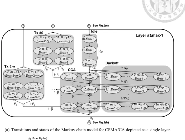
(a) Transitions and states of the Markov chain model for CSMA/CA depicted as a single layer.

(b) Transitions between adjacent CSMA/

CA backoff layers. This figure is con- nected to Fig. 4.1(a).

(c) Transitions and states of the energy harvesting sub-chain.

Figure 4.1: Markov model

(18)

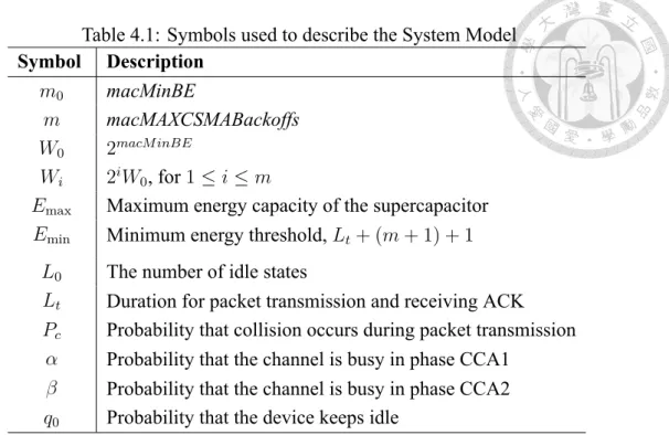
Table 4.1: Symbols used to describe the System Model Symbol Description

m₀ macMinBE

m macMAXCSMABackoffs W₀ 2^{macM inBE}

W_i 2ⁱW₀, for 1≤ i ≤ m

E_max Maximum energy capacity of the supercapacitor E_min Minimum energy threshold, L_t+ (m + 1) + 1

L₀ The number of idle states

L_t Duration for packet transmission and receiving ACK P_c Probability that collision occurs during packet transmission

α Probability that the channel is busy in phase CCA1 β Probability that the channel is busy in phase CCA2 q₀ Probability that the device keeps idle

4.2 State space of the Markov model

The Markov chain model for the IEEE 802.15.4 slotted CSMA/CA mechanism with energy harvesting is shown in Fig. 4.1. The state space is categorized into four sets of states and each set is characterized with different indices. Let e(t), f (t), h(t), s(t) and k(t) be stochastic processes representing the the backoff stage number, the state of the backoff counter, the residual energy level of a device, the energy harvested and the number of packets awaiting transmission at time t respectively. The tuple{δ(t), e(t), f(t), h(t)}

form the set of transmission states whereby δ(t) is the indicator process of a successful transmission or otherwise defined in Eq.(4.1). This set of states are grouped and labelled as “Tx #0” and “Tx #m” in Fig.4.1(a).

δ (t) =











−1 if transmission successful at time t

−2 if transmission unsuccessfull at time t

(4.1)

Transmission states {−1, i, j, s} and {−2, i, j, s} represent the successful and collided packet transmissions respectively with the indices bounded by i∈ [0, m], j ∈ [0, Lt− 1]

and s∈ [Emax− 2 − m − Lt, Emax− m − 3].

The backoff process is characterised by stochastic processes e(t), f (t) and h(t) and

(19)

the tuple{e(t), f(t), h(t)} denotes the set of backoff states and the set of CCA states (these sets are labelled as “Backoff” and “Idle” in Fig. 4.1(a). Backoff states{i, w, s}

are bounded by i ∈ [0, m], w ∈ [1, Wi− 1], in which i is the backoff stage, and w is the backoff counter. The first phase (CCA1) and the second phase (CCA2) of the CCA are denoted by states{i, 0, s} and {i, −1, s} , i ∈ [0, m] respectively.

The behaviour of an idle device waiting for a new packet arrival is modelled by k(t) and s(t), therefore the tuple{k(t), s(t)} denotes the set of idle states with the tuple de- fined in the range of{c, s}, c ∈ [0, L0− 1], s ∈ [0, Emax− 1]. Note that the degree of traffic saturation is regulated through the parameter L₀. Finally, the energy harvesting is governed by a single process s(t) with s∈ [0, Emax− 1] and it forms a sub-chain shown in Fig.4.1(c).

The variable Lt denotes the number of backoff periods for packet transmission and receiving ACK and it is expressed as L_t = L+t_ack+L_ack, where L is the number of backoff periods for packet transmission, t_ackis the idle period between the packet transmission and receiving ACK, and L_ackis the number of backoff periods for receiving ACK. Based on the 802.15.4 standard specifications [15] we set t_ack = 1 backoff period and L_ack = 2 backoff periods. Throughout this paper, we assume that the duration for successful packet transmission and the duration for collided packet transmission are identical.

Recall that the states s∈ [0, Emax− 1] are energy harvesting states with s representing the residual energy level of the device, and the energy harvesting is governed by a Poisson process with rate λ. The value of λ dictates the energy units harvested in a backoff period.

According to the energy consumption rates in different states, we assume that there is no energy consumption in backoff states [7]. In our model, idle states collectively consume one unit of energy, thus CCA1 and CCA2 together consume one unit energy, and each of the transmission state consumes one unit of energy. The value of E_min is the sum of the energy consumed during packet transmission, the total number of backoff stages, and the

(20)

In Fig. 4.1(c), the constant e is equal to E_min − 1. Table 4.1 lists the symbols and the meanings in the context of the Markov model.

4.3 State transitions

Our model in Fig. 4.1 is composed of layers, and these layers are linked to energy harvesting states. Each layer has the same structure in terms of states and transitions.

When a device terminates packet transmission and the remaining energy level s is greater than Emin, the device transits to the idle state in another layer with probability q0, or transits to the backoff state with probability 1−q0. But if s is less than E_minunit, the device transits to the energy harvesting state. For example, if the packet transmission is done in the state (−1, 0, Lt− 1, Emax− 2 − Lt) and (E_max− 2 − Lt) is greater than E_min, the state of the device transits to the idle state (0, (E_max− 2 − Lt)− 1) with probability q0.

The index of a layer models the remaining energy level of the device when in idle states and this index is an integer defined over the range of E_min − 1 to Emax − 1. In energy harvesting states, the permissible state transitions are shaded (green in Fig. 4.1(c)) and the sojourn time of energy harvesting states follows an exponential distribution.

Using simplified notation Pr{E} where E denotes a transition event of the MAC, the non-null state transition probabilities of the Markov chain are:

Pr{harvesting one unit of energy}

= P (s + 1|s) = e^λλ, for 0≤ s < Emax− 1, (4.3) Pr{transit to the first backoff stage from an idle state}

= P (0, w, s|L0, s)

= P (0, 0, s− 1|L0, s)

= 1− q0

W₀ , for 1≤ w < W0, (4.4)

(21)

Pr{the decrement of the backoff counter}

= P (i, w− 1, s|i, w, s)

= P (i, 0, s− 1|i, 1, s)

= 1, for 0≤ i ≤ m and 1 < w < W0, (4.5)

Pr{new backoff after channel sensed busy during CCA1 or CCA2 }

= P (i, w, s|i − 1, 0, s)

= P (i, 0, s− 1|i − 1, 0, s)

= α + (1− α)β

W_i , for 1≤ i ≤ m and 1 ≤ w < Wi, (4.6) Pr{channel is idle during CCA1 and CCA2 upon a successful packet transmission}

= P (−1, i, 0, s − 1|i, 0, s)

= (1− α)(1 − β)(1 − Pc), (4.7)

Pr{channel is idle during CCA1 and CCA2 after a collision}

= P (−2, i, 0, s − 1|i, 0, s)

= (1− α)(1 − β)Pc. (4.8)

The probability that the device is in the wait state (awaiting packet arrivals) or is charged after the transmission is denoted by Eq. (4.9) and Eq. (4.10) respectively. Therefore, the non-null transition probabilities are:

Pr{waiting state after a packet transmission}

= P (0, s− 1| − 1, i, Lt− 1, s)

= P (0, s− 1| − 2, i, Lt− 1, s) =











q₀, if s≥ Emin

0, if s < E_min

, (4.9)

(22)

Pr{energy harvesting after the packet transmission}

= P (s| − 1, i, Lt− 1, s)

= P (s| − 2, i, Lt− 1, s) =











0, if s≥ Emin

1, if s < E_min

. (4.10)

If the remaining energy level is below E_min, the device halts normal operation and the energy harvesting process starts. Subsequently, the probability that the device is in a wait state (awaiting packet arrival) or is charged after the access failure is given by Eq. (4.11) and Eq. (4.12). The device waits for a new packet arrival only if the remaining energy level is above E_min. Thus, the non-null transition probabilities are:

Pr{waiting state after an access failure}

= P (0, s− 1|m, 0, s)

=











q₀ × (α + (1 − α)β), if s ≥ Emin

0, if s < E_min

, (4.11)

Pr{energy harvesting after the access failure}

= P (s|m, 0, s) =











0, if s ≥ Emin

α + (1− α)β, if s < Emin

. (4.12)

4.4 Stationary distribution

The stationary distribution of the embedded Markov chain of Fig. 4.1 is a vector π.

For ease of presentation, we decompose the vector into four different states:

• idle states, the stationary probability is

π_c,s, c ∈ (0, L0− 1), s ∈ (Emin− 1, Emax− 1),

(23)

• backoff / CCA states, the stationary probability is

πi,w,s, i∈ (0, m), w ∈ (−1, Wi − 1),

• packet transmission states, the stationary probability is

π_−1,i,j,sand π_−2,i,j,s, i∈ (0, m), j ∈ (0, Lt− 1),

• energy harvesting states, the stationary probability is

π_s, s∈ (0, Emax− 1),

such that

π = (πc,s∪ πi,w,s∪ π−1,i,j,s∪ π−2,i,j,s∪ πs) .

Using this notation, the transition probabilities that appear earlier in Eq. (4.4) and Eq.

(4.5) are simplified to:

π_i,w,s+1 = W_i− w Wi

π_i,0,s, (4.13)

where w is from 1 to W_i − 1. Similarly, the transition probabilities in Eq. (4.6) are expressed as

π_i,0,s_−i = (α + (1− α)β)ⁱπ_0,0,s. (4.14)

Summing the state probabilities for a layer indexed by s (i.e. Eq. (4.4) - (4.8), Eq. (4.13) and Eq. (4.14)), we obtain the probability the Markov chain is in layer s:

L₀× π0,s+ π_0,0,s₋₁

2 (1− (2x)^m+1

1− 2x W₀ +1− x^m+1 1− x ) + (1− α)1− x^m+1

1− x π_0,0,s₋₁+ L_t(1− x^m+1)π_0,0,s₋₁

(24)

where x = α + (1− α)β.

From Eq. (4.15) we expand the expressions for π_0,sand π_0,0,s₋₁ and this yields:

π_0,s =











π_Emax−1

1−q0 , if s = E_max− 1

q0(Qa(s)+Qb(s))

1−q0 , otherwise

, (4.16)

and π0,0,s−1is given by:

π_0,0,s₋₁=











(1− q0)π_0,s, if s = E_max− 1 (1− q0)(Q_a(s) + Q_b(s) + π_0,s), otherwise

, (4.17)

where Qa(s) is the state transition probability to layer s due to the packet transmission and Q_b(s) is the state transition probability to s conditioned on access failure. Using Eq. (4.16) and Eq. (4.17), we establish the relationship between π_0,sand π_0,0,s₋₁which expresses the probability the Markov chain is in state s (Eq. (4.15)) as a function of π_0,s.

The derivation of Q_a(s) is as follows: we introduce the auxiliary variable r = (s + 1) + L_t, to denote the remaining energy level of the device during its successful CCA1 and CCA2. For r + 1 > E_max− 1, the corresponding Qa(s) is 0, while for r + 1≤ Emax− 1, we obtain Qa(s) as:

Q_a(s) =^∑ⁿ

i=(r+1)+0(1− α)(1 − β)πi−(r+1),0,r

=^∑ⁿ

i=(r+1)+0(1− α)(1 − β)xⁱ^−(r+1)π_0,0,i₋₁,

where (r + 1) and n = min (E_max− 1, (r + 1) + m) are the respective minimum and maximum index of layers that the state transition from these layers to state (0, s) after the packet transmission exists. This relationship is direct from Eq. (4.7) and Eq. (4.8).

(25)

Moreover, from Eq. (4.11), the expression for Q_b(s) is readily obtained as:

Q_b(s) =











0, if d > E_max− 1 x× πm,0,s+1, if d≤ Emax− 1

, (4.18)

where d = (s + 1) + m + 1, which is the index of the layer and the state transition from the layer to state (0, s) after an access failure. When d ≤ Emax− 1, the probability the Markov chain transits to state s can be rewritten as follows:

Qb(s) = x× πm,0,s+1 = x^m+1π0,0,d−1.

Now, we will derive the stationary distribution expressions for the energy harvesting states π_s, s ∈ (0, Emax− 1). Starting from the expressions in Eq. (4.3), Eq. (4.10) and Eq. (4.12), we have:

π_s=











R_a(s) + R_b(s), if s = 0

R_a(s) + R_b(s) + π_s₋₁, if 0 < s≤ Emin− 1 π_E_min₋₁, if E_min− 1 < s

(4.19)

where Ra(s) is the probability that the device starts energy harvesting process with re- maining energy level s after the packet transmission, and Rb(s) is the probability that the device starts energy harvesting process with remaining energy level s after the access failure.

The derivation of R_a(s) is similar to that of Q_a(s). Denote the remaining energy level of the device during its successful CCA1 and CCA2 by u such that u = s + L_t. When u + 1 > E_max− 1, the value of Ra(s) is 0. When u + 1 ≤ Emax− 1, the expression of R_a(s) is

(26)

where v = max(u + 1, E_min− 1) and k = min((u + 1) + m, Emax− 1) are the minimum and maximum index of those layers that can transit to state (s) after the access failure, respectively. The expression of R_b(s) is

R_b(s) =











0, if s + m + 1 < E_min− 1 0, if s + m + 1 > E_max− 1

x× πm,0,s, if E_max− 1 ≥ s + m + 1 ≥ Emin− 1

. (4.21)

When s + m + 1≥ Emin− 1, we can rewrite Rb(s) as

x× πm,0,s= x^m+1π_0,0,s+m

The probability of each state in Eq. (4.15) - (4.21) can be rewritten as a function of π0,0,s−1, s∈ (Emin−1, Emax−1). Given that we have derived the relations of π0,sand π_0,0,s₋₁, the sum of the stationary probability of Markov chain can further be expressed by π_0,E_max₋₁. We now derive the remaining unknowns α, β and P_cby considering the sojourn time of the states. Let P be the limiting probability of the Markov chain in Fig. 4.1. For CCA1 states, the limiting probability P_i,0,sand its relationship with π_i,0,sis given by:

P_i,0,s = lim

t→∞P_i,0,s(t) = π_i,0,sE(T_i,0,s)

∑

k∈Sπ_kE(T_k),

where T_kis the sojourn time of state k, and S presents a set of discrete states of the Markov chain. Because the sojourn time of each state in each layer is normalized to a unit backoff period, and the sojourn time of energy harvesting states depends only on the harvesting rate λ, the limiting probability of CCA1 states is readily expressed as a function of π0,Emax−1. Next, we introduce a probability τ that the device performs its CCA1 in a random back- off period, which is equal to the sum of the limiting probability of CCA1 states. Similar to [8], the value of τ is given by

τ =

Emax∑−2 s=Emin−2

1− x^m+1

1− x P_0,0,s. (4.22)

(27)

Now, we can derive the probabilities α, β and P_c. The conditional collision probability P_c is the probability that the collision occurs during packet transmission. In the slotted CSMA/CA mechanism, a collision occurs only if at least one of the remaining N − 1 devices start packet transmission in a same backoff period. Hence, Pcis

P_c= 1− (1 − τ)^N⁻¹, (4.23)

where N is the number of nodes.

The probabilities α and β are the probabilities that the channel is sensed busy during CCA1 and CCA2:

α = α₁+ α₂, (4.24)

where α1is the probability that the channel is sensed busy during CCA1 due to the packet transmission (the proof of (4.24) appears in [7] and [8].) Since the probability that a device starts to transmit a packet is τ (1− α)(1 − β), and 1 − (1 − τ)^N⁻¹ is the probability that at least one of the N− 1 remaining devices stay in CCA1 states, α1 is

α1 = L(1− (1 − τ)^N⁻¹)(1− α)(1 − β)

and α₂ is the probability that the channel is sensed busy during CCA1 due to ACK transmission, which is expressed as:

α2 = Lack

N τ (1− τ)^N⁻¹(1− α)(1 − β) (1− (1 − τ)^N)(1− α)(1 − β)

× (1 − (1 − τ)^N⁻¹)(1− α)(1 − β)

= L_ackN τ (1− τ)^N⁻¹

1− (1 − τ)^N (1− (1 − τ)^N⁻¹)(1− α)(1 − β),

(28)

transmitting the packet. The probability that the channel is sensed busy (denoted by β):

β = 1− (1 − τ)^N⁻¹+ N τ (1− τ)^N⁻¹

2− (1 − τ)^N + N τ (1− τ)^N⁻¹ . (4.25)

Further details about deriving the probabilities α, β and P_c appear in [7]. With the com- plete characterization of these transition probabilities, the model is solved numerically.

4.5 Expression of Charging Time Ratio, Throughput and Delay

In this section, we try to derive the expression of charging time, throughput and delay from the proposed model.

Charging time ratio is the ratio of the energy harvesting time to the device’s whole system time, and the whole system time is the energy harvesting time plus the CSMA/CA operation time. For example, if charging time ratio = 0.6, it means that in 10 minutes, the device will take 6 minutes to capture the ambient energy and take 4 minutes to perform the CSMA/CA operation. The average charging time ratio is derived by the following expression:

Charging time ratio(ana)

= energy harvesting time

energy harvesting time + CSMA/CA operation time

=

∑_E_max₋₁

s=0 π_sE(T_s)

∑

k∈Sπ_kE(T_k) ,

in which Tkis the sojourn time of state k, and S represents a set of discrete states of the Markov chain.

Next, we derive the average throughput. Similarly to [7], The average throughput from our analytical model is equal to:

Throughput(ana) = LN τ (1− τ)^N⁻¹(1− α)(1 − β)

(29)

where N τ (1− τ)^N⁻¹(1− α)(1 − β) is the probability that only one device is transmitting the packet.

The derivation of the average delay from the analytical model is similar to that in [8].

However, in our model, we assume that the packet is dropped if the collision or access failure occurs, so macMaxFrameRetries = 0.

(30)

Chapter 5 Model Validation

In this chapter, we validate the proposed model by simulation, and analyze the performance in terms of charging time, throughput and delay. The simulation is developed in Matlab.

5.1 Simulation Setup

The algorithm follows the pseudo code proposed in [7] and we extend it to accommo- date acknowledgements and the unsaturated traffic conditions. Because the device only changes state at the backoff period boundaries, we normalize the simulation step to one backoff period. The total simulation time is 10⁸ backoff periods.

For the probability q₀, we generate a uniform random number between 0 and 1. If the number is not bigger than q₀, the device remains idle, otherwise it starts the backoff process. The size of the backoff counter is a randomly chosen integer between 0 to 2^BE−1.

5.1.1 Expression of Charging Time Ratio, Throughput and Delay

The average charging time for each device is:

Charging time ratio(sim) = T_charging N× Tsimulation

where T_chargingdenotes the sum of devices’ energy harvesting time. The average throughput from the simulation is simply:

Throughput(sim) = ns× L T_simulation

(31)

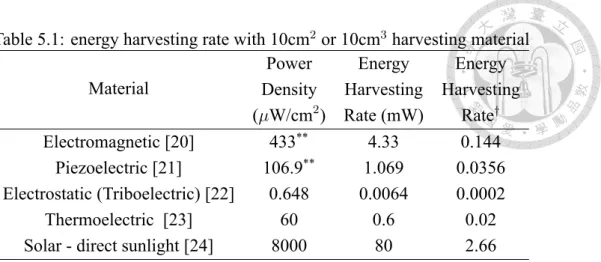
Table 5.1: energy harvesting rate with 10cm²or 10cm³harvesting material

Material

Power Energy Energy

Density Harvesting Harvesting (µW/cm²) Rate (mW) Rate^†

Electromagnetic [20] 433^** 4.33 0.144

Piezoelectric [21] 106.9^** 1.069 0.0356 Electrostatic (Triboelectric) [22] 0.648 0.0064 0.0002

Thermoelectric [23] 60 0.6 0.02

Solar - direct sunlight [24] 8000 80 2.66

†the energy units harvested in a backoff period

**unit is µW/cm³

where n_s denotes the number of successfully transmitted packets, and T_simulation refers to the total simulation time. The unit of the packet length L and the unit of simulation time are both a backoff period.

Next, we derive the average delay. We define the average delay of a packet as the time from the first attempt of backoff, until the time when the ACK is received. Consistent with the analytical model, we do not consider the delay of discarded packets due to the collision or access failure. The expression of the average delay is as follows:

Delay(sim) = T_delay n_s × T

where T_delay denotes the sum of packets’ delay while T is the length of the backoff pe- riod. According to IEEE 802.15.4 standard [15], a backoff period is 20 symbols long (aUnitBackoffPeriod), and 1 symbol is 4 bits. For a typical bit rate of 250kbps, T is

80bits

250kbps = 0.32ms.

5.1.2 Setting of the energy harvesting rate

The energy harvesting rates from different energy harvesting technologies with di-

(32)

0 7 14 21 28 35 42 49 56 63 70 77 84 Time(backoff period)

0 0.5 1 1.5

Harvested Energy(unit)

(a) Electromagnetic energy harvester

0 28 56 84

Time(backoff period) 0

0.5 1 1.5

(b) Piezoelectric energy harvester

0 10 20 30 40 50 60 70 80

Time(backoff period) 1

1.5 2 2.5 3

(c) Solar energy harvester

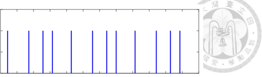
Figure 5.1: The assumption of each energy harvester in the simulation

In [21], the energy is harvested using piezoelectric bimorph/magnet compsites and an AC power line. When the power is switched on, the AC magnetic field interacts with the mag- netization of the magnet inciting the piezoelectric cantilever. In [22], they implement the electrodes, diode ladder circuit and a energy harvesting circuit on skirt paddles. Due to the triboelectric effect, these paddles generate electrostatic energy when brushed rapidly against each other. In [23], they wear the 9cm² thermoelectric energy harvester on the wrist. Using the temperature difference between the skin and ambient temperature, the thermoelectric energy is generated. The maximum generated power is about 60µW/cm² indoors and about 600µW/cm² at a temperature of 0^°C. In [24], the National Institute of

(33)

Water and Atmospheric Research(NIWA) conducts the SolarView calculation for a year in Kelburn, Wellington. The lowest harvested Solar Energy during daylight is 80mW.

In this paper, we assume that the energy consumption rate for packet transmission is 30mW [8], and the actual length of a backoff period is 0.32ms. Using this relationship, the energy harvesting rate from mW is easily converted to the energy unit per backoff period and this is used to tabulate the harvesting rate in the fourth column of Table 5.1. In the paper, we choose the harvesting rate λ = 2.5, 0.14, 0.035 as the simulation parameter, in which the rate = 2.5 is close to the rate given by outdoor solar energy harvesters, the rate

= 0.14 is close to the rate given by electromagnetic energy harvesters, and rate = 0.035 is close to the rate given by piezoelectric energy harvesters.

In the simulation, we assume that each energy harvesting process follows different distribution. Since electromagnetic energy and piezoelectric energy are both the energy of vibrations, we suppose that the vibration occurs once in each cycle time, and we can harvest 1 unit of the energy when the vibration occurs. As shown in Fig. 5.1(a), for the electromagnetic energy harvester, we assume that the vibration occurs once every 7 back- off periods ( 1/7≈ 0.14 ). For the piezoelectric energy harvester, as shown in Fig. 5.1(b), the vibration occurs once every 28 backoff periods ( 1/28≈ 0.035 ). For the solar energy harvester, since the change of the solar energy harvesting rate is slow, in Fig. 5.1(c), the amount of harvested energy in each backoff period is a constant.

5.2 Model Validation and Performance Analysis

5.2.1 Charging Time Ratio

In Fig 5.2, we compare the charging time ratio derived from the simulation and our analytical model. The analytical model matches the simulation result closely. Subsequently, we analyze the charging time ratio of the network under different energy harvesting rate

(34)

Number of nodes

10 20 30 40 50 60 70 80

Charging time(ratio)

0 0.2 0.4 0.6 0.8 1

sim, 6 = 2.5 ana, 6 = 2.5 sim, 6 = 0.14 ana, 6 = 0.14 sim, 6 = 0.035 ana, 6 = 0.035

(a) Emin= 16(L = 7)

Number of nodes

10 20 30 40 50 60 70 80

0 0.2 0.4 0.6 0.8 1

(b) Emin= 11(L = 2)

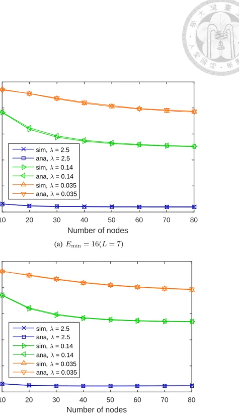
Figure 5.2: The charging time ratio derived from the simulation (sim) and analytical model (ana) under different parameter setting. The parameter E_max = 30, q₀ = 0.3, m₀ = 3 and m = 4

(35)

From Fig 5.2(a), we can see that (i) the device with lower energy harvesting rate may spend more time on replenishing the energy. We also can find out that (ii) the charging time ratio decreases when the number of devices increases. This is because when the number of devices increases, the channel access is harder, and each device will spend more time in backoff states to wait for the next channel access.

But the effect of the number of devices on the charging time ratio is not clear when the energy harvesting rate λ = 2.5. To explain this, we can see Fig 5.3(a). From Fig 5.3(a), we know that for the energy harvesting rate = 2.5, the network can reach the maximum throughput when the number of devices = 10, which means that the channel contention is already saturated. That is why the average charging time will not be changed when we increase the number of devices.

Now we compare Fig 5.2(a) and Fig 5.2(b). In Fig 5.2(b), we change the packet size L from 7 to 2, and from the equation of E_min(Eq. 4.2), the value of E_minis decreased too.

If the number of deivces and the energy harvesting rate are fixed, smaller value of E_min will increase the device operation time and the energy harvesting time simultaneously, so the average charging time ratio will not be changed.

5.2.2 Throughput

Fig. 5.3 compares the average throughput derived from the simulation and our analytical model. In our results, the curves/points labelled “standard” refer to the basic IEEE 802.15.4 protocol in which the devices have no energy constraint (i.e. no energy harvesting state in the model). The analytical model and the simulation result match quite well.

But for the smaller number of devices, the model’s result is slightly different from the sim- ulation. This is because the derivation of β is more accurate for large number of devices.

For further details, please refer to [7].

From the performance evaluation: (i) the throughput of the network with solar energy

(36)

Number of nodes

10 20 30 40 50 60 70 80

Throughput(ratio)

0 0.1 0.2 0.3 0.4 0.5

sim, standard ana, standard sim, 6 = 2.5 ana, 6 = 2.5 sim, 6 = 0.14 ana, 6 = 0.14 sim, 6 = 0.035 ana, 6 = 0.035

(a) Emin= 16(L = 7)

Number of nodes

10 20 30 40 50 60 70 80

Throughput(ratio)

0 0.1 0.2 0.3 0.4 0.5

(b) Emin= 11(L = 2)

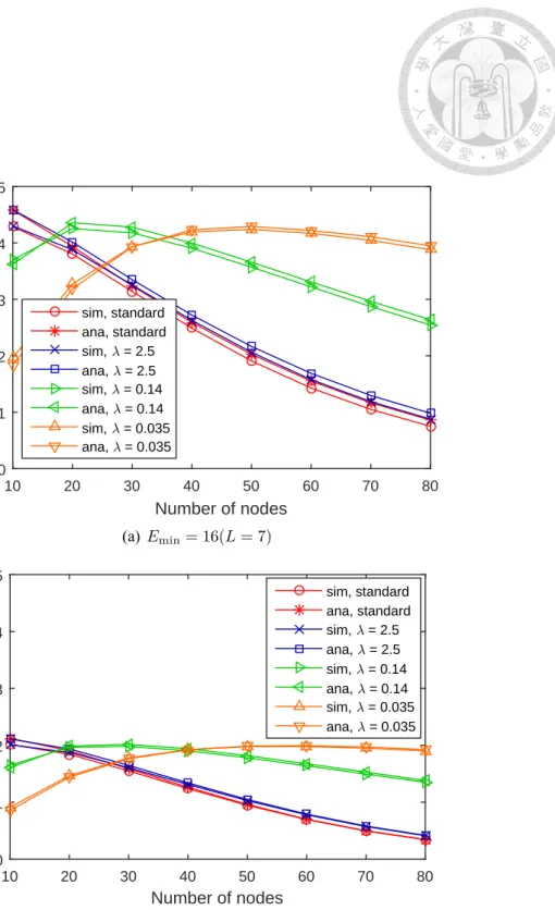
Figure 5.3: The average throughput derived from the simulation (sim) and analytical model (ana) under different parameter setting. The parameter Emax = 30, q0 = 0.3, m₀ = 3 and m = 4

(37)

close to the performance of network without energy constraint. In line with our expecta- tions, there is an upper bound on the throughput. Our evaluation also agrees with results from previous studies that show that energy harvesting directly affects the throughput, but our results go one step further and show that it is range bound (as evidenced by the asymp- totic levelling of throughput). The reasoning behind the better performance is that energy harvesting nodes introduce lesser contention because of their intermittent transmission attempts which essentially reduces the overall attempts on the channel. It is well known that CSMA protocols suffer throughout degradation when large number of nodes compete for access [25], and in this case, the energy harvesting states reduce the number of devices contending for channel access thus improving throughput.

Next, we analyze the throughput of the network with different packet lengths L. By comparing Fig. 5.3(a) and Fig. 5.3(b), we observe that with the same number of nodes and the same energy harvesting rate, the network with longer packet length L has better throughput. When L becomes bigger, the value of E_minincreases, which means that the number of times a device attempts to transmit a packet before the energy harvesting pro- cess starts may decrease. But the simulation result shows that the length of a packet L has more influence than the value of E_minon the network throughput.

5.2.3 Delay

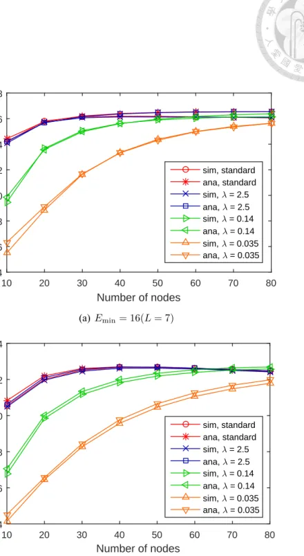
Figure 5.4 plots the average delay versus the number of nodes. The result of the analytical model tracks the simulation result well. We observe that (i) the average delay of the network without the energy constraint is higher than the network with energy harvesting sources, (ii) with the fixed number of nodes, the average delay decreases as the energy harvesting rate decreases, and (iii) with lower energy harvesting rate, the delay increases faster as the number of nodes increases. Those observations fully meet our expectation that the lower energy harvesting rate causes lesser channel contention, and reduces the

(38)

Number of nodes

10 20 30 40 50 60 70 80

Delay(ms)

4 6 8 10 12 14 16 18

(a) Emin= 16(L = 7)

Number of nodes

10 20 30 40 50 60 70 80

Delay(ms)

4 6 8 10 12 14

(b) Emin= 11(L = 2)

Figure 5.4: The average delay derived from the simulation(sim) and analytical model(ana) under different parameter setting. The parameter Emax= 30, q0 = 0.3, m0 = 3 and m = 4

(39)

Emin

14 15 16 17

0 0.2 0.4 0.6 0.8 1

(a) Charging Time Ratio

Emin

14 15 16 17

Throughput(ratio)

0 0.1 0.2 0.3 0.4 0.5

(b) Throughput

Delay(ms)

5 10 15 20 25

(40)

ing rate and the number of nodes, the larger packet lengths yields higher delay, and the delay is exaggerated when the number of nodes increase.

5.2.4 E

_min

and E

_max

In this section, we seek to determine the network performance as a function of pa- rameter E_min and E_max. In Fig. 5.5, we fix the value of packet size L and change the value of m(macMAXCSMABackoffs). With the larger number of m, the number of times that the device performs binary backoff for a packet can be increased. In Fig. 5.5(a) , for λ = 0.035, because the channel usage is low, the device can easily access the channel when NB ( number of backoffs) is small, which means that increasing the value of m has no effect on the charging time when the energy harvesting rate is small. For λ = 0.14, when m is increased, the device may spend more time on the binary backoff, so the average charging time is decreased. For λ = 2.5, since the average charging time with m = 2 is small enough, the decrement of energy charging time is not very obvious when increasing m.

In Fig. 5.5(b), when N = 20, since only the network with λ = 2.5 has optimized the channel usage, the throughput can be increased when we increase the value of m. In Fig. 5.5(c), larger m leads to the smaller probability that a packet is discarded due to the access failure, and more packets can be transmitted by increasing N B, but it will cause the larger average delay.

In Fig. 5.6, we seek to determine the network performance as a function of parameter Emax. We compare the network charging time, throughput and delay with different energy harvesting rate and E_max = 30, 40, 50, and 60. We find that the performance difference is insignificant with increasing E_max. Although larger E_max can let a device work for longer time before entering the energy replenishing process, but the time staying in energy harvesting states is longer too. Hence, we conclude that E_max is not an important factor on the network performance.

Based on the results presented in Figs. 5.2–5.6, we demonstrated that our Markov chain model successfully predicts the behavior of the slotted CSMA/CA protocol of IEEE

(41)

30 35 40 45 50 55 60 Emax

0 0.2 0.4 0.6 0.8 1

(a) Charging Time Ratio

30 35 40 45 50 55 60

Emax 0

0.1 0.2 0.3 0.4 0.5

Throughput(ratio)

(b) Throughput

30 35 40 45 50 55 60

Emax 8

10 12 14 16

Delay(ms)

(c) Delay

(42)

802.15.4 standard with energy harvesting process. Additionally, we reaffirm previous findings [13] that the network performance is indeed different if the energy constraint of each device in considered.