在叢集伺服器上高效能多維奇異值分解及基於閉曲線積分的特徵值分解

(1)

國立臺灣大學理學院應用數學科學研究所碩士論文

Institute of Applied Mathematical Sciences College of Science

National Taiwan University Master Thesis

Efficient Higher-Order Singular Value Decomposition and Contour Integral Based Eigen Decomposition on

CPU/GPU Cluster

蔡宇翔 Yu-Hsiang Tsai

指導教授：王偉仲博士 Advisor: Weichung Wang, Ph.D.

中華民國 107 年 6 月 June, 2018

(2)

(3)

(4)

iv

(5)

誌謝

首先要感謝我的指導教授王偉仲教授，在做研究的途中，老師給予我許多的幫助，例如：協助找到經費讓我能夠出國至國外一流的機構，

去 IBM Thomas J. Watson Research Center 拜訪，去東京大學與那邊的教授和學生互相交流，去 Karlsruhe Institue of Technology 做研究，也讓我能夠去國際會議 SuperComputing 2017 (SC17) 進行報告；另外也帶給我許多機會，像是之前老師與 IBM 的研究人員談完之後，把這個機會介紹給我，而也因此完成了此碩論的第一部份，而當老師出去聽演講或跟別的教授會談之後，常常會試著把專題與別人的應用做連結，讓所做的專題有更廣的應用，像是第二部分的應用部分就是這樣來的。十分感謝老師提供給我如此許多的資源跟機會學習。感謝 Jeewhan Choi 博士、Xing Liu 博士、Takeo Hoshi 教授，在研究上給了我許多的幫助，

讓我在過程中也學習到很多東西。要感謝研究所的同學們，大家時常保持實驗室的氣氛良好，在有遇到困難時也會願意協助，讓許多事情都能夠順順利利完成，在討論時大家也會勇於提出自己的意見與他人交流，保持著很好的學習風氣。要特別感謝林東成和陳彥禎的協助，

常常被我拖著檢查我英文的問題，也常常在溝通之後才發現原來我寫的跟我想表達的常常是兩回事，感謝他們的協助讓我這篇說論能夠順利在時限前完成。最後，謝謝我的家人與朋友的協助，讓我可以無後顧之憂的投入

(6)

vi

(7)

Acknowledgements

First, I am glad to thank my advisor Prof. Weichung Wang. He always gives me a lot of resources and connections. He helps me to find some fund- ing to support me to go aboard to visit the top research place. For example, visit IBM Thomas J. Watson Research Center, discuss projects with the stu- dents and professors of Tokyo University, do some researches in Karlsruhe Institue of Technology, and attend conference SuperComputing 2017 (SC17) to present the student poster. When he attends the speeches and meetings, he always gives me a chance to work with the top researcher or connect my project to different sides. I work with Dr. Jeewhan Choi and Dr. Xing Liu in IBM to finish the first part of my thesis, and also present it on SC17. Prof.

Wang also brings the application of the second part of my thesis. He connects my algorithm and Prof. Takeo Hoshi’s application. Thanks a lot for the mas- sive help of Prof. Wang. Thanks to Dr. Choi, Dr. Liu and Prof. Hoshi. They also give many advisements to me, and I also learn a lot from them. Thanks to classmates of the same laboratory. When I face some problem, they are always enthusiastic to help me. When discussing the paper or something else, they give their comment. I would like to thank Dung-Cheng Lin and Yen- Chen Chen. They help a lot with my English problem. After discussing some paragraph of the thesis, I just discovered the different meaning between what I think and what I write. Due to their help, I can finish the thesis on time.

Finally, I’m glad to thank my family and friends. They allow I can involve the thesis without any problems.

(8)

viii

(9)

摘要

我們改進了 “多維奇異值分解” 及 “基於閉曲線積分的特徵值分解”。

在 “多維奇異值分解” 中，我們使用不同的方式實作兩個演算法，

並提升解決巨量資料的能力。隨著資料越來越多樣，找到方法去快速且有效得壓縮和分析資料中的多角關係對於高效能計算中是非常重要的。我們實做了兩個已經存在的演算法：多維奇異值分解及逐步降維多維奇異值分解將多維矩陣分解，利用 GPU 來加速他們是非常困難的，因為我們幾乎無法把資料一次放進 GPU 的記憶體當中。所以我們利用 QR 和 Gram 來協助我們縮減問題的大小，而我們實作 QR 和 Gram 是將資料分成一部份一部份來解決，這樣不但能讓 GPU 有能力處理，還能利用計算的部分遮蓋掉資料搬移的時間，最後我們相對於原先利用 cuda 函式庫時做的能加速 163.21 倍，在未來希望能夠將這個方法使用在實際問題上。

在 “基於閉曲線積分的特徵值分解” 中，我們藉由基於閉曲線積分的特徵值分解，展示了一個分治法的處理方式去解決區域中有太多的特徵對的問題，並應用它在有機材料模擬。在許多應用上，解特徵值分解扮演了重要的角色，這些矩陣通常都是稀疏的大矩陣，但通常實際上我們只需要一小部分的特徵對，現在有 FEAST 或 CIRR 能夠幫忙解決這類的問題，然而當區域中有許多特徵對時，會變得非常慢，所以必須將問題切成許多小問題。決定分區雖然困難但非常重要，要讓每個小問題都能被輕鬆解決，另外當有些特徵對收料的比較早時，原

(10)

先的方法還是會花時間繼續迭代他們。我們介紹了兩種分區方式：藉由預測特徵對的數量來分解、藉由先備知識來分解。我們提升解決區域中有過多的特徵對問題，且藉由恰當的分區，分治法會比較原先的還快，也利用凍結技巧去讓程式不要花費時間在已經收斂的特徵對上。

之後想設計一個方法能夠讓各個分區解決的時間差不多。

關鍵字：多維陣列、多維奇異值分解、特徵值問題、凍結、閉曲線積分、加速、巨量資料

x

(11)

Abstract

We implement, accelerate, and improve “Higher-Order Singular Value Decomposition” and “Contour Integral based Eigen Decomposition”.

In “Higher-Order Singular Value Decomposition”, we implemented two methods with different strategies and improved the ability to solve the large tensor problem. With the explosion of big data, finding ways of compressing and analyzing large data sets with the multi-way relationship - i.e., tensors - quickly and efficiently have become critical in High-Performance Comput- ing. We implement two existed methods which are Higher-Order Singular Value Decomposition and Sequential Truncated Higher-Order Singular Value Decomposition to achieve Tucker Decomposition. Implementing them with GPU is very difficult because we usually can not store the whole tensor into GPU memory. We use QR method and Gram method to reduce the problem size to make its size allowed by GPU memory. We also implemented QR method and Gram by part-by-part. It can help us to solve the large data problem and use computing to cover data transferring. Finally, We achieve 163.21x speedup over a CUDA library-based solution. In the future, we want to apply it to the real application.

In “Contour Integral based Eigen Decomposition”, we proposed a divide- and-conquer flow to solving the certain eigenpairs in the specific region containing many eigenpairs with eigensolver based on contour integral with the

(12)

locking technique, and use it to solve the generalized eigenvalue problem from the organic material simulation. Solving eigenvalue problems is an essential part of many applications. Those matrices are often large and sparse, but the eigenpairs only are required in the region of interest. Several solvers can solve the eigenpairs in the selected region such as FEAST and CIRR. When there are many eigenpairs in the selected region, the performance is slow, so the partition of the region is needed. Deciding the partition is very difficult but critical such that solving each sub-region should be efficient. When some eigenvector is converged early, the solver still spends time on them. We introduce the two partition method, uniform dividing by the estimated eigenvalue number and dividing by domain acknowledgment. We increase the eigensolver ability to solve the region containing many eigenpairs and get better performance with the proper partition. We also use the locking technique to avoid spending the time on converged eigenpairs. In the future, we would like to design an automatic flow to generate the partition whose sub-region spends almost the same executing time.

Keywords: Tensor, Higher-Order Singular Value Decomposition, General-

ized Eigenvalue Problem, Locking, Contour Integral, Acceralating, Big Data

xii

(13)

List of Figures

3.1 X ≈ G ×^Ni=1A⁽ⁱ⁾ . . . 9

3.2 CUDA SVD is failed when tensor is large . . . 11

3.3 QR-based method . . . 12

3.4 Three QR method overview . . . 12

3.5 Householder QR method can solve large tensor . . . 13

3.6 solve upper triangular matrix by TSQR . . . 16

3.7 Performance of HOSVD with QR methods . . . 17

3.8 STHOSVD vs HOSVD with different rank . . . 17

3.9 Gram method . . . 18

3.10 STHOSVD: Gram method is the fastest algorithm . . . 18

3.11 Gram and QR methods have similar accuracy . . . 19

4.1 the view on different major . . . 22

4.2 the idea of blockQR multigpu . . . 23

4.3 Scalability of multiple GPUs . . . 24

5.1 All Performance . . . 26

7.1 Circle on complex plane . . . 33

9.1 the processing flow . . . 44

11.1 Partition . . . 51

11.2 Overlapped Partition . . . 52

12.1 participation ratio . . . 54

(18)

12.2 the benefit of locking technique . . . 55

12.3 PENTF98736: detail performance . . . 56

12.4 PENTF183600: detail performance . . . 56

12.5 Performance . . . 57

xviii

(19)

List of Tables

1.1 Notation in HOSVD part of this thesis . . . 4

2.1 Names for the Tucker decomposition from [21] . . . 7

6.1 Notation in CI part of this thesis . . . 31

11.1 the computing time of generating list . . . 51

12.1 Performance in one region . . . 55

12.2 PENTF 20400: max-residual . . . 55

12.3 PENTF 98736: max-residual . . . 56

(20)

xx

(21)

Part I

Higher-Order Singular Value

Decomposition

(22)

(23)

Chapter 1 Introduction

Singular Value Decomposition displays a critical role nowadays. We can use it to extract the critical feature and to compress the data. Singular Value Decomposition can find the best rank-n approximation of the matrix. However, we do not just want to analysis the bi-relationship of the data. Thus, we need to explore some ways to find the multi-way relationship.

With the explosion of big data, finding ways of compressing and analyzing large data sets with multi-way relationship - i.e. tensors - quickly and efficiently have become critical in HPC. For example, we want to compress the image with RGB channels. We can use Sin- gular Value Decomposition on each channel before. The image structure is similar in each channel, but applying SVD on each channel is to use same feature to explain it. It leads to the performance is not good. If we use tensor decomposition to compress the image, it also take the relationship of color channel. It can compress the image more efficiently than SVD.

We will introduce Tucker decomposition, which is a kind of tensor decomposition. They are Higher-Order Singular Value Decomposition (HOSVD) and Sequential-Truncated Higher- Order Singular Value Decomposition (STHOSVD). They are easier to implement and do not need much additional knowledge about tensor.

While Higher-Order Singular Value Decomposition (HOSVD) and Sequential-Truncated Higher-Order Singular Value Decomposition (STHOSVD) provide us with the means to attain both extremely high compression ratio and low error rate though low-rank approx-

(24)

imation, optimizing them on accelerators with limited memory is difficult.

We proposed some methods to overcome the two problems of GPU, slow performance in SVD and the memory problem. We use QR methods to make the program not to store whole data in the memory such that GPU can handle much larger tensor than directly implementation. We try different QR method to achieve the better performance in GPU such that the program in GPU have the competitive performance with MKL implementation.

We share our experience and findings on optimizing these algorithms on a node with multiple GPUs, and demonstrate up to 163.21× speedup over a CUDA library-based solution.

The notations used in this part of this thesis are as follows. The regular letters or Latin letters such as a, α, denotes the scalar. The bold lower case letters, such as v, denotes the vectors. The bold uppercase letters, such as A, denotes the matrix. The bold special letters, such asT , denotes the tensor, We show the detail in the Table 1.1

a, α scaler

v, w vector

A, U matrix

T , G tensor

v_i the i-th element of vector

A_ij or A_i,j the (i, j) elemtent of matrix

A_i the i-th column vector of matrix

Ti1i2···iN the (i1, i2,· · · , iN) element of tensor

T(i) the mode-i of tensor

A⁽ⁱ⁾ the i-th matrix A

Table 1.1: Notation in HOSVD part of this thesis

4

(25)

Chapter 2 Preliminary

Tensor is a multi-dimension array. An N-way or Nth-order tensor is an element of N vector space. For example, a vector is a first-order/1-way tensor, a matrix is a second- order/2-way tensor, and the image with RGB color channels is a third-order/3-way tensor.

A third-order tensor whose dimension is I × J × K and elements are real number can be expressT ∈ R^I^×J×K. T (i, j, k) or Tijk is the element (i, j, k) of T . We show some definition and formula of tensors, and [21] shows more detail.

2.1 Tensor Formula

Definition 2.1.1. The norm of a tensorT ∈ R^I¹^×I²^×...×I^N is

∥T ∥ = vu ut∑^I¹

i1=1 I2

∑

i2=1

· · ·

IN

∑

iN=1

Ti²1i2...iN

This is analogous the matrix Frobenius norm.

Definition 2.1.2. Matricization: transforming a tensor into a matrix.

Matricization is known as unfolding or flattening. UseT(n)to express the mode-n matricization of a tensorT ∈ R^I¹^×I²^×...×I^N and the leading dimension ofTnis I_n. We map the

(26)

tensor element (i1, i2, ..., iN) to matrix element (in, j) where

j = 1 +

∑N k=1,k̸=n

(i_k− 1)Jk, with J_k=

k−1

∏

m=1,m̸=n

I_m

The dimension of resulting matrix is In×

∏N i=1,i̸=n

Ii

Definition 2.1.3. Tensor multiplication: the n-mode product.

Tensors can be multiplied together, but it is more complex than the matrix multiplication.

The more detail of tensor multiplication is shown in [1]. We focus the tensor n-mode product, that is, multiplying a tensor by a matrix in mode n.

The n-mode product of a tensorT ∈ R^I¹^×I²^×...×I^N and a matrix A ∈ R^J^×Iⁿ is a tensor whose dimension is I₁× ... × In−1× J × In+1× ... × In. we use operation×nto express n-mode product.

(T ×nU )i1···in−1jin+1···iN =

In

∑

in=1

Ti1i2···iNUjin

The formula can be expressed in terms of flatten tensor.

S = T ×nA ⇐⇒ S(n)= AT(n)

Definition 2.1.4. Vector outer product◦:

T = v⁽¹⁾◦ v⁽²⁾◦ · · · ◦ v^{(N )}

For element,

Ti1i2...iN = v⁽¹⁾_i₁ v⁽²⁾_i₂ · · · v^{(N )}_i_N ∀1 ≤ in≤ IN

We also call the tensorT as a rank-one tensor.

6

(27)

2.2 Tucker Decomposition

The Tucker Decomposition is a form of higher order principal component analysis. It is composed of a core n-way tensor and n matrices.

T ≈ G ×1U⁽¹⁾×2 U⁽²⁾×3· · · ×N U^{(N )} =

I1

∑

i1

· · ·

IN

∑

i_N=1

Gi1...iNU_i⁽¹⁾₁ ◦ · · · ◦ U^{(N )}iN

The tucker decomposition is also denoted byJG; U⁽¹⁾,· · · , U^{(N )}K, and we call G as a core tensor and U⁽ⁿ⁾as factor matrices.

The Tucker decomposition goes by many names mentioned in [21], and they summarized in Table 2.1

Name Proposed by

Three-mode factor analysis (3MFA/Tucker3) Tucker, 1966[35]

Three-mode principal component analysis (3MPCA) Kroonenberg and De Leeuw, 1980[22]

N-mode principal components analysis Kapteyn et al., 1986[17]

Higher-order SVD (HOSVD) De Lathauwer et al., 2000 [2]

N-mode SVD Vasilescu and Terzopoulos, 2002[37]

Table 2.1: Names for the Tucker decomposition from [21]

Remark. Tucker decomposition are not unique.

Let JG; A, B, CK is a Tucker decomposition, and U, V , W are not singular matrices.

Then,

JG; A, B, CK = JG ×1U ×2V ×3W ; AU⁻¹, BV⁻¹, CW⁻¹K

(28)

8

(29)

Chapter 3 Methods and Results

If we wish to find a low-rank approximation to compress or extract significant features from a large data set with the multi-way relationship, Higher-Order Singular Value de- composition allows us to represent the original data with a core tensor,G, and a set of factor matrices along each mode{A⁽ⁱ⁾}^Ni=1.

For example, if we want to store a tensor with dimension 1024× 1024 × 1024, we need 1024³× 8 bytes which are approximate 8 GBs of memory. If we apply HOSVD on this data with the rank of 256, 256, 256, we can reduce its size to a mere≈ 0.13 GB, while retaining most of its properties like Figure 3.1.

Figure 3.1:X ≈ G ×^N_i=1A⁽ⁱ⁾

For a general tensorX with dimensions d1×d2×· · ·×dn, we can calculate a low-rank approximation using the following two algorithms: Algorithm 1: Higher Order Singular Value Decomposition (HOSVD) [2] and Algorithm 2: Sequential Truncated Higher Order Singular Value Decomposition (STHOSVD) [36]

(30)

3.1 Algorithm

We show the algorithms in Algorithm 1 and Algorithm 2.

Algorithm 1 Higher Order Singular Value Decomposition (HOSVD) Require: X , {ri}

Ensure: G, A⁽¹⁾, ..., A^{(N )} for i = 1 to N do

A⁽ⁱ⁾ ← rileading left singular vectors ofX(i) ▷X(i) is mode-i ofX end for

G = X ×1A^(1)⊤×2A^(2)⊤×3...×N A^(n)⊤

returnG, A⁽ⁱ⁾ ▷ tensorG, matrices A⁽¹⁾, ..., A^{(N )}

Algorithm 2 Sequential Truncated Higher Order Singular Value Decomposition (STHOSVD)

Require: X , {ri}

Ensure: G, A⁽¹⁾, ..., A^{(N )} G = X

for i = 1 to N do

A⁽ⁱ⁾ ← rileading left singular vectors ofG(i) ▷G(i)is mode-i ofG G ← G ×iA^(i)⊤

end for

returnG, A⁽ⁱ⁾ ▷ tensorG, matrices A⁽¹⁾, ..., A^{(N )}

The difference between two algorithms is what tensor they use in each iteration. STHOSVD applies SVD on the truncated tensor, so the tensor dimension is reduced in each iteration.

We get the benefit of solving a smaller tensor in each iteration than HOSVD’s. In [36], they show the detail performance and error between two algorithms. We also show the different performance in Figure 3.8

First, we implement these two methods directly in CPU and GPU by MKL and CUDA as our baseline. The implementation by MKL is fast, but we have some troubles in implementation by CUDA.

Remark. Unlike Singular Value Decomposition, the Tucker Decomposition from Algo- rithm 1 and Algorithm 2 is not the best approximation. There are several algorithms to improve the accuracy such as higher-order orthogonal iteration (HOOI) based on HOSVD in [20].

10

(31)

3.2 cuSOLVER SVD

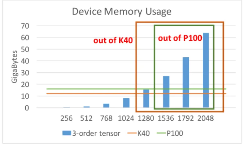
When we implement the HOSVD/STHOSVD by CUDA, one of the critical bottlenecks is calculating the rnleft singular vectors of the matricized tensor. For dense tensors with large mode lengths or large number of modes, these are extremely large matrices that will not fit on the GPU memory. Unfortunately, SVD library provided by NVIDIA’s cuSolver library requires that the entire data set is in memory before it can be factorized, limiting the range of tensors that can be decomposed, and a more scalable solution is required. we show the memory usage of data in Figure 3.2

0 10 20 30 40 50 60 70

256 512 768 1024 1280 1536 1792 2048

GigaBytes

Device Memory Usage

3-order tensor K40 P100 out of K40 out of P100

Figure 3.2: CUDA SVD is failed when tensor is large

Thus, we need to find some methods on GPU to solve the memory problem of GPU.

3.3 QR method

By Definition 2.1.2, we can know the resulting matrix of matricization is usually wide and short when the largest dimension is less than the sqrt of the total number of elements.

Even if the largest dimension is larger than the sqrt of the total number of elements, it only leads to one mode matrix is tall-and-skinny and others still are wide-and-short. Thus, we only focus on how to solve this problem here.

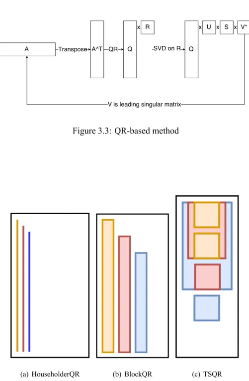
One first solution is to use QR decomposition to reduce the matrix size before finding its singular vectors. We show the flow in Figure 3.3. The matrix is wide-and-short, so we need to transpose it. We do not need to implement transpose if we use row-major to store

(32)

the matrix in CPU. We can do SVD on the upper triangular matrix of QR factorization.

The matrix is much smaller than the original matrix so that GPU can solve its SVD.

Another thing we need to consider, that is, how to solve the QR factorization. If we still use CUDA to solve it entirely in GPU, it still needs whole data in GPU memory, and we face the same problem again. Thus, we need some vector-wise or block-wise QR factorization methods.

Figure 3.3: QR-based method

(a) HouseholderQR (b) BlockQR (c) TSQR

Figure 3.4: Three QR method overview 12

(33)

3.4 Householder QR

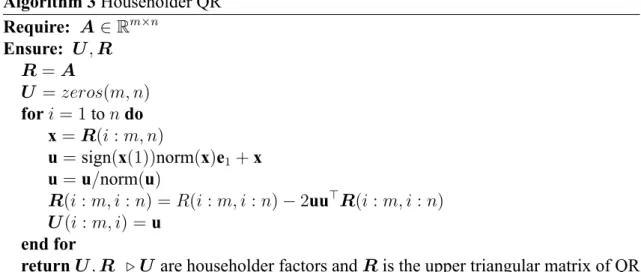
We implemented the commonly used Householder QR method in [4] which allows us to stream the data vector-by-vector Figure 3.4(a), thereby requiring very little device memory. We show the algorithm in Algorithm 3

However, Householder QR has limitation. First, transferring the data vector-by-vector reduces bandwidth utilization. Second, the calculation is composed mostly of BLAS-2 operations, leading to reduced compute utilization

Householder QR is good at calculating HOSVD for large tensors but is slower than cu- Solver SVD due to lower bandwidth and computing utilization in Figure 3.5.

Algorithm 3 Householder QR Require: A∈ R^m^×n

Ensure: U , R R = A

U = zeros(m, n) for i = 1 to n do

x = R(i : m, n)

u = sign(x(1))norm(x)e₁+ x u = u/norm(u)

R(i : m, i : n) = R(i : m, i : n)− 2uu^⊤R(i : m, i : n) U (i : m, i) = u

end for

return U , R ▷ U are householder factors and R is the upper triangular matrix of QR

1.00E+00 1.00E+01 1.00E+02 1.00E+03 1.00E+04 1.00E+05

Time (sec.)

Performance (Householder QR vs CUDA SVD)

HOSVD direct cuda SVD HOSVD Householder QR

cuda SVD is failed because tensor is too large

Better

Figure 3.5: Householder QR method can solve large tensor

(34)

3.5 Modified Block QR

The main idea of Block QR is to compute the block-wise householder factors. We can update the matrix by block-wise factors, and it is more efficient in GPU.

Theorem 3.5.1. A series householder matrix can be a form of (I + W Y^⊤)

Proof. P⁽ⁱ⁾ = I + β_iu⁽ⁱ⁾u^(i)⊤ = I + v⁽ⁱ⁾u^(i)⊤is the matrix from one householder factor.

P is composed of a series P⁽ⁱ⁾

P = P⁽¹⁾P⁽²⁾...P^(r) = (I + v⁽¹⁾u^(1)⊤)(I + v⁽²⁾U^(2)⊤)· · · (I + v^(r)u^(r)⊤)

We show that (I + W Y^⊤)(I + uv^⊤) = (I + ˆW ˆY^⊤), for Y , W ∈ Rⁿ^×kand u, v ∈ Rⁿ^×1

(I + W Y^⊤)(I + vu^⊤) = I + W Y^⊤+ (I + W Y^⊤)(vu^⊤)

= I + [W , (I + W Y^⊤v)][Y , u]^⊤

= I + ˆW ˆY^⊤

where ˆW = [W , (I + W Y^⊤v)]∈ Rⁿ^×(k+1)and ˆY = [Y , u]∈ Rⁿ^×(k+1)

We do it recursively on the series of P⁽ⁱ⁾, so we can get P = (I + W Y ) for some W , Y

In algorithm 4 line 13, there are two Mat-vec operations. However, the Blas-2 operations are slow in GPU, so we modify a little part of these codes to make it more powerful.

In algorithm 5, there are only one Mat-Mat operation (line 10) out of for-loop and one Mat-Vec operation (line 14) in for-loop.

We replace r level-2 operation with one level 3 operation. It is more suitable in GPU than the original one.

By using extra device memory, modified Block QR (Figure 3.4(b)) combines several Householder factors into two matrices to increase the memory throughput. Modified

14

(35)

Algorithm 4 Block QR Require: A, r

Ensure: Q, R

1: Q = I

2: for k=1:n/r, s=(k-1)r+1 do

3: for j=1:r do

4: u = s + j− 1

5: [V , β] = house(A(u : m, u))

6: A(u : m, u : s + r− 1) = (I + βvv^⊤)A(u : m, u : s + r− 1)

7: V (:, j) = [zeros(j− 1, 1); v], b(j) = β

8: end for

9: Y = V (1 : end, 1)

10: W = b(1)V (1 : end, 1)

11: for j=2:r do

12: v = V (:, j)

13: z = (I + W Y^⊤)v

14: W = [W , b(j)z], Y = [Y , v]

15: end for

16: A(s : m, s + r : n) = (I + Y W^⊤)A(s : m, s + r : n)

17: Q(1 : m, s : m) = Q(1 : m, s : m)(I + W Y^⊤)

18: end for

Algorithm 5 Modified Block QR Require: A, R

Ensure: Q, R

1: Q = I

2: for k=1:n/r, s=(k-1)r+1 do

3: for j=1:r do

4: u = s + j− 1

5: [v, β] = house(A(u : m, u))

6: A(u : m, u : s + r− 1) = (I + βvv^⊤)A(u : m, u : s + r− 1)

7: V (:, j) = [zeros(j− 1, 1); v], b(j) = β

8: end for

9: Y = V

10: C = V^⊤V

11: W = b(1)V (1 : end, 1)

12: for j=2:r do

13: v = V (:, j)

14: z = v + W ∗ C(1 : j − 1, j)

15: W = [W , b(j)z], Y = [Y , v]

16: end for

17: A(s : m, s + r : n) = (I + Y W^⊤)A(s : m, s + r : n)

18: Q(1 : m, s : m) = Q(1 : m, s : m)(I + W Y^⊤)

19: end for

(36)

Block QR has the more blas-3 operation than Householder QR. Not surprisingly, Modi- fied Block QR is faster than Householder QR. Also, we only need some column blocks of the matrix in GPU memory, so we can also solve larger data. However, when the matrix is tall, the corresponding block used in modified Block QR is too skinny to utilize the compute units fully and reduces the overall performance (much like the Household QR case).

3.6 Tall Skinny QR

R

Figure 3.6: solve upper triangular matrix by TSQR

We can only compute the upper triangular matrix of QR factorization in Figure 3.3, so we show how to solve it by tall skinny QR in Figure 3.6. How to solve Q matrix by TSQR and more details are shown in [3].

TSQR is more suitable for this problem than Block QR because it splits the rows to avoid the above situation. It divides the matrix into several square blocks in a column.

To solve the QR problem, we solve the QR factorization for two adjacent blocks indepen- dently and combine them. Inductively, it forms the whole process.

We explored using Tall Skinny QR - TSQR (Figure 3.4(c)) to overcome the throughput is- sues. Moreover, we do not need to solve Q of QR by TSQR, so we reduce many operations

16

(37)

to achieve better performance. Modified Block QR and TSQR significantly improve the performance of the HOSVD algorithm. The performance of them are shown in Figure 3.7

1.00E+00 1.00E+01 1.00E+02 1.00E+03 1.00E+04 1.00E+05

Time (sec.)

Performance

HOSVD direct cuda SVD HOSVD Householder QR HOSVD TSQR

HOSVD BlockQR Rank of problem has small

influence on performance

Better

Figure 3.7: Performance of HOSVD with QR methods

Modified Block QR and TSQR improve performance over the Householder QR and cuSolver SVD methods. However, HOSVD’s performance is independent of the rank.

Even if we want just a small rank approximation of the tensor, we need to spend similar time computing it like computing full rank approximation.

Therefore, we introduce the STHOSVD method that can further improve the performance, and reduce the overall work when the rank is smaller by calculating the Tensor-Times Matrix (TTM) step within the inner loop.

0 0.5 1 1.5 2 2.5

Speedup

Low Rank Effort

HOSVD BlockQR STHOSVD BlockQR compared with 1024->1024 comparedwith 2048->1024

Better

Figure 3.8: STHOSVD vs HOSVD with different rank

(38)

3.7 Gram Method

Besides QR methods we also use Gram method followed by eigenvalue decomposition to solve the problem (Figure 3.9(a)). In this process, we multiply the matricized tensor by its transpose and regard the initial SVD problem as an eigenvalue problem of Gram matrix with smaller problem size (Figure 3.9(b)).

(a) Gram flow (b) Gram

Figure 3.9: Gram method

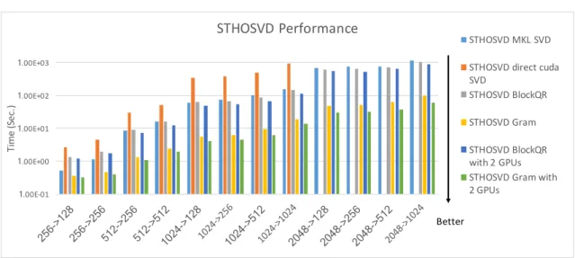
The block multiplications used in Gram method are independent, so we can interleave the matrix transfer with computation to increase efficiency, and then combine it with the STHOSVD method to increase performance. The Performance of STHOSVD is shown in Figure 3.10

1.00E-01 1.00E+00 1.00E+01 1.00E+02 1.00E+03

Time (Sec.)

STHOSVD Performance

STHOSVD MKL SVD STHOSVD direct cuda SVD

STHOSVD BlockQR STHOSVD Gram STHOSVD BlockQR with 2 GPUs STHOSVD Gram with 2 GPUs

Better

Figure 3.10: STHOSVD: Gram method is the fastest algorithm 18

(39)

3.8 Error

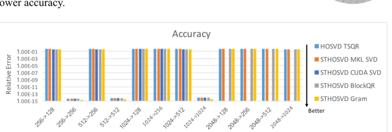
We generate the dense tensor with random numbers whose condition number is small, so the accuracy of QR method and Gram method are competitive in Figure 3.11. The random generating tensor is not main structure inside itself, so the non-full rank approximation is lower accuracy.

1.00E-15 1.00E-13 1.00E-11 1.00E-09 1.00E-07 1.00E-05 1.00E-03 1.00E-01

Relative Error

Accuracy

HOSVD TSQR STHOSVD MKL SVD STHOSVD CUDA SVD STHOSVD BlockQR STHOSVD Gram Better

Figure 3.11: Gram and QR methods have similar accuracy

(40)

20

(41)

Chapter 4 Implementation

4.1 Transpose

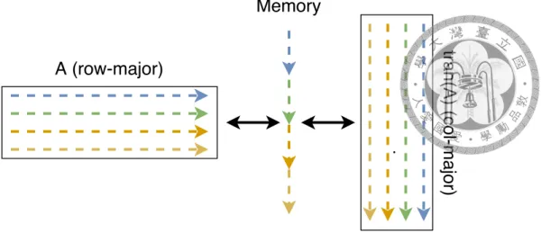
For the QR methods, the transpose of the matrix we need to consider. However, when we store the matrix row-major in CPU, we can do the transpose implicitly. In the memory, the data is stored as sequential, that is, A is stored as A₁₁A₁₂A₁₃· · · A1MA₂₁· · · AN M

(row-major) in CPU memory. When we move the data to GPU sequential, the ordering of elements is still the same. The function provided by NVIDIA is for column-major so that the function will see the transpose of A

In GPU view, such as Figure 4.1,







A₁₁ A₂₁ · · · AM 1

A₁₂ A₂₂ · · · AM 2

... . .. ... ... A_1N A_2N · · · AM N







=







A^⊤₁₁ A^⊤₁₂ · · · A^⊤1M

A^⊤₂₁ A^⊤₂₂ · · · A^⊤2M

... . .. ... ... A^⊤_{N 1} A^⊤_{N 2} · · · A^⊤_{N M}







= A^⊤

(42)

A (row-major)

Memory

tran(A) (col-major)

Figure 4.1: the view on different major

Similarly, we can get back the V^⊤back to GPU without transpose.

Remark. In cuSolver 8, 9.0, 9.1, 9.2, the routine cusolverDn<t>gesvd returns V^⊤ not V for real number.

4.2 CUDA Stream

We use CUDA stream on GPU to schedule the works. The different streams are ’almost’

independent, so the GPU can do several small tasks at the same time if they can. The stream thought is also between different GPU. If there is no constraint, the streams in different GPUs are really independent. In Section 4.3, we use two GPU to do the updating step at the same time. For BlockQR, Housholder QR Blas-2 operation, we also use several streams to do it.

Remark. The streams mentioned here are not the default stream.

Whether the function can be run simultaneously in several streams of the same GPU de- pends on the number of SM function using, or data movement, etc.

22

•

(43)

4.3 Multiple GPUs

1 Build Householder Block

1 Update Matrix

Dependence: 'Update' must be after 'Build' with same number

1 1

1

1 1

GPU 0 2 GPU 1

2 2

Figure 4.2: the idea of blockQR multigpu

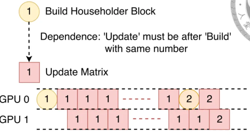
Householder QR (Figure 3.4(a)) and Block QR (Figure 3.4(b)):

We implement Householder QR and Block QR block-wise. The information also updates block-wise. These methods update simultaneously on multiple GPUs. We make one GPU update fewer blocks than the other GPUs and solve QR factorization of the next block when other GPUs still update the remaining blocks. We show the idea in Figure 4.2. With this schedule, the next round updating step does not need to wait for the QR factorization.

• TSQR (Figure 3.4(c)):

We split a matrix into several tall and skinny blocks by the number of GPUs. We use TSQR to solve each block, so it is an independent process. And then we combine the results together in a single matrix and apply TSQR method on this matrix.

• Gram method (Figure 3.9(b)):

We split the matrix into several small blocks. For each block, we only need to calculate the product of its transpose and itself. The operations in each block are independent so that we can assign those works to multiple GPUs equally.

(44)

0 0.5 1 1.5 2 2.5

Scalability

Multiple GPUs Effort (2 GPUs vs 1 GPU)

HOSVD TSQR STHOSVD BlockQR STHOSVD Gram Better

Figure 4.3: Scalability of multiple GPUs

24

(45)

Chapter 5 Conclusion

We study and optimize four methods - Householder QR, Modified Block QR, TSQR, and Gram method - to solve the SVD step in HOSVD and STHOSVD. QR methods implemented by the vector-wise or the block-wise algorithm can solve the GPU memory problems. Among these QR methods, TSQR is the fastest one. TSQR can ignore the computing Q step, and it uses row block which is more suitable for our problems.

We also use another algorithm, Gram method. Among them, Gram method is the fastest algorithm and the Simplest to implement, and provides comparable accuracy in less time when the condition number of the tensor is small.

Although QR methods are slower than Gram method, in the case that the condition number of the original tensor is large, it may provide higher accuracy.

For the overall performance, we show it in Figure 5.1 or figure in https://goo.gl/QsovD1.

(46)

1.00E-01 1.00E+00 1.00E+01 1.00E+02 1.00E+03 1.00E+04 1.00E+05 256->128256->256512->256512->5121024->1281024->2561024->5121024->10242048->1282048->2562048->5122048->1024

Time (Sec.)

All Performance

HOSVD direct cuda SVDHOSVD Householder QRHOSVD MKL SVDHOSVD BlockQRHOSVD TSQRHOSVD TSQR with 2 GPUs

STHOSVD direct cuda SVDSTHOSVD MKL SVDSTHOSVD BlockQRSTHOSVD BlockQR with 2 GPUsSTHOSVD GramSTHOSVD Gram with 2 GPUs Better

Figure5.1:AllPerformance

26

(47)

Part II

Contour Integral based Eigenvalue

Decomposition

(48)

(49)

Chapter 6 Introduction

Solving eigenvalue problems is an important part of many applications. Those matrices are often large and sparse but the eigenpairs only are required in the region of interest.

Several solvers can solve the eigenpairs in selected regions such as FEAST and CIRR.

FEAST is a density-matrix-based algorithm proposed by Polizzi [27] [26], [19]. CIRR is the Raleigh-Ritz-type approach of the contour integral eigensolver proposed by Ikegami and Sakurai [29], [12], [13], [16]. These eigensolvers are extended to solve non-Hermitian eigenvalue problems. The numerical analysis are shown in [16] and [26]

These eigensolvers require inputs of columns of the initial subspace. If the initial subspace is too small, it can not solve the eigenpairs in the region of interest. There are some algorithms for estimating the number of eigenpairs in certain region in [5], [6], and [24]. We use the estimated number of the eigenpairs as the number of columns of initial subspace with the scale (we use 1.5 as the scale). That is, #{cols of subspace} =

⌈scale(1.5) × #{estimation}⌉. The estimated number is only used to build the initial sub- space. Moreover, FEAST also estimates the number of the eigenpairs in second loop [26], and it uses its estimated result in stopping criterion.

Partition of the region is a crucial part of solving generalized eigenvalue problems by the eigensolver based on contour integral. The eigensolver based on contour integral is a powerful tool to solve the whole eigenpairs in a given region for generalized eigen-

(50)

value problem. In some applications, there are many eigenpairs in the region. It increases the difficulty of the problem. We can separate the original region into several sub-regions whose union is the original one. However, it will solve some eigenpairs repeatedly in their intersections. Thus, the deflating technique is needed to avoid these problems. Based on deflating technique, we introduced a divide-and-conquer method on the eigensolver based on contour integral.

The deflating technique can remove those repeated eigenpairs we have solved. The matrices are sparse, so we can explicitly form the deflated matrices. It will turn the matrices into dense matrices. We can use Woodbury Identity Theorem to solve the linear systems without building matrices explicitly, but it will increase the number of linear systems [7]. Locking technique [31], [28] is known as an implicit deflating technique. It may lead the convergence problem [31], but it can decrease the number of linear systems by removing solved vector out of the searching base. In [39], they show how to apply locking technique in FEAST for solving Hermitian standard eigenvalue problems.

This paper discusses the dividing-and-conquer method with locking technique based on FEAST for solving Hermitian generalized eigenvalue problems and shows how to apply the locking technique to generalized eigenvalue problems with some condition and discuss the performance between different kinds of partition, such as auto-partition and pre-knowledge partition. We choose the PENTF cases from [9] as our testing data. We show the benefits of locking, and the fact that partition is helpful when solving much larger problems and sometimes accelerate the solving process.

The notations used in this part of this thesis are as follows. The regular letters or Latin letters such as a, α, denotes the scalar. The bold lower case letters, such as v, denotes the vectors. The bold uppercase letters, such as A, denotes the matrix. We show the detail in the Table 6.1

30

(51)

a, α scaler

v vector

A matrix

vi the i-th element of vector

A_ij or A_i,j the (i, j) elemtent of matrix

A_i the i-th column vector of matrix

A⁽ⁱ⁾ the i-th matrix A

A[k] specified the column of matrix.

Table 6.1: Notation in CI part of this thesis

(52)

32

(53)

Chapter 7 Preliminary

7.1 Eigensolver based on Contour Integral

We consider a circle in the complex plane, and we call the boundary Γ and the interior Ω such as Figure 7.1. Eigensolver based on Contour Integral computes some equations on the quadrature points to get the basis of the eigenpairs in the Ω. After building the basis, we project the original matrix pairs on this basis to form a smaller generalized eigenvalue problem than the original one. Then we solve its eigenpairs, and we can reconstruct the eigenpairs in the interior Ω of the original matrix pair A, B. We will introduce some algorithm in later.

Figure 7.1: Circle on complex plane

(54)

7.2 Quadrature rules

We need to calculate the equations of the contour integral numerically. Thus, we introduce some quadrature rules show how to build up x, w of P quadratic points for k = 1· · · P . It is gotten from [39]

• midpoint rule:









x_k = 2k− 1 2P w_k = 1

P

• Gauss-Chebyshev rule for the first kind:









x_k = 1

2(1 + cos((2k− 1)π

2P ))

w_k = 2π

P sin((2k− 1)π

2P )

• Gauss-Chebyshev rule for the second kind:









xk = 1

2(1 + cos( kπ P + 1)) w_k = 2π

P sin( kπ P + 1)

• Gauss-Legendre rule:









x_k = t_k+ 1 2

w_k = 1

(1− t²k)(L^′_P(t_k))²

where t_kis the k-th root of the pth Legendre polynomial L_P(x)

Among these quadratic rule, the Gauss-Legendre rule (Section 7.2) is popular. MKL FEAST and our implementation use this rule.

Remark. For using Section 7.2, we need to compute the point z on the circle boundary Γ 34

(55)

θ_k=−π

2(x_k− 1) zk = c + re^iθⁱ

wk ← −w_k 2

By the way, we implement the complex Hermitian version on the eigensolver. The quadratic point of the lower part is conjugate with those point of the upper part, and weight is not changed.

(56)

36

(57)

Chapter 8 Theorem

8.1 Deflation

The original generalized eigenvalue problem is given by

Ax = λBx

If all eigenvectors are B-orthonormal, we can use the following deflation technique.

Let a set{y}j is B-orthonormal, i.e. ,

y^∗_iBy_j =









0 i̸= j 1 i = j

Collect those eigenvectors we have solved in S.

y is an eigenvector. Ay = λBy

Consider ˜A = A + σB(∑

v∈S

vv^∗)B^∗. If y∈ S, then ˜Ay = Ay + σB(∑

y∈S

vv^∗)B^∗y = λBy + σBy = (λ + σ)By.

If Y /∈ S, then ˜Ay = Ay + σB(∑

v∈S

vv^∗)B^∗y = λBy + 0 = λBy.

By applying such deflation technique, the eigenvectors belonging to S can be removed from S

(58)

8.2 Theorem

The method can be applied to these problems which satisfy the following conditions.

Condition 8.2.1.

∀{λ, x} eigenpairs, Ax = λBx ⇐⇒ A^∗x = λ^∗B^∗x (8.1)

∀x, y, ⟨x, By⟩ = ⟨Bx, y⟩ (8.2)

Theorem 8.2.2. If Ax = λBx and A^∗x = λ^∗B^∗x, then the eigenvectors with distinct eigenvalues are B-orthogonal.

Proof. Write Ax = λBx and Ay = µBy, which λ̸= µ

⟨y, Ax⟩ = y^∗λBx = λy^∗Bx

⟨y, Ax⟩ = ⟨A^∗y, x⟩

⟨A^∗y, x⟩ = ⟨µ^∗B^∗y, x⟩ = y^∗Bµx = µy^∗Bx

0 =⟨y, Ax⟩ − ⟨A^∗y, x⟩ = (λ − µ)y^∗Bx λ̸= µ, so y^∗Bx = 0. i.e. they are B-orthogonal.

Note that, in this argument, condition(2) are not required.

Theorem 8.2.3. Ax = λBx, A^∗x = λ^∗B^∗x, and⟨x, By⟩ = ⟨Bx, y⟩. The eigenvec- tors with identical eigenvalues can be reformulated as B-orthogonal eigenvectors with the same eigenvalues.

Proof. By collecting independent eigenvectors with identical eigenvalues, we can recon- struct an orthonormal eigenvector with the same eigenvalue via linear combination.

y =

∑r i=1

a_ix⁽ⁱ⁾

Ay = A

∑r i=1

a_ix⁽ⁱ⁾ =

∑r i=1

a_iAx⁽ⁱ⁾ =

∑r i=1

a_iλBx⁽ⁱ⁾ = λB

∑r i=1

a_ix⁽ⁱ⁾ = λBy

38

(59)

Thus, the eigenvalue of a linear combination of eigenvectors remains the same

One can re-scale them to make it B-orthonormal. For example, x and y are eigenvectors with same eigenvalue. Assume⟨x, By⟩ = k is not B-orthonormal. we denote ˆy = y−kx.

Then,

⟨x, Bˆy⟩ = ⟨x, B(y − kx)⟩ = ⟨x, By⟩ − ⟨x, kx⟩ = k − k = 0

⟨ˆy, Bx⟩ = ⟨(y − kx), Bx⟩ = ⟨y, Bx⟩ − ⟨kx, x⟩ = ⟨ atBx, y⟩ − k = k − k = 0

Theorem 8.2.4. Ax = λBx, A^∗x = λ^∗B^∗x and⟨x, By⟩ = ⟨Bx, y⟩. One can construct a collection of B-orthogonal eigenvectors.

Proof. Under the Condition 8.2.1, this is the direct conclusion from previous theorems.

Theorem 8.2.5. B is and Hermitian matrix and B = LL^∗. If A = LU DU^∗L^∗, where U is a unitary matrix and D is a diagnol matrix, this matrix pair (A, (B)) satisfied our conditions. That is, L⁻¹AL^∗−1is a normal matrix.

Proof.

Ax = λBx

LM DM^∗L^∗x = λLL^∗x

(LM )D(M^∗L^∗)x = λ(LM )(M^∗L^∗)x Disadiagnalmatrix, soλarethediagnalvalue

A^∗x = µB^∗x LM D^∗M^∗L^∗x = µLL^∗x

D^∗isadiagnalmatrix, soµarethediagnalvalue

Thus, µ is conjugate of λ

8.3 Cases

1. A is a symmetric matrix, and B is a symmetric positive definite matrix.

(60)

2. A is a Hermitian matrix, and B is a Hermitian positive definite matrix.

3. B is a Hermitian positive definite matrix, and L⁻¹AL^∗−1is a normal matrix

These cases satisfy our condition. The eigenvalues can be complex in some cases.

40

(61)

Chapter 9 Algorithm

Denote

ρ(A, B, z, w)Q =

∑N i=1

w_i(z_iB− A)⁻¹Bq ,where z and w are quadratic points shown in Section 7.2

9.1 Estimation

We choose the estimation method shown in [6] becasue its linear systems are similar with those of FEAST(Algorithm 7). Thus, we can reuse the implementation of solving the linear systems.

Algorithm 6 estimate the number of eigenvalue in the circle in [6]

Require: A, B, z, w

Ensure: the estimated number of eigenvalue in the circle

1: Initial the random matrix: Q

2: Approximate subspace projection: Y ← ρ(A, B, z, w)Q

3: Calculate the trace: 1 PQ^⊤Y

9.2 FEAST

The Algorithm 7 is declared in [26]. We use this algorithm as our main eigensolver.

在叢集伺服器上高效能多維奇異值分解及基於閉曲線積分的特徵值分解

Institute of Applied Mathematical Sciences College of Science

National Taiwan University Master Thesis

誌謝

Acknowledgements

摘要

Abstract

Contents

I Higher-Order Singular Value Decomposition 1

II Contour Integral based Eigenvalue Decomposition 27

Bibliography 61

List of Figures

List of Tables

Part I

Higher-Order Singular Value

Decomposition

Chapter 1 Introduction

Chapter 2 Preliminary

2.1 Tensor Formula

2.2 Tucker Decomposition

Chapter 3

Methods and Results

3.1 Algorithm

3.2 cuSOLVER SVD

3.3 QR method

3.4 Householder QR

3.5 Modified Block QR

3.6 Tall Skinny QR

R

R

R

R

R

R

R

Low Rank Effort

3.7 Gram Method

3.8 Error

Chapter 4

Implementation

4.1 Transpose

4.2 CUDA Stream

4.3 Multiple GPUs

Chapter 5 Conclusion

Part II

Contour Integral based Eigenvalue

Decomposition

Chapter 6 Introduction

Chapter 7 Preliminary

7.1 Eigensolver based on Contour Integral

7.2 Quadrature rules

Chapter 8 Theorem

8.1 Deflation

8.2 Theorem

8.3 Cases

Chapter 9 Algorithm

9.1 Estimation

9.2 FEAST