行政院國家科學委員會專題研究計畫 成果報告
兩帶電液滴間之動態交互作用探討:理論與實驗
計畫類別: 個別型計畫
計畫編號: NSC93-2212-E-011-037-
執行期間: 93 年 09 月 01 日至 94 年 07 月 31 日 執行單位: 國立臺灣科技大學機械工程系
計畫主持人: 蘇裕軒
計畫參與人員: 賴彥豪 張立翰 黃百源
報告類型: 精簡報告
處理方式: 本計畫可公開查詢
中 華 民 國 94 年 8 月 1 日
行政院國家科學委員會專題研究計劃成果報告 兩帶電液滴間之動態交互作用探討
計劃編號 : NSC 93-2212-E-011-037 執行期限 : 93年09月01日至94年07月31日 主持人 : 蘇裕軒 (國立台灣科技大學機械工程研究所)
參與人員 : 賴彥豪、 張立翰、 黃百源 (國立台灣科技大學機械工程研究所)
中文摘要
因兩帶電液滴間之動態交互作用在科學與工程等諸方面之應 用, 一直以來其研究深受研究人員重視。 本研究利用邊界積分 方程, 求解三個控制兩個軸對稱、 非黏性帶電液滴運動之拉普 拉斯方程式, 並以四階之 Rung-Kutta 數值法, 積分該系統 之動態方程, 來模擬帶電液滴之互制行為。 研究發現, 靜電交 互作用對於帶電液滴之運動, 僅有局部影響, 且其影響只在液 滴非常接近時才有顯著作用。 綜此, 以 Legendre modes 為 基礎之整體分析並不適用於帶電液滴間之靜電交互作用行為 探討。 故而, 本研究將藉由一些有趣之案例, 來探討各種方式 之靜電互制行為。
Abstract
With numerous applications prevailing in science and engineering, the dynamics of charged droplets held together by surface tension and coupled together via electrostatics is of great interest to many researchers.
In this work, boundary integral method is used to solve the three Laplace equations governing the dy- namics of the two axisymmetric, inviscid charged droplets. Time integration of the associated dynami- cal system is achieved using the fourth order Runge- Kutta method. The present results suggest that the electrostatic interaction has only localized effect on the motions of the two coupled droplets. Global analysis based upon Legendre modes may not be a meaningful approach in the current study. Conse- quently, some interesting aspects of the dynamics of two electrostatically coupled charged droplets are il- lustrated via various examples.
Keywords:
Charged droplets; Electrostatics;Coulomb attraction; Boundary-integral method;
Legendre modes.
1 Introduction
Since charged droplets are usually self-dispersive, they play significant roles in industrial applications such as electrospray atomization [1], [2], [3], [4], fuel injection, ink-jet printing, and formation of clouds.
Obviously, the dynamic interactions between two charged droplets are of essential importance to these applications and, if controlled, can be applied to en- hance separation or coalescence of small droplets. De- spite its extensive industrial applications, a funda- mental understanding of the underlying physics of the dynamic interactions between charged droplets is still lacking.
Droplets can be charged via a number of means in- cluding direct contact, induction, conduction, charge injection using electron gun, and atmospheric charg- ing. The maximum charge that a single droplet can sustain is called the Rayleigh’s limiting charge Q
(2) R
, which can be expressed as follows:Q (2) R
= πp(8²
0 σd 3
),where σ and d are the surface tension and diameter of the droplet, respectively; ²
0
is the electrical per- mittivity of vacuum. The droplet becomes unstable when charged beyond Q(2) R
and jets may form at the tips of the charged droplet [5], [6], [7]. The liquid jets will further break up into smaller droplets to achieve the surface charge redistribution.Various aspects of the dynamics of a single charged droplet have been extensively studied. The
study of the equilibrium shape and linear stabil- ity of a single charged droplet dated back to Lord Rayleigh’s investigation [8]. Bifurcation near the Rayleigh’s limiting charge has been extensively stud- ied [9], [10], [11], and [12].
Disintegration/breakup of droplets associated with surface instability resulted from the modal in- teraction between linearly independent shape oscilla- tions is also possible [14]. The nonlinear shape os- cillations of a single charged droplet near breakup have been studied extensively with asymptotic ex- pansion method [9], [10], [11], [12], [13]. The shape oscillations of two charged droplets are further com- plicated by the electrostatic interaction between the two droplets and the asymptotic method becomes ex- tremely tedious and difficult for this case. Hence lit- erature on the investigation of interactions between two charged droplets is extremely scarce.
The purpose of this study is to investigate the dy- namic interactions between two charged droplets un- der various combinations of physical parameters such as sizes, velocities, charges, and surface tension of the droplets. We are also interested in the possible en- ergy transfer from higher modes (shape oscillations) to fundamental mode (translational motion) due to the electrostatic effects associated with the nonlinear vibrations.
Experimental observation revealed that coales- cence of droplets is also possible between a charged droplet and an uncharged (but polarized) droplet due to Coulomb attraction [15]. Obviously this can be used to explain the formation of clouds and precipita- tion. More intriguingly, we would like to explore how the shape oscillations of the charged droplet would change the Coulomb attraction.
2 Governing Equations
In this work, the liquid droplets are assumed to be inviscid, incompressible, and electrically conduc-
tive. No mass exchange across the interfaces and
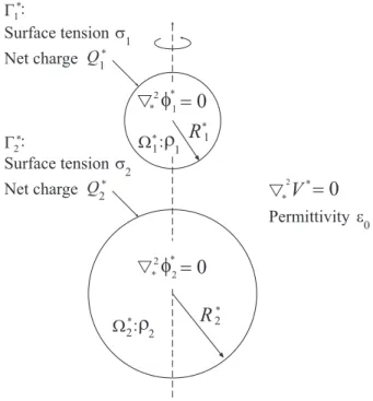
thermal conduction within the droplets are consid- ered in the model. The problem to be considered is shown schematically in Figure 1. The two incom- pressible liquid droplets have densities ρ
1 , ρ 2
, uniform surface tensions σ1 , σ 2
, equivalent radii R1 ∗ , R 2 ∗
, and net charges Q∗ 1 , Q ∗ 2
residing on their surfaces, respec- tively. Let Ω∗ 1
(t∗
), Ω∗ 2
(t∗
) be the interior space oc- cupied by the two droplets and Γ∗ 1
(t∗
), Γ∗ 2
(t∗
) be the surfaces of the two droplets at time t∗
, respectively.For the purpose of scaling that will be introduced later, all the physical variables are introduced with an asterisk as superscript. The operator ∇
∗
is also introduced for the same purpose.Let U
∗ 1 , U ∗ 2
be the velocity fields within droplets 1 and 2, respectively. If the flow inside each droplet is assumed to be a potential flow with velocity potentialφ ∗ i
(i = 1, 2), thenU ∗ i
= ∇∗ φ ∗ i
(i = 1, 2). (1) From the mass conservation of incompressible fluid we know the hydrodynamic fields are governed by∇ 2 ∗ φ ∗ i
= 0,∀x ∗ ∈ Ω ∗ i .
(2) The governing equation, Eq.(2), applies to both steady and unsteady flow. Yet no dependence of time appears explicitly in this equation. This implies that as a result of incompressibility, the irrotational flow can be determined by the instantaneous boundary conditions. In other words, any change in the bound- ary conditions propagates through out the whole do- main immediately. Consequently, the velocity poten- tial can be fully determined from the status quo of boundary data without using any information from the dynamic boundary condition1
.The Navier-Stokes equation for an inviscid fluid in the absence of body forces other than gravitational force can be expressed as
ρ i
·
∂U ∗ i
∂t ∗
+ (U∗ i · ∇ ∗
) U∗ i
¸
= −∇
∗ P i ∗ − ρ i gk in Ω ∗ i ,
(3) where Pi ∗
is the pressure field within i-th droplet, andg the gravitational constant.
1
A wave equation has to be solved, if the compressibility were accounted for. The second order time derivative term in the
wave equation relies on information coming from the dynamic boundary condition, thus the wave equation can not be solved
independently. All three equations are coupled and must be solved simultaneously.
Substituting U
∗ i
= ∇∗ φ ∗ i
into Eq.(3) and integrat- ing the resulting equation with respect to the spatial variables yields the unsteady Bernoulli’s equationρ i ∂φ ∗ i
∂t ∗
+12
ρ i ∇ ∗ φ ∗ i ·∇ ∗ φ ∗ i
+Pi ∗
+ρi gz ∗
= h∗
(t∗
) in Ω∗ i ,
(4) where h∗
(t∗
) is an arbitrary function of time only2
.Let V
∗
be the electric potential of the free space, then the governing equation for the electric field can be written as follows:∇ 2 ∗ V ∗
= 0,∀x ∗ ∈ R 3 \(Ω ∗ 1 ∪ Ω ∗ 2
). (5) Since the two liquid droplets are conductive, V∗
is constant on the two droplet surfaces, respectively. i.e.V ∗
= Vi ∗
on Γ∗ i .
(i = 1, 2) (6) From the Gauss’s theorem in electrostatics, we knowIΓ
∗i(n
i · ∇ ∗ V ∗
) dA = −Q ∗ i
² 0 ,
(i = 1, 2) (7) where ni
is the normal vector on the droplet surface Γ∗ i
.Since there is no external electric field applied at infinity, we can set
V ∗ → 0
as x∗ → ∞.
(8) The dynamical boundary conditions, governed by the Laplace-Young equation including the electric stress due to the surface charge, can be expressed asP i ∗ −P o ∗
= σi ∇ ∗ ·n i
+ µ−² 0 ∂V ∗
∂n i
¶ µ1 2
∂V ∗
∂n i
on Γ
∗ i ,
(9) where Po ∗
is the pressure of the surrounding medium immediately outside the interface and ni
the outward unit normal on the interface Γ∗ i
. The term ∇∗ ·n i
rep- resents the total curvature of a generic point on the interface. Note that the electric field on the inter- face is1 2 ∂V ∂n
∗i due to the charge discontinuity across
the interface [16]. Furthermore, the sign of the term associated with electric charge is opposite to that of the term associated with surface tension. This corre- sponds to the fact that surface tension smooths out the curvature on the drop surface while the electric charge moves to location of high curvature and be- comes a destabilizing force.
Combining Eq. (4) and (9) gives
ρ i ∂φ ∗ i
∂t ∗
+12
ρ i ∇ ∗ φ ∗ i · ∇ ∗ φ ∗ i
+ Po ∗
+ σi ∇ ∗ · n i
+ρ i gz ∗ −
12
² 0
(ni · ∇ ∗ V ∗
)2
= h∗
(t∗
) on Γ∗ i ,
(10)Since we have the liberty to choose h
∗
(t∗
) without changing the flow field, we will choose h∗
(t∗
) = 0 for convenience. Rewriting the above equation in terms of material derivative, we haveρ i Dφ ∗ i Dt ∗
=12
ρ i ∇ ∗ φ ∗ i · ∇ ∗ φ ∗ i − P o ∗ − σ i ∇ ∗ · n i − ρ i gz ∗
+ 12
² 0
(ni · ∇ ∗ V ∗
)2
on Γ∗ i .
(11)
3 Implementation and Verifi- cation
The system of differential equations derived in the previous section is simply too complicated and dif- ficult to solve analytically or asymptotically, if not impossible. Numerical approach must be adopted. For the purpose of simplicity, we choose
R ∗ 1
, ¡ρ 1 R ∗3 1 /σ 1
¢
1/2
, and σ
1 /R ∗ 1
as the characteristic length, time, and pressure scales. Consequently, we haveφ 1
= φ∗ 1
µρ 1
σ 1 R ∗ 1
1/2
φ 2
= φ∗ 2
µρ 1
σ 1 R ∗ 1
1/2
V 1
= V1 ∗
µ4π²0
σ 1 R ∗ 1
1/2
V 2
= V2 ∗
µ4π²0
σ 1 R ∗ 1
1/2
Q 1
=Q ∗ 1
(4π²
0 σ 1 R 1 ∗3
)1/2 Q 2
=Q ∗ 2
(4π²0 σ 1 R ∗3 1
)1/2
2
The following vector identity is used in the above derivation.
(U · ∇) U = 1
2 ∇ (U · U ) − U × (∇ × U ) .
For the purpose of clarity, we summarize the di- mensionless form of the system of differential equa- tions to be satisfied as follows:
∇ 2 φ i
= 0,∀x ∈ Ω i .
(12)∇ 2 V = 0, ∀x ∈ R 3 \(Ω 1 ∪ Ω 2
). (13)V = V i ,
on Γi .
(14) IΓ
i(n
i · ∇V ) dA = −4πQ i .
(15)V → 0,
as x → ∞. (16) Lagrangian approach is adopted to advance the interface to its new configuration by following the motion of material particles on the interface, i.e.DR i
Dt
= ∇φi
on Γi . (17)
Dφ 1
Dt
= 12
∇φ 1 · ∇φ 1 − P o − ∇ · n 1 − Bo z +
12(n
1 · ∇V ) 2
on Γ1 . (18) Dφ 2
Dt
= 12
∇φ 2 · ∇φ 2 − P o
ρ − σ
ρ ∇ · n 2 −
1ρ Bo z +
12ρ(n
2 · ∇V ) 2
on Γ2 . (19)
Where the dimensionless parameters ρ, σ and Bo are defined as follows:ρ ≡ ρ 2
ρ 1
, σ ≡ σ 2
σ 1
,
andBo ≡ ρ 1 gR 2 1 σ 1
.
Accordingly, the problem can be formulated as an initial value problem of a system of ODEs and can be easily integrated with the following procedures:(1)
Setup/update the initial/boundary conditions of the problem.(2)
Solve the Laplace equations, Eq.(12) and (13), subjected to the current boundary conditions Eq.(14), (15), and (16) by boundary integral method. There are two Laplace equations with interior domains in Eq.(12) and one Laplace equation with exterior domain in Eq.(13) to be solved simultaneously.(3)
Advance the geometric configuration and val- ues of velocity potential on boundary to the next time step by using 4-th order Runge-Kutta scheme to integrate Eq.(17), (18), and (19) nu- merically.(4)
Repeat steps (1)-(3) till the final time is reached.Boundary integral method relies on the boundary integral equation resulted from applying the Green’s second identity to the original differential equation.
A system of linear algebraic equations is also obtained through elemental discretization. Unlike FEM, the coefficient matrix for boundary integral equation is fully populated and asymmetric. Two distinguished features of boundary integral method are that it re- duces the dimension of the problem by one and it applies to problems involving not only finite domains but also infinite domains. Furthermore, better ac- curacy can be achieved since the method is semi- analytic. The numeric code of boundary integral equation solver has been well developed and proven to be very accurate. The implementation details can be found in [17] and will not be repeated here.
To establish the validity of the numerical results obtained from the approach outlined above, mass conservation and energy conversion are used as mea- sures of verification. Mass conservation for an incom- pressible droplet can be expressed as:
Z
Γ
iρ i U ∗ · n i dA ∗
= 0.Substituting U
∗
= ∇φi
and applying the divergence theorem, we haveρ i
Z
Γ
∗i∂φ ∗ i
∂n i
dA ∗
= ρi
Z
Ω
∗i∇ 2 φ ∗ i dA ∗
= 0.It seems that the mass conservation is always satis- fied, if the boundary integral equation is solved cor- rectly. Unfortunately, the time integration by the fourth order Runge-Kutta scheme does not preserve the nice property of mass conservation automatically.
Hence, it is used as a measure of verifying the validity of numerical results. In addition, there is no energy
dissipation mechanism in the model. Energy con- servation must be ensured. The kinetic energy, K
i ∗
associated with the fluid flow within the droplet i can be expressed as follows:K i ∗
=ρ i
2 Z
Γ
iφ ∗ i ∂φ ∗ i
∂n i dA ∗ .
The surface energy, S
i ∗
, of the droplet i can be written as:S i ∗
= σi A ∗ i ,
where A
∗ i
is the surface area of the droplet i. The potential energy, Wi ∗
, associated with the charge Q∗ i
on droplet i can be calculated as follows:W i ∗
= 1 2Q ∗ i V i ∗ .
Consequently, we haveX
2 i=1
(K
i ∗
+ S∗ i
+ Wi ∗
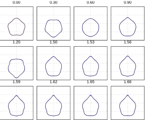
) = constant.For the purpose of verification, we consider an inter- esting example similar to the example introduced by Feng in [13]. In Feng’s example, he is interested in the dynamics of a single drop with charge Q = 0.915Q
(2) R
and initial shape perturbation of the fifth Legendre mode with an amplitude of 0.135. In our example, we consider the case of two drops with a distance of 5 radii between the two centroids. The lower drop posses the same initial conditions as those given in Feng’s example and the upper drop is initially spher- ical and with no charge on it. The generator is par- titioned into 40 quadratic elements (81 nodes) and a time step of ∆t = 0.0001 is used. For compari- son, we overlap the shapes of the lower drop in our case on top of Feng’s result in Figure 2. It seems that the dynamics of the lower drop is very close to that given in Feng’s result till t = 1.65. The sim- ulation in our case, however, stops at t = 1.66 due to the formation of a sharp cusp at the lower drop.The same simulation is repeated with 80 quadratic elements and ∆t = 0.00005 in order to ensure that the formation of cusp is not artificial. Interestingly, the charge distribution of the upper drop is changed by the existence of the lower drop due to Coulomb
attraction. The lower part of the upper drop carries negative charge and the upper part becomes positive.
See Figure 3. Furthermore, the mass conservation of the two drops is within 0.26% and the energy conser- vation of the system is always accurate to the fifth digit. These results clearly established the validity of our numerical calculation.
4 Results
The behaviors of electrostatically coupled droplets are of essential importance in a variety of applica- tions. Theoretical analysis of the dynamics of two droplets under electrostatic interactions is formidable if not impossible. Numerical simulation, however, provides a convenient way of understanding the dy- namics without much difficulties. In this section, ex- tensive but not exhaustive interesting simulations will be presented to illustrate how the deformations of the free surfaces of the two droplets are complicated by the quiescent electrostatic interactions between them.
4.1 Coulomb Attraction
Coulomb attraction between a charged object and other conductors due to charge induction is widely known in electrostatics. However, the coulomb at- traction between a charged droplet and a neutral one has not been studied quantitatively. In the first example, we consider the case of Coulomb attrac- tion between a neutral spherical droplet (upper) with
Q = 0 and an identical droplet (lower) but charged
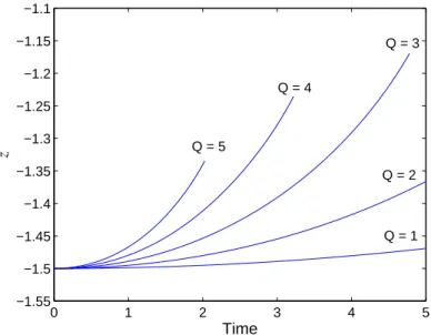
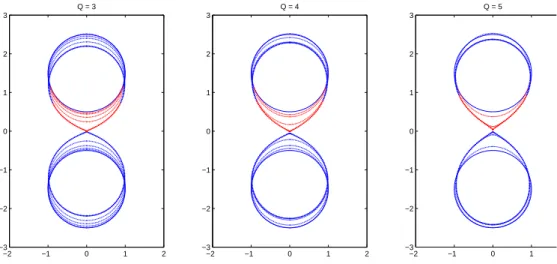
with Q = 1, 2, 3, 4, and 5, respectively. The initial distance between the centroids of the two droplets is 3. The trajectories of the centroids of the lower droplets are plotted in Figure 4. Obviously, the two droplets will move toward and collide with each other eventually. In Figure 5, a few snapshots of the droplets before contact are shown for the cases of Q = 3, 4, 5. The lower part of the upper droplet carries negative charge (in red) and the upper part of the upper droplet becomes positive (in blue) due to charge induction. Similar conical structures form at both droplets at the contact point due to the strongCoulomb attraction resulting from charge induction.
The time histories of the kinetic energy of the lower droplets are shown in Figure 6. The rapid growth of the kinetic energies before contact are related to the local liquid motion associated with Coulomb attrac- tion near the contact point. Our simulations stop im- mediately before the two droplets touch each other.
We may conjecture that the two droplets will coa- lesce into a large droplet and oscillate after charge redistribution but this is beyond the capability of our simulation program.
Next we consider another interesting example in meteorology. It is well known that the cloud droplets formed by condensation nuclei are usually to small to become precipitation. The simplest way of produc- ing precipitation is via the collision and coalescence of small cloud droplets to form large rain droplets.
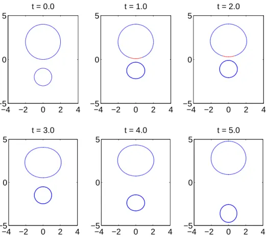
Here we propose to study the coalescence of a small droplet with a large droplet driven by Coulomb at- traction. In this case, the large droplet is assumed to be spherical with R = 3 and neutral while the small droplet is spherical with R = 1 and charge Q = 4.
The initial distance between the centers of the two droplets is 5. See Figure 7. As can be expected, the small droplet is heavily deformed by the Coulomb at- traction and moving toward the large droplet. More interestingly, the deformation of the large droplet is localized at the lower part where the Coulomb at- traction is strong and the surface tension is weak due to the size difference. The upper part of the large droplet is almost stationary.
4.2 Head-on Collision
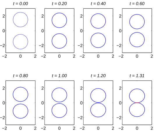
In this example, we consider the cases of two iden- tical spherical droplets with the same charge Q = 4.0 at a distance of 3 radii between the two cen- troids and moving toward each other on a head- on collision trajectory with dimensionless velocity
v = 0.1, 0.3, 0.7, 0.9, and 1.0, respectively. The time
histories of the centroidal position, volume, kinetic energy, surface energy, electrostatic potential of the lower droplet, and total energy of the system are plotted in Figure 8. The dynamics of the upper droplet are similar to those of the lower droplet dueto symmetry. From the time history of volume, we know the mass conservation is excellent. The en- ergy conservation is observed from the time history of the total energy of the system. The electrosta- tic potentials increase at the expense of kinetic en- ergy. In addition, the two droplets will repel each other eventually if the initial velocities are too small (v = 0.1, 0.3, 0.7). Head-on collision is possible only if the two droplets carry sufficiently large initial kinetic energies (v = 0.9, 1.0). Our simulations for head- on collision cases (v = 0.9, 1.0) stopped prematurely when the two droplets touch each other. See Figure 9.
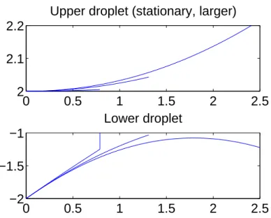
Next, we consider the cases of a small droplet (lower) with radius R = 1, charge Q = 4, and velocity
v = 1 moving toward a large but stationary droplet
(upper) with radius R = 2 and charge Q = 4, 8, 10 along a head-on collision trajectory, respectively. The initial distance between the two centroids is 4. The trajectories of the centroids of the two droplets are plotted in Figure 10. Head-on collisions occur when the large droplet is charged with Q = 4 and 8. When the large droplet carries a charge of Q = 10, the small droplet is reflected after its kinetic energy is exhausted during flight. See Figure 11.4.3 Shape Oscillations
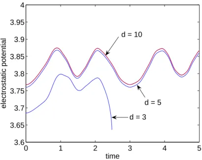
It is interesting to know how the shape oscillations of a droplet will be affected by the electrostatic inter- action from a neighboring droplet. As we have seen from the previous sections, the electrostatic interac- tion is effective only if the two droplets are very close to each other. But how close? Certainly, the dis- tance will depend on the charges carried by the two droplets. As an example, we consider the following cases. The upper droplet is spherical and neutral.
The lower droplet is charged with Q = 4 and sub- ject to a shape perturbation of the second Legendre mode P
2
with a moderate amplitude of 0.4. The dis- tances between the centroids of the droplets are 3, 5, and 10, respectively. The question is how to quantify the electrostatic interaction meaningfully? A simple measure is to compare the electrostatic potential of a single droplet in the universe carrying a charge Q with that of the charged droplet considered in ourcases. See Figure 12. The difference between the electrostatic potential of a single droplet and that of two droplets separating by a distance of 10 is in- discernible. Even at a distance of 5, the difference is quite small. In fact, the shape oscillations of the charged droplet for the cases d = 5, and 10 are almost identical to the shape oscillations of a single droplet since the electrostatic interactions in these cases are negligible. The motions of the droplets for the case of
d = 3 are shown in Figure 13. It is clearly seen that
the shape oscillations of the charged droplet deviates from the Legendre modes severely due to the strong Coulomb attraction.5 Conclusions
The quantitative analysis of the dynamics of two charged conducting droplets under electrostatic in- teraction is completed via numerical simulations. In our simulations, the constancy with time of the vol- ume of the oscillating droplets is accurate to 0.3% and the energy conservation of the whole system is always accurate to the fifth digit. Coalescence of a charged droplet and a neutral one always happens due to the Coulomb attraction resulting from the charged induc- tion. Two droplets carrying the same sign of charges on a head-on collision trajectory will repel each other only if the electrostatic repulsion is strong enough to overcome the kinetic energies of the two droplets. It is found that the electrostatic interaction has only localized effect on the motions of the droplets and it is effective only if the two droplets are very close to each other. Consequently, global analysis based upon Legendre modes may not be appropriate for the study of electrostatic interaction.
More interestingly, charge distribution of a weakly charged droplet may be altered by the induction ef- fect from the nieghboring charged droplet. Conse- quently, the Coulomb attraction is possible between two charged droplets of the same sign.
Acknowledgments
This work was supported by the National Science Council of the Republic of China under grant NSC 93-2212-E-011-037.
Net charge Surface tension s
1
Permittivity e 0 Net charge
Surface tension s
2
2
V
*
= 0 R 1
*
Q 1
*Q 2
*
R 2
*
G :
1*G :
2*r 2
W 2
*:
r 1
W 1
*:
s
*s
*2f
*2= 0
s
*2f
*1= 0
Figure 1: Geometric configuration of the two charged droplets.
0.00 0.30 0.60 0.90
1.20 1.50 1.53 1.56
1.59 1.62 1.65 1.66
Figure 2: Shapes of the lower charged drop with Q = 0.915Q (2) R and initial shape perturbation of the fifth
Legendre mode with an amplitude of 0.135 are overlapped on top of Feng’s result. The upper drop is initially
spherical, neutral, and at a distance of 5 radii away from the lower drop.
−2 0 2
−4
−3
−2
−1 0 1 2 3 4
t = 1.660000
Figure 3: The final shapes of the two drops at t = 1.66. The cusp forms at the north pole of the lower drop. The lower part of the upper drop carries negative charge (in red). The upper part of the upper drop becomes positive (in blue).
0 1 2 3 4 5
−1.55
−1.5
−1.45
−1.4
−1.35
−1.3
−1.25
−1.2
−1.15
−1.1
Time
z Q = 5
Q = 4
Q = 3
Q = 2
Q = 1
Figure 4: Coulomb attraction between a neutral spherical droplet (upper) with Q = 0 and an identical droplet
(lower) but charged with Q = 1, 2, 3, 4, and 5, respectively. The initial distance between the centroids of the
two droplets is 3.
−2 −1 0 1 2
−3
−2
−1 0 1 2 3
Q = 3
−2 −1 0 1 2
−3
−2
−1 0 1 2 3
Q = 4
−2 −1 0 1
−3
−2
−1 0 1 2 3
Q = 5
Figure 5: Coulomb attraction between a neutral spherical droplet (upper) with Q = 0 and an identical
droplet (lower) but charged with Q = 1, 2, 3, 4, 5, respectively. The initial distance between the centroids of
the two droplets is 3. The lower part of the upper droplet carries negative charge (in red) and the upper
part of the upper droplet becomes positive (in blue) due to charge induction.
0 1 2 3 4 5
−0.05 0 0.05 0.1 0.15 0.2 0.25 0.3
Time
Kinetic Energy
Q = 5 Q = 4
Q = 3
Q = 2 Q = 1
Figure 6: Coulomb attraction between a neutral spherical droplet (upper) with Q = 0 and an identical droplet (lower) but charged with Q = 1, 2, 3, 4, and 5, respectively. The initial distance between the centroids of the two droplets is 3. The kinetic energy of the lower droplets are plotted versus time.
−5 −4 −3 −2 −1 0 1 2 3 4 5
−4
−3
−2
−1 0 1 2 3 4 5 6