Abstract
*IEEE 802.11e standard is developed for QoS (Quality of Service) provisioning in WLANs (wireless local area networks). Admission Control is a mechanism that controls stations to be served in WLANs. In practice, evaluation of admission control plays an important role for QoS support. The goal of this paper is to calculate the WLAN delays with ACs (Access Categories). The delay calculation can be used to guarantee the QoS of the VoIP and video streams, which is divided into three parts. One is the propagation delay. Another is the delay that packets queue up in stations or APs (access points). The last is the delay which is taken due to collisions. For VoIP and video streams, the second delay is more important than other two delays. Consequently, here we will focus on the calculation of the second delay. Some simulations and numerical results are provided and discussed in detail.
Experimental results show that the proposed method is more accurate in calculating the delay of packets in WLANs.
Keywords: IEEE 802.11e, QoS, WLANs, admission control, access category.
1. Introduction
IEEE 802.11 WLAN standard is being accepted widely and rapidly for many different environments today [4] [8]. Nowadays, VoIP (voice over IP) and video are also two important applications. To efficiently support VoIP and video applications, QoS (quality of service) mechanism must be provided in WLANs. A standard for supporting QoS in WLANs is 802.11e. QoS is an important attribute of software’s usability. QoS is based on that the experiment user uses the software. In WLAN, QoS has many issues like delay, jitter, channel utilization, effecting, robust, and complex. Our research will focus on the part of delay. Delay is the most critical and easily measured in value.
In 802.11e, applications are divided into four groups [9]. These groups are called ACs (Access category). AC0 is the category with highest priority. VoIP packets belong to AC0. Video packets are in AC1. AC1 has only lower priority than AC0. The others are AC2 and AC3. AC2 is for TCP packets and AC3 is for background
*Jun-Ru Chang is with the Institute of Information Systems and Applications, National Tsing Hua University, Hsinchu, Taiwan.
packets.
What 802.11e do is to provide QoS for AC0 and AC1. These two categories are very sensitive for delay.
802.11e also introduces the admission control to improve the QoS support. Admission control is a mechanism to control the stations to be served by an access point. For example, if there is a station wants to join the BSS (basic service set). Access point should forecast that if this station joins in the BSS would other station’s QoS become worse. If no QoS of stations in this BSS would be lower than the threshold, this station may be accepted.
In other side, this station’s request should be rejected.
Packet delay is a major metric for the QoS of VoIP and video applications. According to this result, access point may determine whether it could accept a station to perform the VoIP or video application. Our goal is to calculate the delay of AC0 and AC1 packets. This delay has three parts. One is the propagation delay and it is the delay that a packet transfers through medium. The second type of delay is queuing delay. When station has a packet to transfer, this packet may group to some AC. Each AC has its queue which holds packets that is waiting to be transferred. Before stations content with each other, four ACs would content with each other first. If the packet does not gain the chance to transfer, it will stay in queue and wait for next contention. The time that the packet stays in queue is queuing delay in this mechanism. Not only packets from stations have queuing delay, but also packets from access points. The queuing delay is much more critical in access point. The last part is the delay caused by collision. Collision time is growing up with the number of station or ACs in BSS. Thus the purpose of this paper is to calculate these three delays. When an AC requires for guaranteeing QoS, the access point may use some parameters to calculate the average delay that if the AC is added in this BSS. Then access point can determine weather the AC can be added or not.
The rest of this paper is organized as follows. We introduce the background of 8802.11e in Section 2. We also show some related research works in this section. In Section 3, we propose an admission control model that calculates the delay to provide QoS in WLAN. Some simulations and numerical results are provided and discussed in Section 4. Finally, the conclusion and future works are presented in Section 5.
2. Background
In this section, we will first introduce 802.11e protocol. We will further review the proposed admission
Delay Analysis of Admission Control Mechanism for Supporting QoS in 802.11e
Ching-Hsun Chen1, Chin-Yu Huang1, Jenn-Wei Lin2, and Jun-Ru Chang*
1Department of Computer Science National Tsing Hua University
Hsinchu, Taiwan
2Department of Computer Science & Information Engineering Fu Jen Catholic University
Taipei, Taiwan
control mechanisms in WLANs. The admission control mechanisms will be divided into two categories:
measurement-based and model-based.
2.1.
802.11e
802.11e is developed for supporting QoS and it proposes two new MAC mechanisms: EDCA (Enhanced distributed channel access) and HCCA (HCF contention-based channel access) [5, 10, 11, 12, 14].
EDCA is a mechanism that all stations content. HCCA is that all station poll. 802.11e also defines some major mechanism. Besides, DLP (direct link protocol) is a mechanism that stations directly link without access point.
Block-ACK is a mechanism that receiver acknowledges a block of packet instead of acknowledging a packet a time.
2.2. Measurement-Based Admission Control In measurement-based admission control, AP will continuously measure the status of network such as throughput or delay. There are some measurement-based admission controls in the literature [4]. The first one is the distributed admission control (DAC) [13, 14]. In this admission control, AP will calculate the budget of each transformation. It will take the statistics of the time which every AC transfers their traffic through medium. And there is a transmission limit for all ACs in each station.
When the budget of the AC is depleted, new AC is not allowed to obtain transmission time.
The second is the two-level protection and guarantee mechanism [15]. This mechanism is based on DAC. There are two level protection methods in this mechanism: the tried-and-known and the early-protection methods. The early- protection is the same as the DAC.
Tried-and-known is a method that the AP measures the quality parameters such as throughput or delay in every beacon interval. If the parameter is below a threshold, the new flow will be killed or rejected. The next is the virtual MAC and virtual source algorithm [2, 12]. In this mechanism, stations and AP simulate the MAC layer.
This algorithm operates virtual packets on the radio channel. This algorithm will calculate its collision rate, and then calculate its throughput or delay.
Threshold-based admission control [6] is another type. In this mechanism, each AC has its own occupied bandwidth, Boccu. And there are two thresholds each of them are Bup and Blow. If Boccu is lower than Blo, this means the occupied bandwidth of this AC is too small.
The priority of this AC will be higher during next period.
If Boccu is greater than Bup, the AC’s occupied bandwidth is too big. At next period, the priority of this AC will get down. At last is Harmonica [16]. This scheme would sample parameters such as drop rate, delay, throughput periodically. It also has two algorithms that are employed to select the channel access parameters which best match the QoS requirement. One algorithm is to adjust the differences of different classes which need QoS guarantee.
The other is to adapt the channel access parameters of all the classes to achieve high channel utilization.
2.3. Model-Based Admission Control
Model-based admission controls construct certain performance metrics to evaluate the status of the network [4]. Here are some model-based admission controls. First is Markov chain model-based admission control [3, 11].
In this scheme, admission control predicts the throughput of each flow. The equation is given by
s s idle
c c
si
i P T P aSlotTime P T
P E S P
× +
× +
×
= × [ ]
, (1) where Psi is the probability that the flow i successfully transmits the packet, Pc is the probability of collision, Pidle is the overall idle probability, Ps is the overall successful probability, Tc is the collision time, and Ts is the successful time. Note that E[P] is the data payload.
This admission control mechanism will use the equation to predict the throughput of each flow and determine weather a new flow needs to be accepted or rejected.
Another is the contention-window-based admission control [1]. This mechanism uses contention windows size (CW) of each flow to calculate the throughput. When a new flow wants to join into the network, this mechanism would calculate the throughput that if the new flow has joined in. It uses a model with the parameter of CW. If the resulting throughput can not meet the requirement of QoS, the new flow would be rejected. On the other hand, the flow would be accepted.
3. Proposed Delay Model
Firstly, for admission control of the WLAN, we should calculate the delay each packets for QoS support.
However, the previous measurement-based and model-based admission control mechanisms do not concern the delay metric. In infrastructure BSS, there are downlink from AP and uplink from station. These delays may be an important result of QoS. If an AC wants to add in the BSS, access point will calculate how the new AC will affect the delay in this network. If the delay is longer than the service can stand for, this AC will be reject. In other way, the AC will be accepted.
3.1 Propagation Delay
Propagation delay means the delay of a packet transmitting. In EDCA, before counter starting backoff, AC should wait a time that is called AIFS [AC]. Each AC has its own AIFS [AC]. This value may be modified in different case. But there are some attributes may be the same. AC0 for VoIP may have the shortest AIFS, in other words AIFS [AC0] is the shortest AIFS of all. In DCF, DIFS is SIFS plus 2 times of AIFS slot time. AIFS should not shorter than DIFS. So the AIFS may be the sum of SIFS and 3 or more times of AIFS slot time. After AIFS [AC], the counter of AC starts backoff. The backoff time depends on CW. Backoff time (Tbackoff) is a random value between 0 and CW. If CW is large, it may means there is higher priority that AC’s backoff time gets longer.
CWmax and CWmin determine the CW. CW may be
CWmin at first. If this AC collides with other AC, CW will be two times larger until it reaches the CWmax. After backoff time, if the medium is not in use, AC could transfer its packet immediately. Transformation through medium may also cause some delay. This delay is defined as Ttran. The sum of these delays may be the delay of propagation delay. This can be shown as the following equation:
tran backoff n
propagatio AIFS AC T T
Delay = [ ]+ + . (2)
3.2 Queuing Delay
Queuing delay means the delay of a packet that stays in station or access point’s queue. We calculate this kind of delay as that the time of that other station’s transmission is completed. Every packet has its own propagation delay. But when transformation is completed, it should also consider about the delay of ACK. In EDCA, after transmitting a frame, receiver will wait a SIFS and then send ACK to sender. In queuing delay, the ACK time should be took into account. This may be calculated by the following equation:
ACK SIFS
T T
AC AIFS
DelayN queue backoff tran +
+
+ +
= [ ] . (3)
Each successfully transferred packet may cost DelayNqueue. A packet may stay in queue between 0 to AC number multiply DelayNqueue. On average, we can calculate that the packet is transferred as the medium of all ACs in every mobile node. In other words, there are half of the numbers of AC (NumberAC) packets transfer before this packet. Consequently, we have
queue AC
queue Number DelayN
Delay =( /2)× . (4)
3.3 Collision Delay
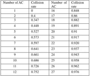
When two or more stations send frames at the same time, collision occurs. Not only in WLAN but also in wired LAN, collision is a big problem. In this paper, we do not use model to figure the collision out. Instead, we use some values that from experiments, given in Table 1.
Table 1. Collision rate from experiment for CWmin = 7 and CWmax = 15
Number of AC Collision rate
Number of AC
Collision rate
1 0 16 0.848 2 0.4 17 0.86 3 0.347 18 0.882 4 0.448 19 0.891 5 0.527 20 0.91 6 0.573 21 0.917 7 0.597 22 0.920 8 0.641 23 0.937 9 0.661 24 0.943 10 0.686 25 0.958 11 0.726 26 0.962 12 0.752 27 0.976
13 0.798 28 0.979 14 0.817 29 0.982 15 0.833 30 0.984
This table’s value can be verified by [3]. In [3], the probability of collision is calculated by Markov chain. In this model, calculating the collision probability is minute and complicated. But we can use the model to verify our experiments values. By using this model, we put these to verify if these values ate reasonable. And the result is good; the error rate is less than 5%.
The collision delay for a packet may be calculated as the product of collision times and Timetran. But the collision rate means the total transmission times divide the collision times. The equation is shown as follows:
tran collision
collision
collsion Time
Rate
DelayN Rate ×
= − 1
. (5) For a packet, the collision delay for it is DelayNcollision. But this is not enough. Considering about queuing delay, collision may occur to every collision in each transformation. So the delay that caused by collision should consider about the delay that the packet occurs collision which is transferred earlier than this packet. We can calculate it as the half of the AC number. The equation can be obtained as
collision AC
collision Number DelayN
Delay = /2× . (6) 3.4 Uplink and Downlink Streams
In VoIP, there are two streams, one is uplink, and another is downlink. Uplink streams means that the frame sending from station to AP. Most of these packets carry user’s data from station to AP. In the most popular application of VoIP, Skype, it may send frames in a fixed time. Even if user does not speak, Skype would also send a packet to AP. If there are some data need to be transferred to AP, the packet may be larger. Downlink is similar to uplink. Downlink streams are the packets from AP to stations. The downlink packet may come from another station or other user in different BSS. In other words, these downlink packets may be uplink packets for that station or user. Video application is another AC that is should guaranteed QoS. But in video, downlink is much more important than uplink. When user watches video online, most data packets are from AP. Station may not send many frames to AP. In most video, station and AP may use UDP to transmit frames. In UDP, receiver does not need to send ACK to sender. In video application, we can only consider the downlink from AP.
3.5 Admission Control Analysis
To consider the admission control of the BSS, first we should define what admission control is. Admission control is an algorithm to ensure that admittance of a new flow into a resource constrained network does not violate parameterized service commitments made by the certain priorities [7]. In other words, before a new AC gets into a BSS, admission control mechanism should project how
this new AC will affect the QoS of the BSS. In our mechanism, the above three delays will be calculated as the flag of QoS. In uplink case, every packet’s delay given by
collisoion queue
n propagatio
uplink Delay Delay Delay
Delay = + + .
(7) The delay of uplink may be the simple sum of these three delays. Before a packet transfer, it should stay in queue. The time that the packet stays in queue is the queuing delay. When the packet starts transformation, the time that it cost to arrive AP is the propagation delay. If there is occurred collision during transmission time, the time that is wasted is called collision delay. The delay can be calculated as these three delays.
In downlink streams, there is some little different.
In uplink streams, an AC may have one packet a time.
But downlink streams in AP are very different. Every VoIP application may have one uplink and one downlink.
For this reason, AC may have the number of stations of downlink packet a time. So, the delay of downlink may be larger than uplink. Not only may the load of AC make the packet delays. In EDCA, AP should content with other stations. In short, the TXOP of AC should share every packet in queue. In other words, before a packet transfers to receiver, it should stay in queue until the packet that comes in queue earlier. If there is N ACs which supports QoS in BSS, AC may receive N downlink packet a time. if the packet wants to be transferred, it may wait for N/2 packets in average. But AP may contents with other stations. So AP may wait N/2 stations transferring their packets. The queuing delay of downlink may be N2/4 times of the DelayNqueue. The collision delay has the same problem. Because every packet may occur collision, the transmission times before this packet transfer is N/2 times than uplink. In other words, the collision delay of downlink is N2/4 times of DelayNcollision. The equation of downlink delay is given by
collision AC
queue
AC n
propagatio downlink
DelayN Number
DelayN
Number Delay
Delay
4
4
2
2
+
×
+
= . (8)
But this equation is not very suited for most case.
This equation assumes every AC has a packet in a very short time. In most case, the time interval is not as short as packet transmission time. So in most case, there are not as many packets as N2. If the time interval is longer than the time that all packets have transferred, the packet number in downlink may be 2N instead of N2. Thus we have
collision AC
queue
AC n
propagatio downlink
DelayN Number
DelayN
Number Delay
Delay
× +
×
+
= . (9)
In this mechanism, downlink is the bottleneck of the QoS. Because the propagation delay is very small, the growth of downlink delay may be larger than that in uplink. It is almost two times. In admission control, if downlink can not reach the target of QoS. This BSS may not reach the quality. In other words, AP may detect downlink delay to determine weather the AC can join in
the BSS.
If the is a new AC wants to join in the network, we will calculate the delay of the BSS that if the new AC has joined in using Equation 9 firstly. And find out that if the delay which is larger than the half of the time interval between two packets. In the case of that the delay is larger, when packets enter into the queue of AP, there may be some packets that come at the previous period not transferred. This may cause the jam in AP’s queue. And the Equation 9 is not suited in this case. There are not only 2N packets at the head of it. We should use N2 instead of N to calculate the delay. According to those two results, we may determine that if the new AC is allowed joining into the BSS.
Only considering about the downlink streams has some advantages. Because the parameter is from AP, AP can calculate the delay without getting information from stations. Then without calculating uplink delay, AP can reduce the calculation. At last, in video streams only has downlink packet, so calculation of these delays may be much easier implemented in practice.
4. Evaluations
4.1. Simulation Environment
To validate the proposed delay model of the admission control, we also perform simulation experimenters. In simulation experiments, we use NS-2 (version 2.28) [17] with an 802.11e module [18] to simulate the traffic of the WLAN. The PHY layer is 802.11g.
In the simulation environment, there are 30 wired VoIP node, a gateway, an AP, and 30 wireless stations.
Wired VoIP devices connect to the gateway with wired network which has the data rate of 100Mbps and propagation delay of 5ms. The gateway connects to AP with wired network which has the data rate 100Mbps and propagation delay of 2ms. Wireless stations connect to AP.
These stations have an error model to simulate the real environment. We set it to 10%. And each station has a random movement. The environment is shown in Figure 1. Besides, some parameters are given Tables 2 and 3.
100Mpbs 2μs
Wireless STA AP Gateway Wired VoIP Device
100Mpbs 5ms 6Mpbs/
54Mbps
Figure 1. Simulation configuration
In the scenario, downlink and uplink will send a packet of 200 bits. The time interval that is between two packets is 20 milliseconds. At the first second, the first station starts transformation and the first wired mobile device also starts transformation. At the second, the second station and mobile device start transformation.
And so on, until there are 30 traffics in BSS. The environment will record the packet until 40 seconds.
Table 2. 802.11e parameters
AC PF AIFS CW_MIN CW_MAX TXOPLimit voice 2 2 7 15 0.003008 video 2 2 15 31 0.006016 best effort 2 3 31 1023 0
background 2 7 31 1023 0
Table 3. 802.11g parameters
Parameters Value CWmin 15 CWmax 1023 Slot time 9us
CCA time 4us Rx Tx turnaround time 5us
SIFS 10us Preamble length 144 bits
PLCP header length 48 bits PLCP data rate 6Mbps Max propagation delay 4us
4.2. Simulation Results Analysis
We use some static tools to gather the statistics of the delay. In every time slot as 1 second, we calculate the delay time of every downlink packet. And we would get the result as the average delay of packets that is transformed in this second. Table 4 gives the simulation results.
The threshold of VoIP is about 100 milliseconds.
We can obtain that if there are 15 ACs in BSS the delay may over 100 milliseconds. In other words, this BSS can only have 14 or less VoIP ACs. This result also shows some other interesting characteristics. It is more rapidly from 14 to 15.Delay form 14 to 15 almost grows 147 milliseconds. The reason of this result may be that the collision effect is more critical in this time period.
Because the CWmax is 15, the collision rate of this period may grow rapidly. And another reason is the queue in AP is overloading.
Table 4.Downlink delay
Time (s)
Delay (ms)
Time (s)
Delay (ms)
Time (s)
Delay (ms) 1 0.3688 11 4.69780 21 1076.84773 2 0.58547 12 5.82571 22 953.90986 3 0.86871 13 8.93151 23 1139.79861 4 1.15521 14 33.62407 24 1297.78777 5 1.42094 15 150.59357 25 1101.31068 6 1.68852 16 252.05898 26 1402.97829 7 2.15044 17 438.13009 27 1199.45188 8 2.39243 18 769.61506 28 1391.90152 9 2.8681 19 901.92672 29 1611.22768 10 3.97099 20 1087.71964 30 1476.60914
4.3. Admission Control Analysis
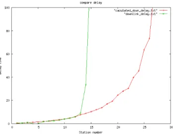
We use Equation 9 to calculate the delay in this environment. The result is given in Table 5. The comparison result is plotted in Figure 2.
Figure 2. Comparison results
Before the 13th second, the calculated result is similar to the simulation result. But in the 15th second, calculated result has a big different from simulation result.
The reason is at the 15th second, there are 15 ACs in BSS.
And its delay is 10.3 milliseconds. In this environment, AC will get packets every 20 milliseconds. The average delay of each packet is 10.3 milliseconds, so the longest delay of all may be two times of average. The delay is about 20.6 milliseconds. This delay is longer than 20 milliseconds, and the queue may be overloading. In other words, when some new packets enter to the AP’s queue, there may be a traffic jam in AP because the packet that comes at previous period may not be transferred yet. In this case, we may calculate the delay with N2 packets.
The result is about 152 milliseconds. This is over the delay limit of 100 milliseconds. And our result also shows that if there are 15 ACs in the BSS, AP’s downlink queue will be overloading. This may let packets dropped.
So we may not let the 15th AC join into the BSS.
Table 5. calculated delay of Equation. 9
Time (s) Delay (ms) Time (s) Delay (ms) 1 0.308 16 11.971 2 0.602 17 13.771 3 0.783 18 16.986 4 1.110 19 19.438 5 1.509 20 24.444 6 1.921 21 27.902 7 2.320 22 30.277 8 2.887 23 39.658 9 3.384 24 45.382 10 3.985 25 63.518 11 4.902 26 73.374 12 5.813 27 118.533 13 7.563 28 141.592 14 8.874 29 168.965 15 10.340 30 201.421
5. Conclusions
In this paper, we propose a model-based admission control mechanism for calculating the delay of packets which belongs QoS supported ACs. In the propsoed mechanism, we calculate three types of delay. The average delay is calculated by the simple sum of these three delays. Access point may determine weather a station is able to be added in BSS according to this average delay. First is propagation delay. This type of delay depends on the PHY layer and MAC setting of BSS.
Propagation delay will calculate the delay for packet transferring through medium and backoff time. The second type is the most critical delay of these three. This type is queuing delay. This type delay is that a packet stays in queue. A packet would be transferred only that the packet which gets into the queue earlier has been transferred. The delay of a packet is successfully transferred contains transferring time, DIFS, SIFS, backoff time, and ACK. These parameters may be different in different PHY layer. Queuing delay can be calculated by the sum of propagation delay multiplying the square of station number. The third type is collision delay. This kind of delay is calculate by collision rate multiply transfer time. In this paper we use the value from experiment for the collision rate.
VoIP has uplink and downlink and video has only downlink. The downlink of access point becomes the bottleneck of the QoS. Because each VoIP AC has it own downlink. The queue in the access point grows much faster than stations. Video is very like VoIP. Finally, we use the NS-2 tools with 802.11e module to simulate our approach mechanism. In our simulation, the delays are close to our calculation before the BSS is overload. In our simulation environment, 15 ACs with QoS support reach the threshold. VoIP can accept the delay of 100 milliseconds. In our simulation result, in the case of 15 AC0s the delay grows to 150 milliseconds. And our calculation result before 15 stations is close to the result of simulation. In short, our admission control mechanism will reject ACs joining in the BSS if there are more than 15 ACs in BSS.
Acknowledgment
The work described in this paper was supported by the National Science Council, Taiwan, under Grant NSC 96-2221-E-007-079, and by a grant from the Ministry of Economic Affairs (MOEA) of Taiwan (Project No. 95- EC-17-A-01-S1-038).
References
[1] A. Banchs, X. Perez-Costa, and D. Qiao, “Providing Throughput Guarantees in IEEE 802.11e Wireless LANs,” Proceedings of the 18th. International Teletraffic Congress (ITC-18), Berlin, Germany, Sept. 2003, pp.
1001–10.
[2] M. Barry, A. T. Campbell, and A. Veres, “Distributed Control Algorithms for Service Differentiation in
Wireless Packet Networks,” Proceedings of the IEEE Conference on Computer Communications (INFOCOM 2001), vol. 1, Anchorage, AK, 2001, pp. 582–90.
[3] G. Bianchi “Performance Analysis of the IEEE 802.11 Distributed Coordination Function,” IEEE Journal on Selected Areas in Communications (JSAC), vol. 18, no. 3, Mar. 2000, pp. 535-48.
[4] D. Gao and J. Cai, “Admission Control in IEEE 802.11e Wireless LANs,” IEEE Network, July/August 2005, pp 6-13.
[5] A. Grilo, M. Macedo, and M. Nunes, “A Scheduling Algorithm for QoS Support in IEEE 802.11e Networks,”
IEEE Wireless Commun., vol. 10, no. , June 2003, pp.
36–43.
[6] D. GU and J. Zhang, “A New Measurement-Based Admission Control Method for IEEE802.11 Wireless Local Area Networks,” Technical report TR-2003-122, Mitsubishi Elec. Research Lab., Oct. 2003.
[7] C. Heegard, J. Coffey, S. Gummadi, P. Murphy, R.
Provencio, E. J. Rossin, S. Schrum, and M. B. Shoemake
“High-Performance Wireless Ethernet”, IEEE Communication Magazine, vol. 39, no .11, Nov. 2001.
[8] IEEE Std. 802.11, “Wireless LAN Medium Access Control (MAC) and Physical Layer (PHY) Specifications,” 1999.
[9] IEEE Std. 802.1D, “Media Access Control (MAC) Bridges,” 2004.
[10] IEEE P802.11e/D6.0, “Wireless Medium Access Control (MAC) and Physical Layer (PHY) Specifications:
Medum Access Control (MAC) Quality of Service (QoS) Enhancements,” Nov. 2003.
[11] D. Pong and T. Moors, “Call Admission Control for IEEE 802.11 Contention Access Mechanism,” Proceedings of IEEE GLOBECOM’03, vol. 1, San Francisco, CA, Dec.
2003, pp. 174–78.
[12] A. Veres et al., “Supporting Service Differentiation in Wireless Packet Networks Using Distributed Control,”
IEEE Journal on Selected Areas in Communications (JSAC), vol. 19, no. 10, 2001, pp. 2081–93.
[13] Y. Xiao and H. Li, “Evaluation of Distributed Admission Control for the IEEE 802.11e EDCA,” IEEE Communication Magazine, vol. 42, no. 9, 2004, pp.
S20–S24.
[14] Y. Xiao and H. Li, “Voice and Video Transmissions with Global Data Parameter Control for the IEEE 802.11e Enhance Distributed Channel Access,” IEEE Transactions on Parallel and Distributed Systems, vol. 15, no. 11, 2004, pp. 1041–53.
[15] Y. Xiao, H. Li, and S. Choi, “Protection and Guarantee for Voice and Video Traffic in IEEE 802.11e Wireless LANs,” Proceedings of the IEEE Conference on Computer Communications (INFOCOM 2004), vol. 3, Hong Kong, Mar. 2004, pp. 2152–62.
[16] L. Zhang and S. Zeadally, “HARMONICA: Enhanced QoS Support with Admission Control for IEEE 802.11 Contention-based Access,” Proceedings of the 10th IEEE Real-Time and Embedded Technology and Applications Symposium (RTAS 2004), Toronto, Canada, May 2004, pp.
64-71.
[17] http://www.isi.edu/nsnam/ns/, Information Sciences Institute, University of Southern California, 7/18 2006.
[18] http://www.tkn.tu-berlin.de/research/802.11e_ns2/,Teleco mmunication Networks Group, 7/18 2006.