Efficient parallel algorithms for doubly convex-bipartite graphs

(1)

ELSEVIER Theoretical Computer Science 147 (1995) 249-265

Theoretical Computer Science

Efficient parallel algorithms for doubly convex-bipartite

graphs *

Chang-Wu Yu, Gen-Huey Chen*

Department of Computer Science and Information Engineering, National Taiwan University, Taipei, Taiwan

Received August 1992; revised May 1994 Communicated by M.S. Paterson

Abstract

Suppose that G = (S, T,E) is a bipartite graph. An ordering of S(T) has the adjacency property if for each vertex in T(S), its adjacent vertices in S(T) are consecutive in the ordering. If there exist orderings of S and T which have the adjacency property, G is called a doubly convex-bipartite graph. In this paper, a parallel algorithm is proposed to recognize a doubly convex-bipartite graph. The algorithm runs in O(log n) time using O(n3/log n) processors on the CRCW PRAM, or O(log’ n) time using O(n3/log2 n) processors on the CREW PRAM.

1. Introduction

An undirected graph G with vertices (ul, u2, . . . , u,} is called a permutation graph [lo] if there exists a permutation 7c on N = { 1,2, . . . , n} such that for all i, jEN,

(i - j)(n-‘(i) - n-l(j)) < 0

if and only if Ui and uj are joined by an edge in G. Pictorially, draw the vertices

Ul,U2, -.*, u, in order on a line, and v+(~), v,(~), . . . . u,(,) on a parallel line such that for

each iEN, Vi is directly above U,(i). Next, for each &N, draw a line segment from Vi on the upper line to Ui on the lower line. Then, there is an edge (Ui,Vj) in G if and only if the line segment for Ui intersects the line segment for Uj. As an illustrative example, Fig. 1 shows a permutation 7~ = (4,7,5,1,2,6,3) and its corresponding permutation graph.

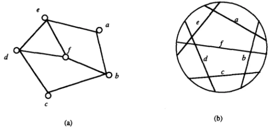
An undirected graph G is called a circle graph [SO] if there exists a set C of chords on a circle and a l-l correspondence between C and the set of vertices of G such that two vertices are adjacent in G if and only if their corresponding chords intersect. The

*This research is supported by the National Science Council of the Republic of China with the grant NSC82-0408-E-002-409.

*Corresponding author. E-mail: [email protected].

(2)

250

i:

z(i) :

C.-W. Yu, G.-H. Chen J Theoretical Computer Science I47 (1995) 249- 265

4 i’ 5 1 2 6 3

(a) (b)

Fig. 1. An example. (a) A permutation 1~. (b) Its corresponding permutation graph.

e

d

b

c

(a) (b)

Fig. 2. An example. (a) A circle graph. (b) One of its circle-graph models.

set C is called a circle-graph model for G. Fig. 2 shows a circle graph along with one of its circle-graph models.

A bipartite graph is a graph whose vertex set can be partitioned into two subsets S and T such that each of its edges has one end in S and the other end in T.

A permutation graph which is also bipartite is called a bipartite-permutation graph.

A circle graph which is also bipartite is called a bipartite-circle graph.

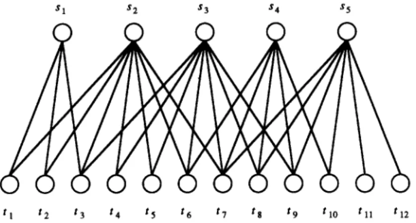
Let G = (S, T, E) denote a bipartite graph, where S u T is the set of vertices and E is the set of edges. Also, let N(o) denote the set of vertices which are adjacent to u in G. An ordering of S(T) has the adjacency property if for each vertex oeT(S), N(o) contains consecutive vertices in an ordering. An ordering of S(T) has the enclosure

(3)

C.-W. Yu, G.-H. Chen / Theoretical Computer Science 147 (1995) 249- 265 251

tl t2 t3 t4 t5 ‘6 t7 tE ‘9 t 10 t11 * 12

Fig. 3. An ordering of S and an ordering of T which have the adjacency and the enclosure properties.

N(t,) contains consecutive vertices in the ordering. See Fig. 3, where an example is shown. The combination of an ordering of S and an ordering of T is called a strong

ordering if any two edges (sip tl), (sj, t&E imply (si, tk)~E and (sj, tl)~E, where si, sjES> tk, try T, Si precedes sj in the ordering of S, and tk precedes tl in the ordering of T. To make the definition clearer, let us imagine the vertices of S: s1 , s2, . . . , slsl arranged on

a line and the vertices of T: tI, t2, . . . . tlTl on a parallel line. They form a strong ordering if for all si, sjES, tk, try T (i < j and k < I), (Si, tk) and (sj, tJ exist whenever (si, tr) and (sj, tk) cross. The combination of the ordering of S and the ordering of

T shown in Fig. 3 forms a strong ordering.

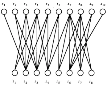
The graph G = (S, T, E) is called a conoex-bipartite graph if there are orderings of S or T having the adjacency property, and a doubly convex-bipartite graph if there are orderings of S and T having the adjacency property [12]. See Fig. 4, where a doubly convex-bipartite graph is shown.

Glover [9] showed a practically important application of doubly convex-bipartite graphs in industry. Lipski and Preparata [12] solved the maximum matching problem on both doubly convex-bipartite graphs and convex-bipartite graphs. Dekel and Sahni [6] developed an efficient parallel algorithm that finds maximum matchings in convex-bipartite graphs. Their result may also be used to solve several scheduling problems.

As we will see later in this paper, bipartite-permutation graphs are a subclass of doubly convex-bipartite graphs, which are a subclass of bipartite-circle graphs. Spinrad et al. [14] presented an O(m + n) time recognition algorithm for bipartite- permutation graphs, where n and m are numbers of vertices and edges, respectively. Chen and Yesha [3] presented a parallel algorithm that recognizes a bipartite- permutation graph in 0(log2 n) time using 0(n3) processors on the CRCW PRAM (concurrent-read concurrent-write parallel random access machine). Recently, Yu and Chen [16] improved the work of Chen and Yesha by presenting a parallel algorithm that runs in O(logn) time using O(n3/logn) processors on the CRCW PRAM or

(4)

252 C-W. Yu, G.-H. Chen 1 Theoretical Computer Science 147 (199.5) 249- 265

Sl s2 s3 s4 ss ‘6 Sl sa s9 SlO

t1 t2 t3 t4 t5 ‘6 t7 ta

Fig. 4. A doubly convex-bipartite graph.

O(logz n) time using 0(n3/log2 n) processors on the CREW PRAM (concurrent-read exclusive-write parallel random access machine).

Testing for the consecutive l’s property for a (0, l)-matrix is an important problem. Given a (0, 1)-matrix, this problem asks whether it is possible to permute its columns so that there are consecutive l’s in each of its rows. If it is so, we are also interested in knowing how the columns should be permuted. The problem has applications in many fields such as genetics, archaeology, information science, operations research, and so on [2]. Klein and Reif [l l] show that this problem can be solved in O(log3 n) time using O(n2) processors on the CREW PRAM, as a result of parallel algorithms for PQ-trees. Recently, Chen and Yesha [2] further reduced the time complexity to O(log’ n) time by using 0(n3) processors on the CRCW PRAM. With slight modifica- tions, the algorithm of Chen and Yesha can recognize convex-bipartite graphs (and therefore doubly convex-bipartite graphs) with the same time complexity and processor complexity.

In this paper, we show that for the purpose of recognizing doubly convex-bipartite graphs, there exist faster algorithms requiring fewer processors than that of Chen and Yesha. We present a parallel algorithm that recognizes a doubly convex-bipartite graph in O(logn) time using O(n3/logn) processors on the CRCW PRAM or O(log’ n) time using 0(n3/log2 n) processors on the CREW PRAM. Compared with the result of Chen and Yesha [2], our algorithms need less time and fewer processors on the same computation model, or the same time but fewer processors on a weaker model.

The rest of this paper is organized as follows. In the next section, we introduce some properties about doubly convex-bipartite graphs, which form the basis of our algorithms. In Section 3, we present a parallel algorithm for recognizing doubly convex- bipartite graphs. In Section 4, we conclude the paper with some final remarks.

(5)

C.-W. Yu, G.-H. Chen / Theoretical Computer Science 147 (1995) 249-265 253

2. Properties

Before introducing properties of doubly convex-bipartite graphs, we first give some necessary definitions and notations.

The complement of a graph G is a graph having the same vertex set as G, whose any two vertices are adjacent if and only if they are not adjacent in G. For a bipartite graph G = (S, T, E), we define a graph G& whose vertex set is S and whose edge set is defined as follows: for all sip sjES, (sr, sj) is an edge of G ;, r if and only if N(si) E N(sj) in G. Suppose that U and Vare nonempty subsets of S and T, respectively. The subgraph of G whose vertex set is U u V and whose edge set contains those edges of G that have both ends in U u V is called the subgraph of G induced by U and V, and is denoted by Gu,v.

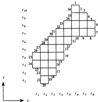
Suppoose that G = (S, T, E) is a bipartite graph, and sl, s2, . . . , slsl and tr , t2, . . . , tl TI are orderings of S and T, respectively, having the adjacency property. Then G can be expressed as a rectilinear polygon: we only need to place a square at the position (ti, sj) for each edge (sj,ti)EE. The polygon has a shape like Fig. 5 or its reflection with respect to a vertical line. Without loss of generality, we consider the polygon looks like Fig. 5 in the rest of this paper. As we will see later, many of the properties introduced in this section become clearer by the aid of the polygon.

As a consequence of the adjacency properties of S and T, there are two structural properties about the polygon: (1) each row (column) of the polygon contains a

s 10 59 S8 Sl S6 $5 s4 s3 s2 SI 6 I 25 24 tl r2 t3 ‘4 ‘5 ‘6 ‘7 ‘8 x

(6)

254 C.-W. Yu, G.-H. Chen / Theoretical Computer Science 147 (1995) 249- 265

continuous block of squares; (2) the right (left) boundary of the polygon consists of two portions: one is nondecreasing and the other is nonincreasing from bottom to top. Intuitively, each row and each column of the polygon represent a vertex in S and a vertex in T, respectively, and the specified square represents an edge connecting the two vertices.

A row is maximal if there exists no row that can properly cover it. For example, rows s4,sg,s7 in Fig. 5 are IEiXiId. A row iS right mUXimd (kf maximal) if it k

maximal and has the greatest (smallest) x-coordinate. If more than one candidate exists, select the uppermost (lowest) one as the right (left) maximal row. For example, row s7 is right maximal and row s4 is left maximal.

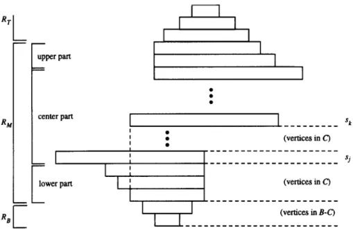
The polygon can be partitioned into three parts: bottom region (Ra), middle region (&), and top region (Rr). The middle region consists of three parts: upper part, center part, and lower part, which are separated by the right and left maximal rows. The upper part contains those rows above the right maximal row whose leftmost squares have the same x-coordinate as the right maximal row. The lower part contains those rows below the left maximal row whose rightmost squares have the same x-coordinate as the left maximal row. The right maximal row, the left maximal row, and those between them constitute the center part. For example, see Fig. 5 where the center part contains rows s4, ss, s6, s7. No upper part and lower part exists in this example. The rows above the middle region constitute the top region, and the rows below the middle region constitute the bottom region. See Fig. 5 where the top region contains rows s8,s9,slo and the bottom region contains rows s1,sz,s3.

In the following, we introduce sets A and C of rows which will be mentioned very often in the subsequent discussion. The set A contains all the maximal rows. The set C contains the rows of the middle region with the removal of maximal rows.

Definition 1. Suppose that sl,sz, . . . . slsl and tr, tz, . . . . tlrl are orderings of S and T,

respectively. We define the following notations. p(si) = min { j 1 tjEiV(S~)}e q(Si) = max(jI tj~l\r(si)}. A = {siIsiES and there does not exist SjES such that N(q) is a proper subset of N(sj)}. B = S - A. C = {si 1 SiEB and one of the following two conditions holds: (1) there exists exactly one vertex SjEA and there exists another vertex SHEA such that N(si) is a proper subset of N(sj), N(sj) A N(s~) # 8, and N(sj) n N(s,J E N(si); (2) there exist exactly two vertices sj, QEA(J’ # k) such that N(sj) n N(s~) = N(q) and N(q) is a proper subset of N(sj) and N(Q)}.

Forexample,A= {s4,ss,s7),B= {s s s s s s s },andC= 1, 2, 3, 5, 8, 9, 10 {ss}forFig. 5. A further explanation of sets A,B, C is given in Fig. 6. It also provides a further explanation of the top, middle, and bottom regions.

Throughout this section, unless mentioned particularly, we assume that G = (S, T, E) is connected and N(si) # N(sj) for all si, Sj~S, si # sj. The following two lemmas state basic properties of the rectilinear polygon. Since they are clear by observing the rectilinear polygon, their proof is omitted.

(7)

C-W. Yu, G.-H. Chen 1 Theoretical Computer Science 147 (1995) 249- 265 255 RT

L

I I

I

I-

1

I upper Part I . . . Rk4

I

center part

L

~_________

. ______-_-_----_--

.

‘k

FweF____________-_%_

‘j -I - _____________________ RB

c

I

(vertices in B-C)

____________________---

Fig. 6. A further explanation of sets A, B, C, where sj (s,J is the first (second) vertex in A.

Lemma 1. Suppose

RM= AvC.

that G = (S, T, E) is a doubly convex-bipartite graph. Then,

Lemma 2. Suppose that G = (S, T, E) is a doubly convex-bipartite graph. Then, for all

si,sj, where si,sjERT or si,sjERB, we have N(si) s N(sj) or N(sj) c N(si).

Lemma 3. Zf G = (S, T, E) is a doubly convex-bipartite graph, then G is a bipartite-

circle graph.

Proof. We show that G is a bipartite-circle graph by constructing one of its circle- graph models. Suppose that sl,sz, . . . . slsl and tl, t2 , . .., tlTI are orderings of S and T,

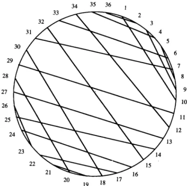
respectively, which have the adjacency property. We first construct a rectilinear polygon from G by placing a square at the point (ti,Sj) for each edge (Sj, ti)EE. The rectilinear polygon has a shape like Fig. 5 or its reflection with respect to a vertical line. Then, we traverse the boundary of the polygon clockwise (starting at any edge), and label the edges with numbers from 1 to 2( IS/ + 1 T I). Finally, we arrange these numbers around a circle, and generate a chord joining i and j if they are on the same row or on the same column in the rectilinear polygon (see Fig. 7). It is easy to see that the set of chords represents a circle-graph model for G. So, G is a bipartite-circle graph. 0

(8)

256 C.-W. Yu, G.-H. Chen J Theoretical Computer Science 147 (1995) 249-265

Fig. 7. A circle-graph model for the double convex-bipartite graph of Fig. 4.

Lemma 4. For each vertex sieB, there exists a vertex sjeA such that N(q) is a proper

subset of N(Sj).

Lemma 5. Suppose that G = (S, T, E) is a bipartite graph. Then, GA,T is connected. Proof. Suppose that GA. r is disconnected and contains r > 1 connected components. Therefore, T can be partitioned into TI, T2, . . ., T, each of which is contained in one component of GA,r. Then for each vertex s,EB, we have N(q) E Tk for some k,

1 < k < r (if this is not true, then there exists a vertex s+B such that N(s*) is distributed over at least two subsets of T, which is in contradiction to Lemma 4). However, this implies that G is also disconnected, which is a contradiction. •!

Lemma 6 (Spinrad et al. [ 14, Theorem l] ). Thefollowing statements are equivalent for

a bipartite graph G = (S, T,E).

(1) G is a bipartite-permutation graph. (2) There is a strong ordering of S and T.

(3) There exists an ordering of S (or T) which has the adjacency and enclosure properties.

Note that the ordering of S and the ordering of T, which form a strong ordering, mentioned in statement (2) of Lemma 6 have the adjacency and enclosure properties,

(9)

C.-W. Yu, G.-H. Chen / Theoretical Computer Science I47 (1995) 249-265 251

provided G is connected. This can be seen from the proof of Theorem 1 in [14] and is stated as the following lemma.

Lemma 7. Suppose that G = (S, T, E) is a bipartite graph and there exists a strong

ordering of S and T. Then, the ordering of S and the ordering of T, which form the strong ordering, have the adjacency and enclosure properties.

Lemmas 6 and 7 imply that bipartite-permutation graphs are a subclass of doubly convex-bipartite graphs.

Lemma 8. Suppose that G = (S, T, E) is a doubly convex-bipartite graph. Then GA,r is

a connected bipartite-permutation graph.

Proof. The connectivity of GA, r is assured by Lemma 5. By Lemma 6, it is sufficient to show that there exists an ordering of T having the adjacency and enclosure properties. The existence of an ordering of T having the adjacency property is assured by the fact that G is a doubly convex-bipartite graph. On the other hand, any ordering of T has the enclosure property with respect to A, because no two vertices si, sjE A exist so that N(si) c N(sj) or N(sj)c N(si). Therefore, GA, r is a bipartite-permutation graph. 0

Lemma 9. Suppose that G = (S, T, E) is a doubly convex-bipartite graph. Then,

GA U c, r is a connected bipartite-permutation graph.

Proof. Since GA, r is connected (by Lemma 5), G A v c, r is also connected. By Lemma 6, it is sufficient to show that there exists an ordering of T having the adjacency and enclosure properties. It is clear that there exist orderings of T having the adjacency property. Suppose to the contrary that for each ordering of T having the adjacency property, it does not have the enclosure property. Then, there exist two vertices

si, sjeA u C, where N(sj) E N(si), such that N(si) - N(sj) contains nonconsecutive

vertices in the ordering of T. This means that N(sj) is a proper subset of N(si), and p(si) < p(sj), q(si) > q(sj). SO, sjEC. We consider two cases as follows.

Case 1: SiEA. Since SjEC, there exists a vertex SHEA (sk # si) such that

N(si) n N(sJ # 8 and N(si) n N(s~) c iV(sj), which is in contradiction to p(si) < p(sj) and q(si) > q(sj), because N(si) and N&J are not proper subsets of each other and they contain consecutive vertices in the ordering of T.

Case 2: sieC. Since siEC, there exists a vertex S,EA such that N(si) is a proper

subset of N(s,). Thus, we have P(s,) < p(si) < p(sj) and q(s,) > q(si) > q(sj), which imply t,(,) $ N(sj) and t,(,) + N(sj). Also, since sjEC and N(sj)cN(si), there exists a vertex s&A (sk # s,) such that N(s,) n N(Q) # 0 and N(s,) n N(sk) E N(sj), which is in contradiction to t,(,) $ iV(Sj) and t,(,,) $ N(sj), because N(s,) and N(sk) are not proper subsets of each other and they contain consecutive vertices in the ordering ofT. 0

(10)

258 C.-W. Yu, G.-H. Chen / Theoretical Computer Science 147 (1995) 249- 265

Lemma 10. Suppose that G = (S, T, E) is a doubly convex-bipartite graph. Then

(1) the number of orderings of A with the adjacency property is only two:

(2) the set {s,,s~} is unique, where s, and sb are the first and the last vertices in the orderings of A with the adjacency property.

Proof. Let us consider the graph GA,T. Suppose that sl, s2, . . . . slAl and tl, t2, . . . . tlTI are orderings of A and T, respectively, with the adjacency property. We can represent GA, T by a rectilinear polygon. Since G A, T is connected (by Lemma 8), it can be easily seen from the rectilinear polygon that for any three consecutive vertices si, si+ 1, Si + 2, 1 < i < IAl - 2, there exist vertices tj and tk such that tjEN(Si) CT N(si+l) but tj $ N(Si+z), and tkEN(Si+ 1) n N(Si+2) but tk $ N(Si). This implies that for any ordering of A with the adjacency property, we have either r(si) < r(si+l) < r(si+z) or r(si) > r(si+l) > r(si+2) for all i, 1 6 i < IAl - 2, where r(si) denotes the position of si in the ordering. Consequently, the orderings of A with the adjacency property are either s1,s2, . . . . ~1~1 or ~1, . . . . s2,sl. Here, {s,,,sb} = {S~,SIAI}. 0

Lemma 11. Suppose that G = (S, T, E) is a doubly convex-bipartite graph. Then, for any

strong ordering of Au C and T, denoted by s1,s2, . . . . sIA”CI, tl, t2, . . . . tlTI, we have

sl,sj~uc+

Proof. Suppose that s1,s2 ,..., s,_~,s, ,..., sg ,..., sIAuCI,tl,tZ ,..., tlTI is a strong ordering of A u C and T (its existence is assured by Lemmas 6 and 9). Then, by Lemma 7, the ordering of A u C and the ordering of T have the adjacency and enclosure properties. We assume, to the contrary, sleC or SIA~CIEC.

Ifs~~C,wehaveN(sl)cN(s,),wheresl,s2,...,s,_1~Cands,~A.Otherwise,there

is a vertex sseA, where /3 > u, such that N(s,)cN(s,). Hence, there is a vertex ti such that tiE N(s,), ti 4 N(s,), and ti~:N(s,), which contradicts the fact that the ordering of

A u C has the adjacency property.

Now, let N(s,) = {tx,tx+l ,..., t,,} and N(s,) = {tu,tu+l ,..., to}. We have u < x < y < v, but u # x or y # v. If u < x, then t, 4 N(s,) and the edges (sl, tx),(sa, t,) cross, which contradicts the fact that sl, s2, . . . . s,_ l,soI, . . . . sg, . . . . sIA”CI, t1,t2, . . . . tlTl is a strong ordering of A u C and T. On the other hand, if u = x, then y < v must hold, which implies t, 4 N(s,). Since s~EC, there exists a vertex ssgA, where sg # s, and B > 4 such that _{N(s,) n N($?) z 8} and _{N(s,) n N(s& E N(sl).} Let N&V) = (t&+1,..., t4}. If p > u, then q > v because s,+A. This implies t,EN(s,) n N(ss) E N(s,), which is a contradiction. So, we have p < u, which implies t, 4 N(s,).

Since b > a, the edges (ss, t&,(s,, t.) cross, which implies t+N(s,) (according to the definition of a strong ordering). This is again a contradiction.

Similarly, S~A~C~EC also leads to a contradiction. 0

Note that the strong ordering in Lemma 11 is obtained as follows (refer to Fig. 6): move the vertices in C (originally below sj) above sj and reverse their order, and do the same for the vertices in C which are above the last vertex in A.

(11)

Lemma 12. Suppose that G = (S, T, E) is a doubly convex-bipartite graph. Then, for any

strong ordering of Au C and T, denoted by s1,s2, . . . . sIA”CI, tI, t2, . . . . tlTl, we have

N(Si)cN(Sl) 01 N(Si)cN(SlAuCl)fO?’ d SiES - (AU c).

Proof. Suppose that s,,(~),s,(~), . . . . s+), . . . . sotB), . . . . sousl) is an ordering of S with the adjacency property, where s,~~),s,(~), . . ..s.(,_i)~S - (Au C), s,(,)EA, s,(+A, and

S o(B+1)~So(f9+2)~***, s,(pl@ - (A LJ C). By Lemma 1, we have (S,(l~,S,(2~, . . ..S.(,-l), s o(B+lj, . . ..s~(~S.~} = S - (Au C). According to the structural properties of the rectilinear polygon, we have N(S,(i,) C N(s,(,,) for 1 < i < a - 1, and N(s,(i,) c iV(s,(p)) for B + 1 < i < IS].

By Lemmas 7 and 11, if the vertices in C are removed from s1 ,s2,. .., sp u ~1, an ordering of A with the adjacency property is obtained. Besides, s1 and sIA v cl are the first and the last vertices in the ordering. By Lemma 10, we have

{Sl~s~AvC~} = (so-so}* q

From the proof of Lemma 12, we know that if N(si) # N(sj) for all si, sjES, si # sj, then the set {sr,s~A”c~) is unique, where s1,s2, . . ..sIAuCI.tl,t2, . . ..tlTI denotes any strong ordering of A u C and T. In the following discussion, for any strong ordering of

A v C and T, we use s, and sb to denote the first and the last vertices, respectively, in

the ordering of A u C.

Lemma 13. Suppose that G = (S, T, E) is a doubly convex-bipartite graph. Then, the

complement of G$ _ (A v ,J) U {sa,s& r is a bipartite graph.

Proof. To show that the complement of G$ _ (A v c)jv {sO,sI~, r is a bipartite graph, it iS SUffiCient t0 show that G$ _ (A v c)jv {s_s)}, T contains two disjoint complete subgraphs. The latter is a consequence of Lemmas 2 and 12. Cl

Lemma 14. Suppose that G = (S, T, E) is a bipartite graph. Then, there exist orderings

of S with the adjacency property, if the following three conditions are satisjed. (1) GAVC,T is a connected bipartite-permutation graph.

(2) For all siES - (AU C), either N(q) c N(s,) or N(si) c N(sb), where

(s, =)Sr(l)YSr(z)> ***3 Sr(IAuCI)(= sb),tl,tZ,*-*,tJTI is an arbitrary strong ordering of

AvC and T.

(3) The complement Of G$ _ (A v c)) v is., Sb~, r iS a bipartite graph.

Proof. The existence of the strong ordering (s, =)s~(~),s~(~), . . ..~.(IA”CI)(= sb),

t1, t2, . . . . tlTl is assured by condition (1) (see Lemma 6). Conditions (2) and (3) imply

that (S - (A u C)) u {s.,q,} can be split into two disjoint subsets W = {SO(1)&42)~ . ..?SO(..> and w, = {s,(1),sg(z),...,sg(v)} such that

MSo(l,) E N(So(2,) = -*a E IV&,(,)) and N(s,& c N(s,(~,) c ..a c_ iV(sg&, where

{%(“P%W } = {sII,sb}. In the following, we show that s,(~),s,(~),.:,,s,(.)(=s, = S,(l) ),Sr(Z), ***, S,(JAuc[- l),(Sr(IAuCI) = sb =)Sg(v),Sg(v-l), --.,Sg(l),whlch 1s an order-

(12)

260 C.-W. Yu, G.-H. Chen / Theoretical Computer Science 147 (1995) 249-265

For each vertex tie T and any two vertices sj, SkEN(ti), where sj # sk, we consider the following six cases.

Case 1: j = T(X), k = r(y), and x < y. We have S,(,lEN(ti) for x < z < y by Lemma 7.

Case 2: j = o(x), k = o(y), and x < y. We have So(, for x < z < y, because

GENtso( E N(so(x+ 1)) E ‘*’ E N(so(y)).

Case 3: j = g(x), k = g(y), and x < y. We have Ss(z,EN(ti) for x < z < y, because tiEN(sg(xj) C N(sg(x+lJ) C ‘** E N(sg(y)).

Case 4: j = o(x) and k = r(y). We have {s~~~~,s,~,+~~,...,s,~,~(=s,~~~),

Sr(Z), . . ..Sr(y) } c N(ti), by combining Cases 1 and 2.

Case 5: j = r(x) and k = g(y). We have (s~(~),s,++~), . . ..(s.(~) =)s,(,),

sg(“- l), . . ..s.(,)} G N(ti), by combining Cases 1 and 3.

Case 6: j = o(x) and k = g(y). We have {s,~,~,s,~X+l~, ...,so(u)(=s,(1)),s,(2), . . . . (G(k) =)s,(“),s,(“-l),...,sg(y) } G N(ti), by combining Cases l-3. 0

Lemma 15. Suppose that G = (S u {z}, T, E) is a bipartite graph, where z +! S and

N(Z) = IV(q) for some siES. Then, an ordering of S: s~,Q, ...) si-1,siysi+lp . . . . slsl

has the adjacency property if and only if an ordering of S v {z}:

s19s2, ~..,si-l,si,z,si+l,...~s~S~ 01 s19s23 ~~~~si-17z~si~si+l~ ***Y~IS/ has the adjacency

property.

Proof. (3) Suppose that s~,s~,...,si-~,si,z,si+l,...~s~~~ does not have the adjacency property. Then, there exists a vertex tjET such that N(tj) = 1 sk,skfl, . . ..si-l.si,si+l,..., sl} (i.e., z $ N(tj)). This means tjEN(si) = N(Z), which is a contradiction. Similarly, we can prove that sl, s2, . . . , si- 1, z, Si, Si+ 1, . . . , slsl has the adjacency property.

(e) It is trivial, 0

The following lemma is an immediate consequence of Lemma 15.

Lemma 16. Suppose that G = (S u (z,,, 1 1 < p < j and 1 < 4 < kp}, T, E} is a bipartite graph, where z~,~ 4 S and N(z,,,) = N(si,)f or some si,ES, for 1 < p < j and 1 < q < k,. Then, an ordering of S: ~1, s2, .a .,si,, . . . . si2, . . . . sij, . . . , slsl has the adjacency property if

and only if an ordering of S v {z,,, I 1 < p < j and 1 < q < kr}: s1,s2, ...) si,,zl, 1,

‘1.2, *..,Zl,kl, ***,sil>Z2,1~ZZ,2, ***,Z2,kl, *..,sij,zj,l,zj,2, ***,zj,kj, **.,SISI has the

adjacency property.

By Lemma 16, we can rewrite Lemma 14 as follows.

Lemma 17. Suppose that G = (S, T,E) is a bipartite graph. DeJine S’ to be the largest

subset of S such that N(si) # N(sj) f or all sir sjg:S’, si # sj, and deJne the sets A, C with

respect to S’ (replacing S with S’ in DeJnition 1). Then, there exist orderings of S having

(13)

(1) GA U c, T is a connected bipartite-permutation graph.

(2) For all siES’ - (A u C), either N(si)cN(s,) or N(sJcN(st,), where (s, =)s,(I),

S,(Z), *-*, sI(IA”C()(=sb),tl,tZ, **a? tlTl is an arbitrary strong ordering of A u C and T.

(3) The complement of G$ _ (AU Q) U isa, S1~r r is a bipartite graph.

If we exchange S and Tin Lemma 17, then we obtain the following lemma, which is the dual of Lemma 17.

Lemma 18. Suppose that G = (S, T,E) is a bipartite graph. DeJine T’ to be the largest subset of Tsuch that N(ti) # N(tj)for all ti, tjeT’, ti # tj, and define the sets A’, C’ with respect to T’. Then, there exist orderings of T having the adjacency property, if the following three conditions are satisJied.

(1) Gs, Ac U c’ is a connected bipartite-permutation graph.

(2) For all tieT’ - (A’u C’), either N(ti)cN(t,) or N(ti)c N(tb), where ~1,~2, . . ..sI~I.

(to =)tr(l),tr(2), ...? tr(lA’v =‘I)( = tb) is an arbitrary strong ordering of S and A’ u C’.

(3) The complement of G&f _ (~3 U c’))” lt.,tb),S is a bipartite graph.

In Lemma 18, similar to A, C with respect to S’ in Lemma 17, the sets A’, C’ are defined with respect to T’. That is, we replace A, C, S and T with A’, C’, T’ and S, respectively, in Definition 1.

Theorem 1. Suppose that G = (S, T,E) is a bipartite graph. Define S’ to be the largest subset of S such that N(q) # N(sj) for all si,sjeS’, si # sj, T’ to be the largest subset of T such that N(ti) # N(tj) for all ti, tjE T’, ti # tj, and define the sets A, C with respect to S’, the sets A’, C’ with respect to T’. Then, the following two statements are equivalent for G.

(1) G is a doubly convex-bipartite graph.

(2) G satisjes the following six conditions.

(a) GA v c, r is a connected bipartite-permutation graph.

(b) For all siES’ - (A u C), either N(si)cN(s,) or N(si)c N(sb), where

(% =)sr(1),s~(2), . . ..sr(IAvCI)(=Sb).tl,t2,...,tlTI is an arbitrary strong ordering

ofAuCand T.

(c) The complement of G$ _ CA ,_, Q)” {s.,sb), r is a bipartite graph.

(d) Gs,A’ U cfl is a connected bipartite-permutation graph.

(e) For all tieT’ - (A’u C’), either N(ti)cN(t,) or N(ti)cN(tb), where ~1,~2, . . . .

slslT(ta =)tr(l),tr(2),***, t,(lA~uc~~)(= tb) is an arbitrary strong ordering of S and A’ u C’.

(f) The complement of G&s _ (A, U ~8))” ita, tb),s is a bipartite graph.

Proof. Like Lemma 18 which is the dual of Lemma 17, the duals of Lemmas 9,12 and

13 are also valid. For example, the dual of Lemma 9 is obtained by exchanging S and

T and defining the sets A, C with respect to T. By Lemmas 9,12,13 and their duals, statement (1) implies statement (2). By Lemmas 17 and 18, statement (2) implies statement (1). So, statement (1) and statement (2) are equivalent. 0

(14)

262 C.-W. Yu, G.-H. Chen f Theoretical Computer Science 147 (1995) 249- 265

3. A parallel recognition algorithm

In this section, based upon Theorem 1, a parallel algorithm is proposed for recognizing connected doubly convex-bipartite graphs.

Algorithm 1.

/* Suppose that the input graph G is connected. */

Step 1. Determine if G is a bipartite graph. Let G = (S, T, E), if the answer is yes. Step 2. Determine if G is a connected doubly convex-bipartite graph, by checking the

six conditions in statement (2) of Theorem 1.

2.1. Find the largest subset S’ of S such that N(q) # N(sj), for all si,sjES’, si # sj. 2.2. Partition S’ into subsets A, C and S’ - (A u C).

2.3. Determine if G A U c, r is a bipartite-permutation graph. If yes, generate a strong ordering of Au C and T, denoted by (s, =)s,(~),s,(~), . . ..sr(lAv~.)(=sb),tl, tz, . . ..t\q.

2.4. Determine if N(si)cN(sa) or N(si)cN(sb) holds for all SiES’ - (A u C). 2.5. Construct the complement of G$ _ cA v c)jV (sO,sb), r and determine if it is a bi-

partite graph.

2.6. Determine if conditions (d)-(f) in statement (2) of Theorem 1 are satisfied, similar to Step 2.1 to Step 2.5.

Step 3. Construct orderings of S and T having the adjacency property, if G is a connected doubly convex-bipartite graph.

3.1. Construct an ordering of S having the adjacency property. 3.2. Construct an ordering of T having the adjacency property.

Recall that doubly convex-bipartite graphs are a subclass of bipartite-circle graphs. So, if G is a doubly convex-bipartite graph, a circle-graph model of G can be constructed by an additional step.

3.3. Construct a circle-graph model for G.

Suppose that the input graph G is represented by an n x n adjacency matrix, where n is the number of vertices in G. Before analyzing the complexity of Algorithm 1, let us consider the following problems: (1) computing IN(S (2) computing N(si) n N(Sj),

(3) determining if N(q) = N(sj), (4) determining if N(si) E An, and (5) finding the maximum (or minimum) of a set of n values. It is clear that all these problems can be computed in O(log n) time using O(n/log n) processors on the EREW PRAM.

Now, the complexity of Algorithm 1 is analyzed as follows. Step 1 can be completed in O(log n) time using O(d) processors on the CRCW PRAM or O(log2 n) time using O(n2/log2 n) processors on the CREW PRAM. To begin with, a spanning tree of G is constructed (an arbitrary vertex is selected as the root), and the level number of each vertex in the tree is determined. Then, the vertex set is partitioned into two disjoint subsets depending on whether the level numbers of vertices are even or odd. Finally, it is determined if the two end vertices of each edge in G belong to different subsets. Finding a spanning tree of G can be completed in O(log n) time using O(n2)

(15)

C.-W. Yu, G.-H. Chen / Theoretical Computer Science 147 (1995) 249-265 263

processors on the CRCW PRAM [lS] or O(log’ n) time using O(n’/log’ n) processors on the CREW PRAM [4]. Computing the level numbers of vertices of a tree takes O(log n) time if O(n) processors are used on the CREW PRAM [15]. The remaining work can be completed in O(1) time using O(n’) processors on the CREW PRAM. Step 2.1 can be completed in O(logn) time using 0(n3/logn) processors of the CRCW PRAM or O(log’n) time using O(n3/logzn) processors on the CREW PRAM. First, O(log n) time is sufficient to determine if N(q) = N(sj) for all Sip sjeS, if 0(n3/logn) processors are used on the CREW PRAM. Then, the set S’ can be determined by executing the connected component algorithm of Shiloach and Vishkin [13], which takes O(logn) time using 0(n2) processors on the CRCW PRAM, or the connected component algorithm of Chin et al. [4], which takes 0(log2 n) time using 0(n2/log2 n) processors on the CREW PRAM.

Step 2.2 can be computed in O(logn) time using O(n3/logn) processors on the CREW PRAM. At first, a directed graph is constructed; S’ is the vertex set and there is a directed edge from si to sj if N(si)cN(sj), where si,sjES’ and si # sj. Then, the sets A and C can be easily identified in O(logn) time by the aid of the directed graph, if O(n3/logn) processors are used on the CREW PRAM.

Step 2.3 can be completed in O(logn) time using 0(n3/logn) processors on the CRCW PRAM, or O(log2n) time using 0(n3/log2n) processors on the CREW PRAM, if the algorithm of Yu and Chen [16] is applied. Step 2.4 takes O(log n) time using O(n’/logn) processors on the CREW PRAM. Since the construction of the graph G& - (A v c))~ {s.,sb). T takes O(logn) time using 0(n3/logn) processors on the

CREW PRAM, Step 2.5 can be completed in O(logn) time using 0(n3/logn) processors on the CRCW PRAM, or 0(log2 n) time using 0(n3/log2 n) processors on the CREW PRAM.

Step 2.6 requires the same time complexities as the total of Steps 2.1-2.5, if sufficient processors are used. In total, Step 2 requires O(log n) time using O(n3/log n) processors on the CRCW PRAM, or O(log’n) time using O(n3/log2n) processors on the CREW PRAM.

Step 3.1 can be completed in O(logn) time using 0(n3/logn) processors on the CREW PRAM. Let G” = (W,, W2, E’) denote the complement of G& - (A v c)) u +.,sb), T (G ’ is a bipartite graph), where WI = (s,~~~,s,~~~, . . ..s.,,,(= s,)},

K = {sg(l)dg(2)? . . ..S.(“) (=sb)}, u + v = IS’ - (Au C)l + 2, and N&i,) c N(s,(~,)

= *** E N(%(“)), N&7,,,) s N&7(2,) E

- OS* E N(s,~,,). We can construct a directed

graph as follows: WI is the vertex set and there is a directed edge from Si to Sj if N(si) E N(sj), where si,sjE WI. The construction of the directed graph requires O(logn) time, if 0(n3/logn) processors are used on the CREW PRAM. Then, the ordering of W: ~,(~),s,,(~), . . ..s.(,) can be obtained by sorting WI increasingly according to the indegrees of so(i)1s, i = 1, .,., u. The sorting takes O(logn) time using O(n) processors on the EREW PRAM [S]. The ordering of W2: s~(~),s~(~), . . ..Q) can be obtained similarly. From the proof of Lemma 14, we know that s,(~),s,(~), . . . . s,,,,(=s, = &(l)),%(Z), ***, %-(IAuCI- l)v(Sr(IAuCJ) = sb =bg(v)~sg(v-l)~ . ..?%(l) is an

(16)

264 C.-W. Yu, G.-H. Chen 1 Theoretical Computer Science 147 (1995) 249- 265

to an ordering of S having the adjacency property by adding all the vertices in S - S’. This can be done in O(log n) time using O(n) processors on the CREW PRAM by the aid of a sorting operation.

Step 3.2 has the same time complexity and processor complexity as Step 3.1. Step 3.3 takes O(log n) time if O(n2) processors are used on the EREW PRAM. The proof of Lemma 3 suggests an approach to obtaining a circle-graph model for G. If we let the squares along the boundary of the corresponding rectilinear polygon form a linked list, then a circle-graph model for G can be obtained by the aid of a list ranking operation.

In total, Step 3 requires O(logn) time using O(n3/logn) processors on the CREW PRAM.

Thus, Algorithm 1 can be executed in O(log n) time using O(n3/log n) processors on the CRCW PRAM, or 0(log2 n) time using 0(n3/log2 n) processors on the CREW PRAM.

Theorem 2. A connected doubly convex-bipartite graph can be recognized in O(log n)

time using O(n3/log n) processors on the CRC W PRAM, or O(log2 n) time using

O(n3/log2 n) processors on the CREW PRAM, where n is the number of vertices in G. Besides, a circle-graph model is constructed for the connected doubly convex-bipartite graph with the same time complexities and processor complexities. Here, the graph representation adopted is the adjacency matrix.

4. Discussion and conclusions

Many special classes of perfect graphs arise quite naturally in real-world applications including optimization of computer storage, analysis of genetic structure, syn- chronization of parallel processes, and certain scheduling problems [lo]. For example, permutation graphs have been used in modeling and solving various problems such as determining intersection-free layouts for connection boards or optimal schedules for reallocation of memory space in a computer. It is known that bipartite- permutation graphs are a subclass of doubly convex-bipartite graphs, which is a subclass of convex-bipartite graphs. The applications of convex-bipartite graphs and doubly convex-bipartite graphs can be found in [6,9,12].

In Section 3, we have assumed that the input graph is connected. In fact, the restriction to a connected graph can be removed. If the input graph is not connected, we simply execute the proposed algorithm for each of its components. The input graph is a doubly convex-bipartite graph if each of its components is a doubly convex-bipartite graph. Also, a circle-graph model of the input graph can be obtained by merging the circle-graph models of the components. So, the time complexity and processor complexity required remain the same for a disconnected input graph.

Given a graph G, the edge-coloring problem is to assign edges of G with colors so that adjacent edges are assigned with different colors. The objective is to minimize the

(17)

C.-W. Yu, G.-H. Chen / Theoretical Computer Science 147 (199s) 249- 265 265

number of colors used. This problem is known to be NP-hard [7] for a general graph, but is polynomial-time solvable for some special classes of graphs. For example, it can be solved for a bipartite graph in 0(log3 n) time using O(m) processors on the CREW PRAM [8]. However, it is still open for circle graphs, permutation graphs, and cographs [l]. In [ 171, considering doubly convex-bipartite graphs, the authors presented a polynomial-time solution to the edge-coloring problem. When an ordering of S and an ordering of T having the adjacency property are given, the algorithm proposed in [17] runs in O(logm) time using O(m/logm) processors on the CREW PRAM, which achieves cost optimality.

Acknowledgements

The authors are grateful to the anonymous referees and the editor for their valuable comments which have imporved the readability of this paper a lot.

References

[l] L. Cai and J.A. Ellis, NP-completeness of edge-colouring some restricted graphs, Discrete Appl. Math.

30 (1991) 15-27.

[Z] L. Chen and Y. Yesha, Parallel recognition of the consecutive ones property with applications, J. Algorithms 12 (1991) 375-392.

[3] L. Chen and Y. Yesha, Fast parallel algorithms for bipartite permutation graphs, Networks 22 (1993) 29-39.

[4] F.Y. Chin, J. Lam and I. Chen, Efficient parallel algorithms for some graph problems, Comm. ACM 25 (1982) 659-655.

[S] R. Cole, Parallel merge sort, SIAM J. Comput. 17 (1988) 770-785.

[6] E. Dekel and S. Sahni, A parallel matching algorithm for convex bipartite graphs and applications to scheduling, 1. Parallel Distrib. Comput. 1 (1984) 185-205.

[7] M.R. Garey and D.S. Johnson, Computers and Intractability: a Guide to the Theory of NP-complete- ness (Freeman, San Francisco, CA, 1979).

[8] A. Gibbons and W. Rytter, Efficient Parallel Algorithms (Cambridge Univ. Press, Cambridge, 1988). [9] F. Glover, Maximum matching in a convex bipartite graph, Naval Res. Logist. Quart. 14 (1967)

313-316.

[lo] M.C. Golumbic, Algorithmic Graph Theory and Perfect Graphs (Academic Press, New York, 1980).

[l l] P.N. Klein and J.H. Reif, An efficient parallel algorithm for planarity, J. Comput. System Sci. 37 (1988)

190-246.

[12] J.W. Lipski and F.P. Preparata, Efficient algorithms for finding maximum matchings in convex bipartite graphs and related problems, Acta Inform. 15 (1982) 329-346.

[13] Y. Shiloach and U. Vishkin, An O(log n) parallel connectivity algorithm, J. Algorithms 3 (1982) 57-67.

[14] J. Spinrad, A. Brandstadt and L. Stewart, Bipartite permutation graphs, Discrete Appl. Math. 18

(1987) 279-292.

[15] U. Vishkin, On efficient parallel strong orientation, Inform. Process. Lett. 20 (1985) 235-240. [16] C.W. Yu and G.H. Chen, An efficient parallel recognition algorithm for bipartite-permutation graphs,

in: Proc. Internat. ConJ: on Parallel and Distributed Systems (Hsinchu, Taiwan, 1992) 370-377. [17] C.W. Yu and G.H. Chen, Efficient parallel algorithms for doubly convex-bipartite graphs, Tech.