隧道開挖面地質特徵自動化擷取技術之探討與開發

行政院國家科學委員會專題研究計畫 成果報告

隧道開挖面地質特徵自動化擷取技術之探討與開發(第 2 年)

研究成果報告(完整版)

計 畫 類 別 ： 個別型

計 畫 編 號 ： NSC 95-2221-E-011-135-MY2

執 行 期 間 ： 96 年 08 月 01 日至 97 年 07 月 31 日 執 行 單 位 ： 國立臺灣科技大學營建工程系

計 畫 主 持 人 ： 呂守陞

計畫參與人員： 碩士班研究生-兼任助理人員：周育漢 博士班研究生-兼任助理人員：張淑玲 博士班研究生-兼任助理人員：何彥毅

處 理 方 式 ： 本計畫可公開查詢

中 華 民 國 97 年 12 月 03 日

行政院國家科學委員會補助專題研究計畫

□期中進度報告

（計畫名稱）

隧道開挖面地質特徵自動化擷取技術之探討與開發 (2/2)

計畫類別：□ 個別型計畫 □ 整合型計畫 計畫編號：NSC 95-2221-E-011-135-MY2

執行期間： 95 年 08 月 01 日 至 97 年 07 月 31 日 計畫主持人：呂守陞

共同主持人：

計畫參與人員：張淑玲 何彥毅 歐育漢

成果報告類型(依經費核定清單規定繳交)：□精簡報告■完整報告

本成果報告包括以下應繳交之附件：

□赴國外出差或研習心得報告一份

□赴大陸地區出差或研習心得報告一份

□出席國際學術會議心得報告及發表之論文各一份

□國際合作研究計畫國外研究報告書一份

處理方式：除產學合作研究計畫、提升產業技術及人才培育研究計

畫 、 列 管 計 畫 及 下 列 情 形 者 外 ， 得 立 即 公 開 查 詢

■涉及專利或其他智慧財產權，□一年■二年後可公開 查詢

執行單位：國立台灣科技大學 營建工程系 中 華 民 國 96 年 10 月 30 日

CHAPTER 1

INTRODUCTION

1.1 Research Motivation

Rapid domestic economic growth in recent years has led to saturated development of the cities in the western part of Taiwan. The related government entities are concerned to considerate the entire development of the country and to balance difference between the eastern and western parts, many great public works have been actively propelled now, including a high percentage of local transportation construction, for example National Highway No. 5 (Bei-Yi Freeway), New Chung-Heng Highway, High Speed Rail, etc.

Because of the high population density of Taiwan, mountains and hills occupy 70% of the surface. If the country desires to establish a traffic communication network, crossing the mountain ranges is essential. Hence, a tunnel construction plays an important task.

A tunnel is an artificial underground passage that facilitates the flow of traffic, or the transportation of water or other equipment between two points. Executing tunnel construction, unlike with architecture or civil engineering, carries uncertain geological risks such as joints, fault zones, or ground water. The geological conditions are a key element in the ultimate success of a tunnel excavation. Judgments regarding geological conditions for a proposed tunnel not only determine the tunnel’s path, they also affect the construction method, equipment and cost. Because the construction of tunnels is mostly realized underground or in the mountains, it is important to thoroughly investigate surrounding geological conditions and structural development, such as underground water, rock mass nature, rock intensity, fault strike and joint conditions, etc., to enable the best analysis and assessment (Pan 1995; Chen 1998).

Based upon the above-mentioned, we know that “the acquisition and judgment of geological information” is essential to the success of the tunnel construction. We also discovered that the accuracy of exploring information is closely related to the sampling method and place, so information obtained during the planning and designing stages could differ from true geological conditions, therefore, during the tunnel excavation, it is very important to detail on recording the true geological condition. Drawbacks of present approach and the direction to deal with the drawbacks are described as follows:

z Drawbacks of present tunnel geological recoding approach

In a tunnel project using NATM (the New Austrian Tunneling Method) , geological recording approach typically includes the following tasks: the geologist records the conditions of excavation faces on geological sheets, and adopt specific rock mass classification systems (such as RMR and Q systems) coupling with their experience to rate rock conditions on excavation faces. Based upon the rock condition, the supporting system, excavation method and construction processes are then specified. Finally, according to these geological data, 2D geotechnical map can be drawn to show the locations and directions of geological weak planes on the tunnel.

However, to face with the traditional manual geological recording, the drawbacks are described as follows:

(1) Geologist must record the geological condition by manual approach visually within a short time. Because of the possibility of omitting and time constraint; geologist may not completely record all the information on tunnel excavation face.

(2) It is difficult and time-consuming to draw 2D geotechnical map. Furthermore, the correct evaluation of the geological condition on the tunnel needs to be achieved by

an experienced geologist. So, the data of geological conditions cannot be grasped easily.

(3) The professional background and experience of the geologist may affect the accuracy on judging the geology. Therefore, misjudgments may happen.

The length of the tunnel has continually on the increase, and therefore large amount of data are continually accumulated. This may result in uneasy data management and integration. An information management technique needs to be applied for tunnel data record, storage and management. Furthermore, in addition to traditional numerical and string data attributes, valuable tunnel information contains multi-media attributes, such as images, video and audio. Therefore, it is necessary to apply a modern information technology on the application of visualization of geological characteristics on tunnel excavation faces.

z Direction to deal with the drawbacks

Computer vision is concerned with the physical structure of a three dimensional world by the automatic analysis of images of that world. Hence, the goal of a computer vision system is to create a model of the real word from images. In practice, computer vision includes many techniques, e.g. image processing and patter recognition. More significantly, computer vision includes techniques for the useful description of shape and of volume, for geometric modeling, and for so-called cognitive processing.

Consequently, though computer vision is certainly concerned with the processing of images, these images are only the raw material of a much broader science which, ultimately, endeavour to emulate the perceptual capabilities of man (Vernon 1991).

Applying computer vision for analyzing and evaluating geological conditions on the tunnel excavation face, the possible advantages can be shown as followed:

(1) Tolerance: Other than for it to store a large amount of data, the attribute of the data will not be restricted.

(2) Completeness: It can completely preserve the true geological conditions appear on the tunnel excavation faces.

(3) Efficiency: It can quickly identify the important geological feature appear on the tunnel excavation faces on the construction site.

(4) Friendliness: Since it is shown through computer visualization, it can easily be operated.

(5) Forecasting: As the 2D geological data continually accumulated, it can be easily processed by 3D image reconstruction to project the dip and orientation of geological characteristics on the tunnel excavation direction.

As stated above, the focus this research is to adopt digital image processing techniques to analyze automatically geological characteristics, which gives richer and more rigorous information to assist the tunnel engineer in making construction decisions quickly.

1.2 Research Objectives

This research main analyzes the actual image of a tunnel excavation face using digital image processing techniques to extract the most important geological characteristics of the tunnel excavation face image. Then, it will explore applications of

image recognition techniques in order to identify geological weak plane characteristics such as joints, faults, etc. Different techniques are evaluated to determine their suitability and feasibility. Thus, the purposes of this research are included as below:

„ Through digital image manner to improve traditional geological recording and preservation methods during the tunnel construction.

„ Through image extraction automatically, to help the no experience engineer analyze effectively the geological characteristics of tunnel excavation faces..

„ Through image recognition automatically, to decrease the geologist subjective judgments that could result in erroneous evaluation.

1.3 Scope Definition

Correct geological judgments are essential for tunnel engineering projects. This research employs digital image processing technology to assist those judgments.

Principal tasks main include image segmentation/edge detection and image recognition.

The boundary and assumptions of this research is specified below.

Boundary Identification:

z According to the different feature of the rock, tunnel can be divided into three categories, which are the rock tunnel, the soil tunnel and the special geological tunnel (such as gravel tunnel). This research is primary based on rock tunnel, which are composed of sedimentary, igneous, and metamorphic. Regular or irregular geological weak planes are formed by the various geology actions.

z From the definition and objective of the computer vision concepts, we can know that it can be intended to analysis, process, and recognize complex 3D objects in

cluttered environments. But this research currently is limited on the discussion and study of 2D image.

z Several image techniques can be used to extract meaningful image features.

This research attempts to extract geological characteristics using two methods of spatial-domain-based edge detection and multi-scale edge detection, and it compares the suitability of these two methods.

z In addition to extracting the geological characteristics, this study also focuses on developing the recognition algorithms of various geological characteristics.

After each of the tasks is accomplished, the artificial simulated images and actual images are used to test the performance of the tunnel excavation face image recognition algorithm.

Research Assumptions:

The geological conditions of the tunnel excavation face are very complex;

such as the joint is overly developed; fault zone has seriously fragment, even with appearance of water inflow, etc. These situations cause processing and analysis of the image in a difficult way. In this study, three assumptions are established:

z Tunnel excavation face photos can be clearly captured.

z The circumstance of water inflow does not exist.

z Rocks do not have fragment severely. Geological conditions are relatively simple. There are noticeable bedding planes on the tunnel excavation faces.

1.4 Research Methodology

The primary purpose of this dissertation is to develop the recognition algorithms of geological characteristics of a tunnel excavation face through image analysis and image recognition. The process and corresponding contents are explained below:

‹ Literature Review

Collect literature related to this thesis, including engineering construction of tunnels, geological records of tunnels and survey methods, etc. Also review other applications of image processing techniques.

‹ Digital Image Processing

Using the digital image processing techniques, study and discuss the traditional image processing flow, including image enhancement, image segmentation/edge detection and image recognition, etc. The wavelet theory is also another important topic of this research. Consequently, basic concepts and applications of the wavelet theory are also studied.

‹ Image Characteristic Extraction

Extracting image characteristics is considered a very important pre-processing stage of image identification. If the effect of the characteristic extraction is poor, it could affect the recognition result. In this research, in addition to using traditional edge detection techniques, multi-scale based edge detection is attempted to further the discussion of characteristic extraction. This paper evaluates the suitability of both techniques. Because of the complexity of the tunnel excavation face image, in order to eliminate “noise,” it is also necessary to establish a post-processing method in order to improve the image extraction effect.

‹ Image Characteristic Recognition

In order to achieve the goal of automatic recognition of the tunnel excavation face image, this research focuses on the most important geological characteristics of a tunnel to precede the analysis and discussion of the geological qualities. This research establishes a set of suitable identifying algorithms. Finally, an algorithm performance evaluation is conducted by the artificial simulated images and the actual images.

‹ Conclusion and Recommendation

Based on the research content and results of actual implementation, a conclusion is reached and recommendations are proposed.

CHAPTER 2

LITERATURE REVIEW

In this chapter, an overview of the tunnel and image processing is introduced. First, the basic concepts of the New Austrian Tunnel Method (NATM) are described in Section 2.1. Next, in Section 2.2, we briefly introduce exploring geologic techniques for tunnel engineering. Finally, in Section 2.3, we mention recent the applications of image processing and Section 2.4 concludes the subjects with some discussion.

2.1 Introduction of NATM

In recent decades, domestic tunnel techniques have advanced from small-pilot manual boring to full-section mechanized excavating. With the advent of this excavating method, construction techniques and equipment for drilling, blasting, and mucking, support materials and lining techniques have also been updated. In the late 1970s, NATM, which uses the geological stress of surrounding rock mass to stabilize the tunnel, was introduced to Taiwan. In 1987, the hydroelectric Mingtan Power Plant project utilized Rock Mass Rating (RMR) together with NATM, and since then it has been the dominant method for all domestic tunnel construction (Zeng 1990; Chang, 2001).

In essence, NATM is an approach or philosophy integrating the principles of rock behavior under load and monitoring the performance of underground excavations during construction (Chang 2001). NATM is often misunderstood to be a construction technique;

some even regard the use of shotcrete as NATM. In fact, an NATM construction process typically includes the following tasks: geologists record the conditions of excavation faces on geological sheets, adopting specific rock mass classification systems (such as

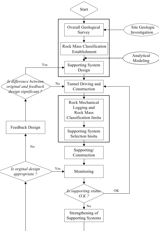
RMR and Q systems); they draw upon their experience to rate rock conditions on excavation faces; the rock conditions will dictate the support system, excavation method and construction processes, which are then specified. A typical NATM design and construction flow is illustrated in Fig. 2.1.

It must be noted that the survey and design phase is ill-equipped to predict the geologic variations underground. So while undertaking an NATM task, engineers continuously monitor and compare the geological prospecting and survey with the actual geology being excavated. If discrepancies are found, diagnostic observations are made of the actual excavated tunnel faces and appropriate modifications are adopted if necessary.

Overall Geological Survey

Start

Site Geologic Investigation

Rock Mass Classification Establishment

Supporting System Design

Tunnel Driving and Construction

Rock Mechanical Logging and

Rock Mass Classification Insitu

Supporting System Selection Insitu

Supporting/

Construction

Is supporting status O.K ? Monitoring

Strengthening of Supporting Systems Is orginal design

appropriate ? Is difference between original and feedback design significant ?

OK

No Yes

No

Feedback Design

Yes

No

Analytical Modeling

Fig. 2.1 Classical flow of NATM construction.

2.2 Geologic Exploring Method for Tunnel

Because the age of the geology in Taiwan is young, and lies between the borders of the Eurasian and Pacific plates, the land is continuously being squeezed. Due to the island’s complex geologic structures such as faults, fracture zones, joints, and soft rock, all in conjunction with abundant groundwater, tunnel disasters were once commonplace:

roofs collapsed, water flowed in, rocks burst, and squeezing occurred (Shih, 1997). It is therefore evident that the collection of accurate geological information is imperative. The exploring and recording methods for tunnel geology during the design development stage and construction stage are explained below.

(1) Design Development Stage

In this stage, geologic exploring is completed by collecting relevant documentation, and then using remote sensing and air-photo interpretation. Additionally, real investigation of the earth’s surface is required in order to understand the regional geology.

Subsequently, geophysical exploring techniques are employed, including seismic refraction, seismic reflection, downhole/crosshole velocity logging, electrical resistivity, ground penetrating radar (GPR), etc. After bore samples are taken, the analysis of the geological conditions of a construction site informs engineers as they determine the best tunnel path and select the best-fitted construction methods and tools.

(2) Excavation Construction Stage

In Taiwan, most rock tunnels are constructed using NATM. In order to determine the support method for a tunnel, every section usually will be geologically mapped and evaluated prior to excavation. After the evaluation, the 2D geotechnical map and the monitored results of the tunnel excavation face are analyzed with respect to the chosen

support system, to confirm the suitability of the tunnel support.

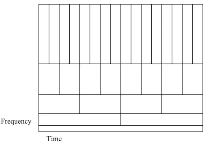
The “2D geotechnical map” shows every section and wall for every digging step in the tunnel. Using the tunnel axis as the standard length, this view stretches out the two sidewalls from bottom to top (as shown in Fig. 2.2) in the same plane as the starting point of the arch-line (Shih 1997). The 2D geotechnical map can be used not only to review the cause of disasters – should any occur – such as a roof collapse or water inflow during tunnel construction, but it can also serve as the basis of design alterations, helping engineers to evaluate geological conditions at the front before further construction.

Fig. 2.2 “2D geotechnical map” diagram

2.3 Application of Digital Image Processing

The rapid development of digital technology has increased the quality of imaging while also improving automated analysis and recognition capabilities. The image processing technology currently available includes image correction and restoration, noise restraint and analysis, image transmission technology, pattern recognition, etc., the scope of which has been applied to research in fields as diverse as physics, biology, medicine, space science, meteorology, and so on. Image technology is also broadly utilized in our daily life. Some examples are further explained as follow:

(1) Remote Sensing Image: The images obtained by air-photo remote sensing or satellite remote sensing must be treated by image processing technology, such as image restoration, noise elimination, image correction, image enhancement, image analysis, image description or classification and so on, so as to extract the usable information. At present, the main applications focus on exploration of terrain and geology in civil engineering; prospecting of resources for mining, oceanography, forestry and agriculture;

object identification for military purposes; and processing weather satellite images.

(Marceau et al. 1990; Zhang & Scofield 1994; Chen 1998; Li 1997; Jung 2000; Chen 2003; Shiu 2003).

(2) Traffic Engineering: Technology now accomplishes image processing, division, identification, and quantization of an automatically detected image, revealing damage on a road’s surface, identifying vehicle types and classifying them for traffic information, detecting accidents, searching for lost vehicles, recording license plate numbers at toll stations, and so on. (Acosta et al. 1990; Liao 1994; Chow 1995; Lee 2000; Wang 2004;

Yang 2005)

(3) Industrial and Commercial Applications: Nowadays image processing technology has been widely adopted in the quality control stage of industrial production. For example, image processing could detect surface defects on a copper plate, automatically inspect and test a system of products, and so on. Commercially the technology has even been used to fit clothing and demonstrate hair-styling. (Xlan et al. 1990; Sun & Tsai 1992;

Wen 2003)

(4) Communication Application: Video telephones and real-time video conferencing, which use Internet networks and image processing technology to complete image transmission and enhance image quality. (Lee 2000; Wang 2000; Liu 2003)

(5) Security Systems: Image technology instantly identifies fingerprints, allowing people, for example, to use their unique fingerprint instead of a duplicable key. (Yang 2000; Tsai 2000; Ho 2003; Li 2004)

(6) Medical Engineering: Physicians employ image processing to assist with diagnoses as they consult X-rays, ultrasonic images, or infrared-ray imaging. Pathological changes of tissues and organs can be viewed more accurately through image synthesis, analysis, identification, 3-D reconstruction, and so on. The computerization of medical images is divided into different parts, such as: the intake of various medical images and their output format integration, database management of cases, images and sounds, the medical image storage and transmission system, the establishment of an integrated medicine network, the processing and analysis of various medical images, expert systems for diagnosis-assistance, and user interface tools. (Yang 1994; Chang 1998; Verma & Zakos 2001; Hsu 2002; Tzeng 2004)

In the recent years, image processing technology has also been applied in the field of civil engineering. Considerable efforts have also been made in automatic recognition

of pavement images (Cherng and Miyojim 1996; Chua and Xu 1994; Guralnick and Suen 1993; Treash and Amaratunga 2000) and remote sensing images (Islam and Sado 2002; Witter et. al. 2001; Wu et. al. 2001; Liu et. al. 2000). Some efforts have been put into the automated detection of surface defects into water and sewer pipes (Moselhi and Shehab-Eldeen 1999).

As for the application of the tunnel construction, at present, the general approach is to capture tunnel images using digital cameras and then to use other approach mechanism to further analyze and recognize the tunnel-related characteristics from these images. A briefly review the application of image processing for tunnel engineering as shown in Table 2.1 (The detailed description refer to (Jiang 2000)).

Table 2.1 Applications of image processing for tunnel engineering

Method Application explanation Suitable

moment

Image Matching

To utilize the image dpi technology, that is the unit image contrasting method, in cooperation with the suitable geological structure to illustrate, then to fabricate the geological image into a geologic profile.

Construction stage

Tunnel image Scanning

To utilize tunnel image scanning system to photo the tunnel excavation face, and through naked eyes to directly observe the geological condition. In addition, it can also used to record the position on the rock bolt and its quantity etc.

Construction stage

Digital geological map

To make the image from the geological survey data of the design stage, applying the digital geological map and 3D geographical model.

However, this system is primary used on drawing and making the topographic map of large-range.

Design stage

2.4 Summary

Using various image processing technologies, we can obtain record and analyze not only the images visible to the naked eye, but also invisible data. In the past decade some researchers have endeavored to improve tunnel engineering operations in order to shorten the duration of tunnel excavation, improve the accuracy of geological evaluation, and reduce the amount of paperwork. The ultimate aim would be an automated geological record. However, the application of image processing to tunnel engineering still remains immature. In most cases where it is employed now, digital images are used merely to record and store the tunnel excavation face image. Follow-up processing and analysis have not yet been achieved.

It is hoped that the discussion and application of this research will pave the way to more efficient digital image processing technology. The basic theory and application of digital image processing will be introduced in detail in the following chapter.

CHAPTER 3

COMMON WEAK PLANES IN TUNNEL GEOLOGY

Due to geological action, the natural rock will possess many types of geological structures. Rocks––sedimentary, igneous, or metamorphic––deformed under various stress environments progressively result in a variety of flexural or fractural features (Lin 2002). These features are generally referred to as geological structure. During the deformation processes, the rock strength and the crystal environment conditions such as temperature and pressure affect the final result. The common geological structures such as bedding planes, faults, joints, and folds are referred to as discontinuous planes or weak planes in the field of engineering.

The existence of these weak planes may lead to little or no tensile strength, great distortion, high permeability, and rapid weathering during tunnel construction.

Consequently, many cave-ins in tunnel and construction accidents can occur. Weak planes may be categorized into two major types on the basis of their cause (Hung 1990;

Lin 2002):

(1) Primary Weak Planes

These are interfaces that are formed during the sedimentation process, including bedding planes and surfaces of unconformity.

(2) Secondary Weak Planes

These are weak planes that are formed by the effects of tectonic stress and the changes in the environment after the formation of rocks. It includes joints, cleavages, faults, and shear zones.

In tunnel engineering, critical weak planes such as bedding planes, joints, faults, shear zones, and folds are encountered. These are discussed in the following sections.

3.1 Bedding Planes

During the sedimentation process of a rock mass, interfaces are formed due to the differences in rock properties or similar properties but different particle sizes (fine or coarse). For example, after the sedimentation process has been in progress for a certain period of time, some coarse sands become fine mud. As a result, the coarse sands form sandstone, while the fine mud forms mudstone or shale; subsequently, a significant interface will be formed between the sandstone and shale. This is called the bedding plane. In addition, we can often observe alternating sedimentation of the sandstone and the mudstone in the hills zone; such a formation is also known as the alternation of sandstone and shale, refer to the bedding-plane diagram in Fig. 3.1(a). In addition, a natural interface may be formed due to changes in the environment of the sedimentation or volcanic activities within different phases, etc. (Hung 1990; Shih 1997)

(a) (b)

Fig. 3.1 Bedding plane diagram (a) bedding planes formed by the sedimentation of different materials (b) cross-bedding. (Shih 1997)

Sandstone Bedding Plane

Shale Limestone

The directions of most bedding planes are horizontal under undisturbed environments. Sometimes, the direction of a bedding plane can become oblique due to changes in the velocity and direction of the flows during sedimentation or later deformation under tectonic stress, etc. Further, in some thicker sandstone geologies, cross-bedding can often be found, which can be defined as a single layer or a single sedimentation unit consisting of internal laminae (very thin bed) inclined to the principal surface of sedimentation (Lin 2002), as shown in Fig. 3.1(b).

In general, a thicker rock mass usually contains many parallel bedding planes.

Because of the existence of these bedding planes, the rock strata are unable to maintain close contacts, which results in bedding plane gaps. Along the bedding plane, displacement and weathering may occur or the bedding plane gaps may be filled with soft infillings; thus, the weakness and deformability of bedding may have an adverse effect on the stability of the rock mass.

3.2 Joint

Regular shear fractures that can be observed inside rocks are called “joints.” They are fractural surfaces that are caused by the deformation due to tectonic stresses or other geological effects. In general, they are also known as “fractures” and are considered as gaps inside rocks, that is, the rocks on either side of such a gap do not show a relative displacement along the direction of the gap.

A joint surface is normally planar; however, curved surfaces also occur. Joints intersect rock mass in various attitudes and extend to various scales. Furthermore, a joint is usually part of a group, but rarely, they can form singly. Joints that are formed as a set and are parallel to each other are called joint sets. The spacing between

adjacent joints in a joint set can range from several centimeters to several meters (Lin 2002). On occasion, more than two joint sets may be formed in a single rock mass, as shown in Fig. 3.2

Once a joint has occurred, the shear strength at the joint surface will generally be lower than that of the intact rock mass. Most joints are unclosed gaps; thus, in addition to high permeability, weathering occurs easily and causes discoloration, softening, fracture, or even mixing with mud.

Fig. 3.2 There are two joint sets (layers 7 and 8) in the rock mass (Hung 1990).

3.3 Fault and Shear Zone

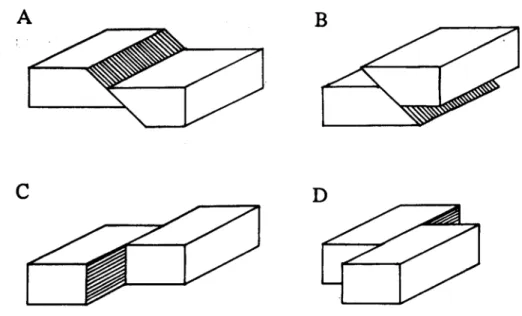
A fault is regarded as fracture deformation. When a rock is subjected to a massive tectonic stress, relative displacements occur across fracture surfaces, such as the up-down, left-right, and forward-backward movements. Such fracture surfaces are called fault planes, and they may have clear sharp fracture surfaces. However, these fracture surfaces are mostly fractured zones with variable thicknesses. Hence, such zones are called fault zones. Fault zones normally consist of fragments and breccias of rocks from both sides of the fault, and sometimes they may contain several sub-faults in the interior. In addition, the fault plane can intersect the rock mass at a variety of angles.

Fig. 3.3(a) and (b) are sketches of a fault plane and fault zone, respectively. On the basis of the above mentioned characteristics, faults can be categorized into three major types: (Hung 1990; Shih 1997; Lin 2002)

(a) (b) (c)

Fig. 3.3 (a) Fault plane, (b) fault zone, and (c) shear zone diagram (Wu 1982).

(1) Normal Faults: If the hanging wall has moved downward relative to the footwall, the fault is called a normal fault; this is formed due to the horizontal extension or the vertical uplift of the crust. Because the direction of the main stress is identical to that of the earth’s gravity, such faults are called gravity faults. In addition, the dips of such faults are usually at high angles, between 65° and 90°, as shown in Fig. 3.4 (a).

(2) Reverse Faults: If the hanging wall has moved upward relative to the footwall, the fault is called a reverse fault; this is formed due to the horizontal compression and contraction of the crust. In addition, the dips of such faults are smaller (under 45°), and sometimes the fault plane can be almost horizontal, as shown in Fig. 3.4 (b).

(3) Strike-Slip Faults: If a vertical fault plane has movements only in the horizontal plane, the fault is called a strike-slip fault; this is also formed due to the horizontal

compression of the crust. Further, they can be categorized into left-lateral faults and right-lateral faults, as shown in Fig. 3.4 (c) and (d).

Once a fault has occurred, it usually causes the rock to be considerably more fractured, and this further increases the weathering activity. If the slip of the fault continues, the fractured rocks are crushed and become fault breccia with specific thicknesses. Alternatively, they may be ground further and become fault gouges. As a result, the strength of the rock mass is decreased and its permeability is increased. This compromises the stability of the rock mass.

A shear zone (Hung 1990; Yang 1994) may have several sets of slip planes or shear planes that intersect over a certain area. However, some scholars (Wu 1982) believe that shear zones are zones where rocks slips intersect each other similar to the case of a fault; however, such apparent and significant developments do not occur, as shown in Fig.

3.3(c).

Fig. 3.4 Based on the direction of movement of the hanging wall and footwall, a fault can be classified as (a) normal fault, (b) reverse fault, (c) left-lateral fault, and (d) right-lateral fault. (Yang 1994)

3.4 Fold

Under tectonic stress squeezing, rocks deform and buckle in a wavy pattern. This phenomenon is called a “fold.” The amplitudes and shapes of folds depend both on rock properties such as thickness and strength and on the conditions of the deformation environment, such as temperature and pressure. The amplitudes of folds range from several centimeters to several kilometers, and their shapes vary greatly from elongated and circular to even some irregular shapes.

Based on the structure, folds can be divided into two categories: anticline and syncline, as shown in Fig 3.5. An anticline fold has a convex-upward form with older rocks in the central core. The bedding of both limbs dips away from the core. In contrast, a syncline fold has a concave-upward form with younger rocks in the central

if the angles of the two limbs of a fold are similar and the fold has a perpendicular axial plane, it is called a “symmetric fold.” On the contrary, if the angles of the two limbs of the fold are different, it is called an “asymmetric fold.”

(a) (b)

Fig. 3.5 (a) Anticline and (b) Syncline. The directions of the arrows represent the direction of younger rock strata. (Yang 1994)

Once a fold has occurred, it is an irreversible structural change that also can cause other phenomenon in the rock; for example, since the slipping phenomenon occurs in between the layers, the limbs or hinge of the fold may crack and geological structures such as cleavages or joints are formed. Therefore, the rock becomes more fragile and the rock mass slides down easily, thus, leading to the easy infiltration of groundwater.

CHAPTER 4

DIGITAL IMAGE PROCESSING

In this chapter, an overview of the image processing is introduced. First, we introduce the basic concept of the digital image in Section 4.1. Next, we introduce image processing in the spatial and frequency domains in Section 4.2 and Section 4.3 respectively. In Section 4.4, we further introduce the basic theory of wavelet transform.

Finally, in Section 4.5, we briefly review the basic concepts of image recognition.

4.1 Introduction

Images are two-dimensional representations of the visual word. The image which humans see with the naked eye is called an analog image. But a computer cannot receive analog data; it can only receive digital. Briefly, an analog image becomes digitized in space and values after being sampled and quantified. It then forms a digital array (usually, equal interval sampling and quantification are adopted). A digital image can be regarded as a 2D array. Each smallest element in an array is called a pixel. The value of a pixel is called “gray level” which is indicated by integers from 0 ~ 255 as shown in Fig. 4.1.

After digitizing an image, a powerful computer can help us to process and analyze the information shown in such an image to improve the image quality and enhance a human’s understanding of the image and a computer’s recognition of the image. Image processing has already found applications in the fields of physics, biology, medical science, space science, and meteorology, as well as in daily life where it accomplishes word recognition, fingerprint identification, remote sensing images and medical images (see Section 2.3).

Fig. 4.1 A 2D digital image diagram

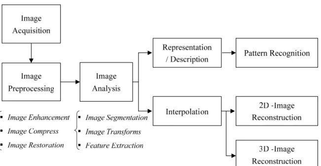
However, image processing is not a one-step process. We are able to differentiate several steps which must be performed one after the other until we can extract the data of interest from an observed image (Gonzalez & Woods 1987). Common image processing operations are shown in Fig. 4.2. First, the digital images are obtained by a camera. Then, selecting a suitable procedure depends on the aim of image processing application. For example, image recognition (or object inspection) can be applied to identify (or inspect) the objects of interest. In general, this is a complex procedure requiring a variety of steps that successively transform the iconic data to recognition information. So the image recognition process requires the use of tools such as image enhancement, image segmentation, feature extraction, pattern recognition, and so on. The details relating to image processing technologies at different phases are introduced in the following sections.

Fig. 4.2 Common image processing operations

4.2 Image Processing in the Spatial Domain

Image enhancement and image segmentation are often referred to as image preprocessing. Preprocessing is used to perform initial processing that makes the primary data reduction and analysis easier (Green 1983). Image preprocessing can be performed in the spatial and frequency domains, but here we discuss image preprocessing only in the spatial domain.

4.2.1 Image Enhancement

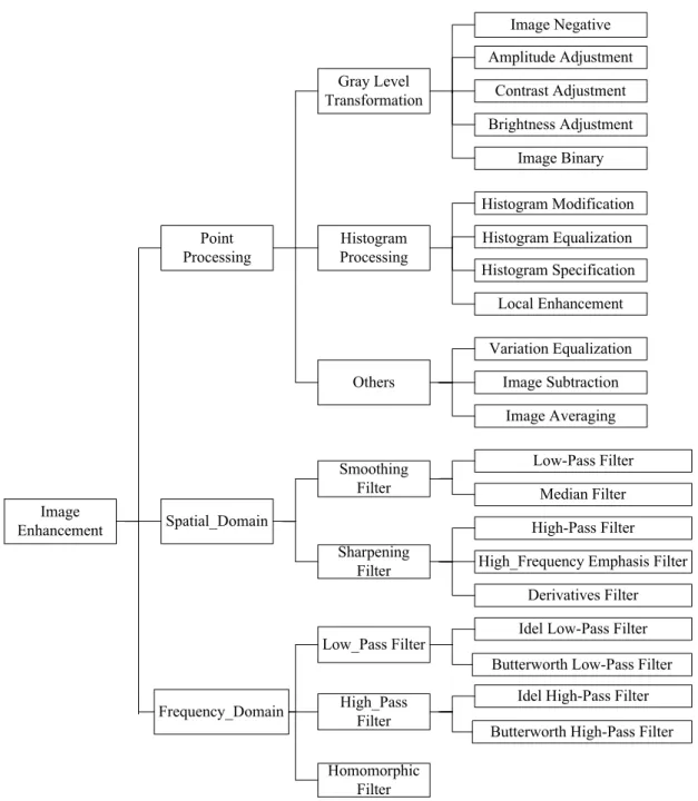
The purpose of image enhancement is to filter out noise and strengthen salient image features, and it is especially useful when dealing with complicated images. There are three types of image enhancement: point enhancement, spatial domain enhancement and frequency domain enhancement (shown in Fig. 4.3) (Gonzalez & Woods 1987; Jain 1989; Pratt 1991).

Image Enhancement

Frequency_Domain Point Processing

Spatial_Domain

Image Negative

Image Binary Gray Level

Transformation

Low_Pass Filter

Image Averaging Image Subtraction Histogram Equalization Histogram Modification Histogram

Processing

High_Pass Filter

Butterworth High-Pass Filter Idel High-Pass Filter Butterworth Low-Pass Filter

Idel Low-Pass Filter Contrast Adjustment Amplitude Adjustment

Brightness Adjustment

Histogram Specification Local Enhancement

Others

Variation Equalization

Sharpening Filter Smoothing

Filter

Low-Pass Filter

Derivatives Filter High_Frequency Emphasis Filter

High-Pass Filter Median Filter

Homomorphic Filter

Fig. 4.3 Image enhancement methods.

Point enhancement is an image enhancing technique that directly revises the gray levels of individual pixels, without considering the effect on surrounding pixels. Basic point image enhancement methods perform addition and subtraction on the gray level value of each pixel or eliminate some specific mingled noises. Typical point image enhancement procedures include image negation, amplitude adjustment, contrast adjustment, and brightness adjustment, among others (Green 1983; Jain 1989; Pratt

1991). Generally, point image enhancement is less helpful in characteristic identification and extraction for images of nature.

Spatial-domain-based image enhancement adopts specific masks (e.g., 3x3, also referred to as templates, windows, or filters), which perform the image enhancement processing (Gonzalez & Woods 1987; Jain 1989; Pratt 1991). A mask is a small 2D array as shown in Fig. 4.4, where w1, w2 …w9 represent mask coefficients. The mask allows various operations over some neighborhood of specific pixels. Generally, it uses a square or rectangular sub-image area centered at a specific pixel. The center of the sub-image moves from pixel to pixel. For example, the center of the 3x3 mask is moved around the image as shown in Fig. 4.5. At each pixel position in the image, we multiply every pixel that is contained within the mask area by the corresponding mask coefficient. The formula can be defined as follows:

[

]

( ) ( ) ( )

( 1, 1) ( , 1) ( 1, 1) (4.1) ,

1 ,

1 , 1

1 , 1 1

, 1

, 1 ,

9 8

7

6 5

4

3 2

1

+ + +

+ +

+

− +

+ +

+

−

− +

− + +

− +

−

−

=

y x f w y

x f w y

x f w

y x f w y x f w y

x f w

y x f w y

x f w y

x f w y x f R

Therefore, the grey level at the center point (x, y) of a mask can be substituted by R, until all pixels are substituted.

W1 W2 W3

W₄ W₅ W₆ W7 W8 W9

Fig. 4.4 The 3x3 mask and the corresponding position representation

Fig. 4.5 The operation of the 3x3 mask

Spatial-domain-based image enhancement techniques are usually divided into two categories: smoothing filters and sharpening filters. Smoothing operations are used primarily to diminish spurious effects that may be present in a digital image and to reduce noise in an image. They are frequently composed of low-pass filters, median filters and high-pass filters and each concentrates on a specific energy frequency domain.

For example, low-pass filters emphasize the energy of a typical image concentrated primarily in low-frequency components. Using smoothing filters, some noises in a complex image may be removed and significant image characteristics may be more easily identified. In contrast, sharpening filters are useful primarily as enhancement tools for highlighting edges in a digital image. The edges and details of image characteristics can be more readily seen through sharpening filters. Median-pass and high-pass filters have stronger ability to sharpen edges in digital images, but they may also eliminate features or pixels required for reservation due to their comparatively aggressive

computing algorithms. Different spatial-domain-based image enhancement methods are useful in different places at different times. The selection of spatial-domain-based image enhancement techniques is subjective and experience-oriented. In some cases, superior results may be obtained using a combination of different filters.

4.2.2 Image Segmentation

The main goal of the image processing is to extract meaningful features from a digital image. Image segmentation serves this purpose. Image segmentation extracts constituent parts or objects from the background (Gonzalez & Woods 1987), and it is an important step in image analysis where objects or other entities of interest are extracted from an image for subsequent processing, such as description and recognition (Minor &

Sklansky 1981). Image segmentation algorithms are generally based on one of two basic properties of gray-level values: discontinuity and similarity. The former is based on the mutation segmentation of gray-level, which is primarily applied to the inspection of isolated image points and segment edges. The principal approaches of the latter are based upon thresholding to perform the regional growing, regional splitting and merging.

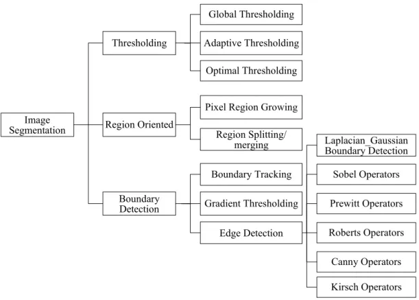
Popular image segmentation approaches are shown in Fig. 4.6.

Image Segmentation

Boundary Detection Thresholding

Region Oriented

Adaptive Thresholding

Boundary Tracking Gradient Thresholding

Optimal Thresholding

Region Splitting/

merging Pixel Region Growing

Edge Detection

Sobel Operators

Canny Operators Roberts Operators

Prewitt Operators Laplacian_Gaussian Boundary Detection

Kirsch Operators Global Thresholding

Fig. 4.6 Image segmentation methods.

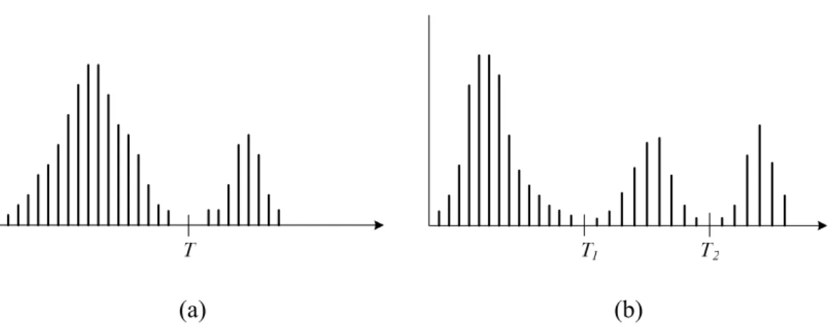
Thresholding is one of the most important approaches to image segmentation. To illustrate the basic concept of thresholding, let us suppose a gray level histogram as shown in Fig. 4.7. The histogram corresponds to an image, f(x, y), composed of light objects on a dark background, such that object and background pixels have gray levels grouped into two modes. One can select a threshold T that separates objects from background. A threshold image f(x, y) can be expressed as follows:

( ) (4.2)

) , ( 0

) , ( , 1

⎭⎬

⎫

⎩⎨

⎧

≤

= >

T y x if

T y x y if

x f

Pixels labeled 1 correspond to objects while pixels labeled 0 correspond to the background. As a matter of fact, the method is binary. Good results can be achieved when there are simple objects against a background with clear contrast.

Threshold-based segmentation adopts various thresholds to recognize interesting objects from images. When T depends only on the image f(x, y), the threshold is called a global threshold. If T depends on an image f(x, y) and a coordinate p(x, y), the threshold is termed a local threshold. Additionally, if T depends on the spatial coordinates x and y, it is called a dynamic threshold. But often an image may not be as simple as the one described above. There may be various changes in the background, for instance. Under such circumstances, the threshold values used in certain regions may not be applied to other regions. Consequently, adaptive and optimal thresholds are also proposed (Miao 1999). In conclusion, threshold-based segmentation method is most applicable to segmentation problems with clear and close boundaries between interesting objects and backgrounds.

(a) (b)

Fig. 4.7 Gray-level histograms that can be partitioned by (a) a single threshold, and (b) multiple thresholds.

Region-oriented segmentation partitions an image into several sub-regions Ri. pixels within a sub-region have certain characteristics; for example, the grey values are within the same range. This is defined as follows (Miao 1999):

(1)

U

(2) Ri is a connected region, i = 1, 2, . . . , n (3)^Ri

I

(4)P( )R_i =TRUE for i = 1,2, . . . , n (5)^P

(

U

)

WhereP( )R_i is a logical predicate defined over the points in set Ri, and φ is the null set. However, methods like region growing by pixel aggregation and region splitting and merging are based on the region-oriented segmentation which we do not elaborate here. Please refer to related literature if interested (Gonzalez & Woods 1987; Jain 1989).

There are many ways of dealing with boundary detection-based segmentation. The first-order or second-order derivatives are mainly used for boundary detection. For example, edges are detected based on the first-order derivative. Then smaller edges are connected to a boundary by applying the directions of the first-order derivative. Most boundary detection adopts the aforementioned method. As to the first-order and second-order derivatives for image f(x, y), we define them as follows:

( ), ( ), f( )x,y j (4.3) i y

y x x f y x

f ∂

+ ∂

∂

= ∂

∇

( ), ( ), ₂ ( ), (4.4)

2 2

2 2 f x y j

i y y x x f y x

f ∂

+ ∂

∂

= ∂

∇

where ∇f( )x,y represents the maximum rate of increase of f(x, y) per unit distance in the direction of the gradient vector. The purpose of finding the degree of a gradient is to locate the grey value with the maximum change in an image. Usually this occurs at the boundaries of objects.

Edge detection is by far the most common approach for detecting meaningful discontinuities in gray level. An edge appears in the boundary between two regions with relatively distinct gray-level properties. The idea underlying most edge detection techniques is the computation of a local derivative operator. It mainly adopts first and second derivatives to determine object boundaries. The magnitude of the first derivative can be used to detect the presence of edges. The sign of the second derivative can be used to determine the location of edge pixels. A great deal literature is concerned with boundary detection. The Sobel operation and Laplacian of Gaussian are among the more famous (Gonzalez & Woods 1987). In this study we will confine ourselves to discussion only of the Sobel operation.

Sobel edge detection employs a high-pass filter designed to remove smooth parts in images. The remaining parts represent the pixels where gray levels are changing rapidly, that is, at pixels that lie on edges. The Sobel algorithm is based on the same concept as gradients; the gradient of an image f(x, y) at location (x, y) is defined as the following:

( ) ( , ) ^{2 2} (4.5)

2 2

y

x G

y G f x

y f x f f

magnitude ⎟⎟ = +

⎠

⎜⎜ ⎞

⎝

⎛

∂ + ∂

⎟⎠

⎜ ⎞

⎝

⎛

∂

= ∂

∇

=

∇

For a discrete digital image, the above formula can be rewritten as follows:

( ) ( )

( ² ) ( ² ) ^(4.7)

) 6 . 4 ( 2

2

7 4 1 9 6 3

3 2 1 9 8 7

p p p p p p G

p p p p p p G

y x

+ +

− + +

=

+ +

− + +

=

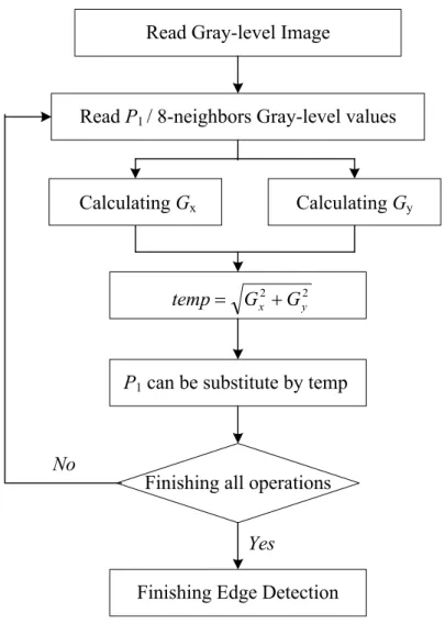
where Gx andGy represent the components of the gradient vector in the x direction and in the y direction. A 3x3 mask as shown in Fig 4.8(a), P5 represents the gray level at location(x, y) and the other Pi represents the gray level of the 8-neighbors of (x, y). The difference between the third and the first rows of the adjacent regions to a 3x3 mask is similar to the derivative in the x direction as shown in Fig 4.8(b) while the difference between the third and first columns shown in Fig 4.8(c) is similar to the derivative in the y direction. Regarding the spatial algorithm, only multiplication and addition of grey values of pixels can be calculated due to the adoption of the mask. The above calculation is efficient. However, the Sobel edge detection is unsuitable for image detection at a tunneling site based on our review of relevant literature (Jiang 2000; Wu 2000). The processing flow relating to Sobel edge detection is shown in Fig 4.9.

P1 P2 P3

P₄ P₅ P₆ P7 P8 P9

-1 -2 -1

0 0 0

1 2 1

-1 0 1

-2 0 2

-1 0 1

(a) (b) (c)

Fig. 4.8 Sobel operation diagram:(a) a 3x3 mask (b) the x direction(c) the y direction.

Read Gray-level Image

Read P1 / 8-neighbors Gray-level values

Calculating Gx Calculating Gy

2 2

y

x G

G temp= +

P₁can be substitute by temp

Finishing all operations

Finishing Edge Detection Yes

No

Fig. 4.9 The processing flow as it relates to Sobel edge detection.

4.3 Image Processing in the Frequency Domain

In recent decades, transformation theories have played an important role in signal processing and image processing. Images are viewed conceptually as a type of signal.

By converting images into frequency domains through various signal transformation methods, image features can be analyzed from another point of view. An image can be converted to stationary signals, based upon Z transform, Laplace transform, Fourier transform, and so on (Burrus et al 1988; Hubbard 1994; Rao & Bopardikar 1998). Of

those, the Fourier transform is the most broadly applied. The Fourier transform pair can be defined by the equations (4.8) and (4.9):

( ) f( )xe dx (4.8) f ω ^{∞ −iωx}

∞

−

∧ ⁼

∫

( ) ^{( ) (4.9)}

2

1 ω ω

π

ω d e f x

f

∫

= ∧

Equation (4.8) represents the Fourier transform of f(x) and equation (4.9) represents the inverse Fourier transform.

In general, there is huge quantity of data in an image. To enhance the efficiency of calculations, a Fast Fourier Transform (FFT) has been proposed (Gonzalez & Woods 1987). Its advantage lies in reducing calculations and employing simple operations with a calculator. Many real-world applications such as radar, sonar, image processing, etc.

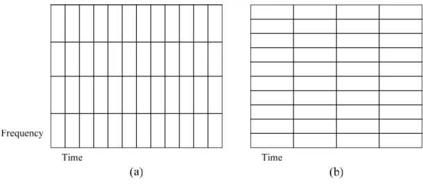
adopt spectrum calculations. Signals which are time-varying are categorized as non-stationary signals. The spectrum converted from signals by the Fourier transform is unable to completely present the actual variables of signals. That is to say, the so-called “irregularity”, of signal f (x, y) in the spatial domain is suddenly regarded as high-frequency signal. The changes in frequency through the conversion of the Fourier transform are distributed on the overall frequency axis. Therefore, the positions of spatial domain become very important (Gonzalez & Woods 1987; Froese 1996).

To deal with time-varying, non-stationary signals, several signal processing techniques have been established in the past decade. First, Gabor (Gabor 1946; Graps 1995) pointed out the concept of windowed Fourier transform (WFT) which is augmented with a window function g(x). The function is also call Short-Time Fourier Transform (STFT) defined in the following formula (4.10):