複合加減法3D列印流程對於多異種的物件製作

(1)

國立臺灣大學電機資訊學院電機工程學研究所碩士論文

Department of Electrical Engineering

College of Electrical Engineering and Computer Science National Taiwan University

Master Thesis

複合加減法 3D 列印流程對於多異種的物件製作

Hybrid Additive and Subtractive 3D Printing Process for Multi-Heterogeneous Objects Fabrication

曾柏凱 Po Kai Tseng

指導教授：羅仁權博士 Advisor: Ren C. Luo, Ph.D.

中華民國 106 年 7 月 July 2017

(2)

誌謝

碩士班這兩年是人生中的另一個階段，在這階段中自我充實而且留下一段美好的回憶。兩年的碩士生涯中說長不長說短不短，但是轉眼間來到鳳凰花開的季節，

意味我們又將即將往下一個階段邁進。回想起剛來到一個陌生的台大校園，接觸陌生的人事物，一開始還有點憂心與擔心，但進入一個有熱心的學長姊、親切的同學與學弟妹的實驗室，很快就融入生活中。感謝父母，在我面臨低潮時給於我鼓勵與支持，感謝口試委員，張帆人老師以及顏炳郎老師百忙之中特地抽空給予我的論文諸多的建議及指教，感謝指導教授羅仁權教授，不僅提供們豐富的研究資源外，在學術知識上教導我們向深度與廣度發展，在實務方面培養我們動手做的能力，此外，

老師還給予我們非常多的國際觀世界觀，並教誨我們待人處事的道理與社會上應對的準則，讓我獲益良多。最後，還要感謝鐿文與東榕學長，與學長討論研究方法和技術瓶頸問題，並一一克服眼前的困難，並且在不斷的摸索中漸漸了解自己的研究興趣，並在未來會繼續朝向此方面更加努力。

在國立台灣大學智慧機器人及自動化國際研究中心 (NTU-iCeiRA) 的兩年研究生活中，我要感謝鐿文、瑋隆、献章、陞祐、繼棠、金成、玲盈、昕昳、東榕、

旭佳、禮聰、志遠以及正倫等博班學長姊，還有柏任、士紘、智賢等碩班學長姊，

以及同屆共同奮鬥的夥伴達方、俊豪、長鈞、晴岡、李晟、孟勳、靖霖、昱佑、仲凱、莉彤、凱鈞、立揚，最後還有積極認真的學弟妹錦賢、名彥、育榕、石崴、育澤、智堅、武昱、威辰、展嘉、王昊、培淳、嵩詠、何鑫以及曾旻，以及助理雯雅 (Tracy)、煜倫(Dornin)。感謝大家的支持與幫助，不分晝夜地討論研究，同甘共苦地參加比賽熬夜為比賽而努力，在研究之餘還會一起運動一起玩樂，非常開心這段日子能和大家一起奮鬥與生活點滴，你們都是我一生難忘的回憶。

能完成這篇論文，我要感謝在我生命中出現的每一個人，真的能遇見你們真好，

非常謝謝你們。

曾柏凱謹誌一百零六年七月

(3)

中文摘要

近年來 3D 列印技術越來越流行，並且運用於各種產業，如航太業、工業甚至醫學工程方面，其主要優點為客製化及快速製作，以達到縮短產品週期並提高產品設計之自由度。但是隨著產品的多樣性與複雜性，單純的加工以無法獨力製作完成，

因此我們設計出複合加工機(加法及減法)，用以完成多樣且複雜的產品。並且產品可能是由多個零件或多個物件所構成的，但目前所使用的 3D 列印都是多個物件同一層先印完再移動至下一層，噴頭會在物件間頻繁移動，不但消耗能源而且拖累完成的時間，因此，在此論文中，我們將提出加法製作多物件流程優化之演算法以及減法路徑規劃完成客製化雕刻。

首先，在加法製作流程優化分為三大步驟，1.針對每個物件作放置之最佳化，

以減少列印時所產生支架達到節省材料與去除支架的程序，2.多物件進行集裝優化 (bin packing)規劃物件擺放位置，並且結合最短路徑演算法(travelling salesman problem)，有利於噴嘴移動過程中，可以使噴嘴有效率之移動，3.加法路徑優化配合硬體上的最大限制，使得列印更加有效率，對比常見方法在演算法中大量減少在物件間移動的頻率，不僅可以節省製作時間外，還可以節約能源。在加減法製作流程，當列印加工完成後並將物件資訊轉換至減法坐標系，並將物件所要雕刻區域利用保角映射(conform mapping)作攤平展開得到二維平面，並使用彈簧質量模型 (spring mass model)基於三角形邊長做優化以減小攤平曲面之誤差，接下來二維圖形投影至攤平的二維平面上，再將平面轉換至物件表面，以取得減法路徑軌跡，以完成加減復合之工程，並實現在我們實驗自行開發的龍門式複合加工機上。

關鍵字：3D 列印技術、複合加工機、集裝優化、最短路徑演算法、龍門式複合加工機

(4)

Abstract

In recent years, three dimensional (3D) printing is the fastest growing technology.

Nowadays, it has been largely applied in aerospace industry, industry and medicine engineering, etc. Additive manufacturing (AM) technologies not only reduce the new product development cycle, but also develop unique style models to satisfy users’

requirements. However, the additive manufacturing cannot complete the diversity and complexity products independently. We design the hybrid 3D printing machine including the additive and subtractive processes to complete the products. And the products may be composed of the many parts or objects. In the common slicing software, the 3D printers print an object layer by layer. However, when multiple objects are printed at the same time, the nozzle moves among objects and always increases enormous distance of the transition travel. Therefore, in this thesis, we propose a novel addition process optimization algorithm and develop the trajectory planning of the subtractive process to carve the customized logo or image.

In the beginning, the optimization of the addition process is divided into three main steps. 1. The optimization for locating each specific object is implemented to minimize the supports during the printing procedure. This step can efficiently save the materials and consume less time for remove the supports. 2. Two dimensional packing problem for planning location of multiple objects is combined with the traveling salesman problem to promote the spray efficiency of nozzle. 3. With consideration of the workspace and hardware limitation, the printing time is apparently decreased by addition path optimization. Compared with the common path planning strategy, the advantage of the proposed path planning minimizes the frequency of movement among

(5)

each object. This proposed algorithm effectively decreases time consuming on printing and saves energy consuming furthermore. For subtractive process, the object information can be obtained from additive process and is transformed to subtractive coordinate system. The sculpture region of the 3D object is initially expanded into 2D space by conform mapping, and the vertices of the flattening plane are adjusted to appropriate positions using spring mass model with edge-based flattening algorithm to minimize distortion of flattening plane. Then the 2D image can be intuitively projected onto the expanded plane by geometrical transformation. The projected product in 2D space can be reversely transformed into 3D space, where the reconstructed surface is fitted onto the original surface of the object. Therefore, the subtractive part can run along the path that is generated by above steps. We have demonstrated the success of the proposed methods by using the development of hybrid 3D printing machine consisting of additive and subtractive processes in our NTU robotics and automation lab.

Keywords: three dimensional printing, hybrid 3D printing machine, additive manufacturing, additive and subtractive processes, two dimensional packing problem, traveling salesman problem

(6)

LIST OF FIGURES

Figure 1.4-1 The illustration of fused filament fabrication ... 8

Figure 1.4-2 Fused filament fabrication ... 8

Figure 1.4-3 Compare the difference between SLA and DLP. SLA : selective exposure to light from laser. DLP : selective exposure to light from projector. ... 9

Figure 1.4-4 The illustration of Digital light processing (DLP) ... 9

Figure 1.4-5 The printing process of running shoe ... 10

Figure 1.4-6 The illustration of selective laser sintering ... 10

Figure 1.4-7 The result of selective laser sintering ... 11

Figure 1.4-8 The result of selective laser melting ... 11

Figure 1.4-9 the illustration of laser metal deposition (LMD)... 12

Figure 1.4-10 Laser metal deposition (LMD) ... 12

Figure 2.1-1 There are two parts on the gantry-type hybrid machine. Left side is the additive (3D printing) part while right side is subtractive (cutting) part. ... 15

Figure 2.1-2 Definition of the D-H parameters ... 17

Figure 2.1-3 Control architecture ... 18

Figure 2.1-4 UTC controller ... 19

Figure 2.1-5 Arduino MEGA 2560 ... 21

Figure 2.1-6 stepper motor driver ... 22

Figure 2.1-7 Stepper Motor... 24

Figure 2.2-1 STL file and format ... 25

Figure 2.2-2 (a) CAD model (b) STL format (c) higher resolution STL format ... 25

Figure 2.2-3 KISSlicer slicing software [27] ... 26

Figure 2.2-4 G-Code file ... 27

Figure 2.2-5 Direct numerical control ... 29

Figure 2.3-1 PLA (Polylactic Acid) ... 30

Figure 2.3-2 ABS (Acrylonitrile Butadiene Styrene) ... 31

Figure 3.1-1 system flowchart of additive manufacturing for multiple objects ... 32

Figure 3.2-1 table posture 1 (estimated build time: 43.38 minutes) ... 34

Figure 3.2-2 table posture 2 (estimated build time: 30.95 minutes) ... 35

Figure 3.3-1 the left image is Moai model. Top right is the top view of the Moai model and lower right is the irregular contour. ... 36

Figure 3.3-2 red rectangle is original bounding rectangle (Area : 588.816 𝑐𝑚2), and green is minimum bounding rectangle (Area : 529 𝑐𝑚2) ... 37

Figure 3.3-3 The illustration about collision region definition ... 38

(10)

Figure 3.3-4 the dark gray area is maximum contour of model, and the green is minimum bounding rectangle. The red, blue and gray rectangle are corresponded to situation 1, 2

and 3 respectively. ... 39

Figure 3.4-1 the blue line represents the printing paths and the red line is transition paths. ... 40

Figure 3.5-1 the illustration of two-dimensional packing problem. ... 44

Figure 3.5-2 The illustration of the roulette wheel selection ... 45

Figure 3.5-3 Cumulative probability... 46

Figure 3.5-4 Case 1 selective crossover ... 48

Figure 3.5-5 Case 2 selective crossover ... 48

Figure 3.5-6 Case 3 crossover by using weighted average ... 48

Figure 3.6-1 Velocity and acceleration profiles. On printing path segments 𝑡1~𝑡2 , 𝑡3~𝑡4 and 𝑡7~. On transition path segments 𝑡0~𝑡1 , 𝑡2~𝑡3 and 𝑡4~𝑡7. ... 53

Figure 4.1-1 system flowchart ... 56

Figure 4.2-1 Triangle to triangle mapping ... 58

Figure 4.2-2 (a) the mesh of the 3D model. (b) the flattening surface by using conformal mapping (c) the vertices unifying procedure. ... 61

Figure 4.2-3 the edges and angles around the vertex 𝑡𝑎 ... 63

Figure 4.3-1 The illustration of the system coordinate simulation ... 68

Figure 5.1-1 The extrusion system has some components including a nozzle, a stepper motor, a heater, a thermocouple, etc. ... 71

Figure 5.1-2 The relationship of nozzle velocity and extrusion speed reflects in the quality of the results. ... 71

Figure 5.1-3 (a) tooth (b) Taipei 101 (c) pen holder (d) Moai (e) statue ... 72

Figure 5.1-4 Location of multiple objects with top view ... 73

Figure 5.1-5 Cost function (best chromosomes in genetic algorithm)... 73

Figure 5.1-9 The result by our proposed method. The blue line represents the printing path and the red line is transition path. ... 75

Figure 5.1-11 Cost function (best chromosomes in genetic algorithm) ... 76

Figure 5.1-12 Ideal result of the printing ... 76

Figure 5.2-1 The three different carving tools. Left to right : (a) The cone drill. (b) The twist drill. (c) The round drill. ... 79

Figure 5.2-2 The tool tip after subtractive process. ... 79

(11)

(b) The twist drill. (c) The round drill. ... 81 Figure 5.2-4 (a) the triangular mesh of the 3D model. (b) flattening result. (hemisphere mesh

data: number of vertex : 145; number of face : 264 ). ... 82 Figure 5.2-5 (a) the triangular mesh of the 3D model. (b) flattening result. (wave mesh data:

number of vertex : 400; number of face : 722 ) ... 82 Figure 5.2-6 The left is 2D image and the right is the planned path by greedy algorithm. The

red line is the transition path and the carving path is labeled as blue line... 84 Figure 5.2-7 Show the projected results on the geometric models. ... 85 Figure 5.2-8 The black line which 2D data is projected onto the 3D different models.

Compared with projection algorithms, the red line is our proposed algorithm and the blue line is orthogonal projection method. ... 85 Figure 5.2-9 the process of additive and subtractive manufacturing with front view and side

view ... 86 Figure 5.2-10 (a) The original STL model. (b) The projected simulation on the model. (c) The

carving result on printed model. ... 87 Reverse engineering, also known as back engineering, is the processes of extracting

knowledge or features from anything man-made and reconstructing it or reconstructing anything based on the extracted information. In the experiment, using the Skanect 3D scanning software [29] and Kinect one reconstructs the model and the printing result is shown in Figure 7.1-1. ... 89 Figure 7.1-2 Skanect 3D scanning software and printing result ... 89

(12)

LIST OF TABLES

Table 1 Compare with additive manufacturing methods ... 13

Table 2 Specifications of UTC controller ... 19

Table 3 Specifications of Arduino MEGA 2560 ... 21

Table 4 Pins introduction of driver ... 23

Table 5 Running current setting ... 23

Table 6 the setting about stop current, excitation mode and decay setting ... 23

Table 7 the basic setting in the slicing software ... 26

Table 8 the common G-Code in 3D printers ... 28

Table 9 the difference between PLA and ABS ... 31

Table 10 the production time analysis on the printing and transition paths (model information: height is 100mm, number of layers is 392) ... 41

Table 11 the building time for each object ... 72

Table 12 the production time of three strategies ... 77

Table 13 Compare with typical methods on hemisphere surface ... 82

Table 14 Compare with typical methods on wave surface ... 83

Table 15 Compare average length error (mm per unit) with orthogonal projection on projection results in Figure 5.2-8. ... 86

(13)

Chapter 1 Introduction

1.1 Introduction

In the recent years, three dimensional (3D) printing is the fastest growing technologies. Compared with traditional manufacturing techniques, 3D printing has some advantages such as ability of product customization and rapid prototyping, low cost of production, material saving, and ease of designing and manufacturing. Fused Filament Fabrication is a method of the extrusion-based 3D printing. With this method, the thermoplastic material, like Acrylonitrile Butadiene Styrene (ABS) or Poly-Lactic Acid (PLA), becomes gelatinous liquid by heater. Then the material is deposited as the filament through the extruder nozzle which moves along a manufacturing path. However, the extrusion-based 3D printer has limited in manufacturing time which depends on the complexity and size of models.

In nowadays, 3D printing is widely applied in industry, aerospace and medicine, etc.

For example, in the aerospace industry, Airbus announced that its new Airbus A350 XWB included over 1000 components manufactured by 3D printing. GE Aviation revealed that it had used design for additive manufacturing to create a helicopter engine with 16 parts instead of 900, with great potential impact on reducing the complexity of supply chains.

In the medicine, 3D printing prosthetics are also used for the treatment of injured animals.

In the construction industry, the new company, “Apis Cor” in San Francisco, has developed a cost-effective solution to build a house that can be built in less than 24 hours.

In the Automotive industry, Local Motors debuted Strati, a functioning vehicle that was entirely 3D Printed using ABS plastic and carbon fiber, except the powertrain.

(14)

1.2 Motivation and Objective

The 3D printing technology develops rapidly in the past decades. The 3D printer is based on the technology of additive manufacturing. It builds an object layer by layer so that it can fabricate a very complicated geometrical object.

On the additive process, we focus on the multi-objects printing efficiently. The two key points are mentioned that one is the locations of the multiple objects and another is the times and length of the transition travel. The printing location of the multiple objects directly influences the length of transition path, and then the manufacturing time changes with it. Therefore, planning the location of the objects is significant. On the other hand, we all know that the printer will not move to the next layer until it completes the all machine path on the current layer with traditional 3D printing method. So when the multiple models are printed, the traditional method generally takes much time on the transition travel where the nozzle moves along among the objects without printing. The transition travel is necessary for multiple models but it is so excessive that the process will become inefficient. As a result, minimizing the times and length of the transition travel as much as possible is very important.

On the subtractive process, as the industries and manufacturers having the increasing demands of customized production, such as remarking serial number and carving the logo or brand on the surface product, neither the additive nor subtractive manufacturing can satisfy all the requests individually. However, it is complicated that the logo or brand is designed on curved surface. Therefore, customized logo or trademark is supposed to be displayed on the surface of products, which cannot be completed only by 3D printing techniques. Projection algorithm, which transfers the 2D image to 3D sticker that matches

(15)

the surface of products, is one of the techniques to satisfy this demand.

In this thesis, we mainly try to solve two problems: the first one is, we minimize the times and length of the transition travel to reduce the production time by planning the location of the multiple objects and adjusting the printing path.

The second one is; the objective of this paper is to describe that hybrid 3D printing approach to carving 2D image on the 3D curved surface based on surface flattening. In addition, the hybrid process combining additive and subtractive processes completes the designed production. The additive process can print main structures of 3D model while the detailed part can be carved by subtractive process. The advantage of cooperation of this method can not only omit repositioning process but also preserve the accuracy of the production.

(16)

1.3 Literature Review

1.3.1 Flattening Surface

The curved surface of 3D model can be divided into developable and non- developable surface. The developable surface with zero Gaussian curvature can be flattened onto a plane without distortion such as cylinders, cones and so on. Another surface has double curvature and non-zero Gaussian curvature such as spheres, helicoid, etc. [1] and [2] focus on multi-objective optimization problem (MOPs). The non- dominated sorting adaptive differential evolution (NSJADE) and cooperative coevolutionary multi-objective evolutionary algorithms (CCMOEAs) are proposed respectively. In [3] [4], use the conformal function to do flattening process, but only solve the simply-connected and low curvature. The angle based flattening (ABF) method [5] [6] uses angles of triangle on the surface mesh as optimized parameters.

The optimized parameters are so many that ABF is usually inefficient. The edge based flattening (EBF) method [7] computed the parameterization of flattening plane for minimal distortion. And [8] presented a ﬂattening method based on a mass spring model. A model-based surface approximation method for three-dimensional (3D) surface quality inspection is proposed in [9]. It combines a machine learning approach with multiresolution paradigms to automatically determine the area of local reﬁnement.

1.3.2 Additive Process

Additive manufacturing (AM) or three-dimensional (3D) printing is a technique

(17)

Because of its potential, various industries have applied this technique in their products manufacturing. There are many benefits of AM including shortening lead times, mass customization, printing more complex shapes, reducing material waste, and lower energy consumption. The paper [10] introduces an enhanced method to generate 3D prints of individual joining gaps in the automated assembly. A detailed overview of additive manufacturing applications in the industries presented in the [11], focusing on the likely effects on organizations and, moreover, to emphasize and discuss the potential of this technology in the field of the industrial value chain.

Furthermore, additive manufacturing is often used in customized production as well, especially in the medical field. In [12], an EOS M-type direct metal laser sintering (DMLS) system is used to manufacture some customized hip implant with an IPG fiber laser using titanium alloy.

A new digitally driven hybrid fabrication process chain, which can produce functional, multilayer electronics embedded within geometrically complex 3D printed structures, are proposed in [13].

1.3.3 Subtractive Process

Subtractive manufacturing has been widely used in modern manufacturing industry with the diverse characteristics of high brightness, high directivity and high coherence such as deburring, cutting, welding, marking and carving. Laser cutting, one of the most used subtractive manufacturing methods, is widely used in aviation, electronics, automobile, machinery manufacturing and other industrial fields. A new real-time rotation-invariant template matching is proposed for industrial laser cutting

(18)

accuracy and speed of small hole laser cutting.

1.3.4 Path Generation and Planning

We all know that the quality of products depends on path generation. Its procedure is generating a set of points distributed according to the gray image and constructing a continuous path through the points for guiding material deposition in [16]. [17]

develops an algorithm that is capable of processing and slicing an STL file or multiple STL files plans the path of the tool and finally generats a G-code file for an entry level 3-D printer.

The total manufacturing time is relative to the quality of path planning. Trajectory modiﬁcations are encoded in particles that are optimized by using particle swarm optimization (PSO) to solve motion planning problems with complex constraints in [18]. In paper [19], the MZZ-GA algorithm combines the modified zig-zag (MZZ) and genetic algorithm (GA) to improve the path optimization. In paper [20], it shows how to generate G-code by slicing software (obtained with Slic3r). Then the G-code is analyzed to extract local features of an object in order to reduce the transition travel.

The optimized motion paths of the printing nozzle based on Christoﬁdes algorithm is proposed in [21]. The paper [22] provides an O(nlog n) time algorithm that combines an improved Dijkstra’s algorithm and the concept of ridge points to build a connected graph. The length of shortest possible path on the polygonal surface is obtained by the graph. On the other hand, motion control is discussed to optimize the motion speed as well as minimize the transition time the paper [23]. [24] uses the genetic algorithm (GA) and the particle swarm optimization algorithm to solve the complexity of the

(19)

parabolic blends (LSPBs) trajectory planning algorithm and minimum time trajectory (MTT) are used to improve the printing performance in [25]. The paper [26] presents two different algorithms and both reduce the distance in the path planning. One is a simple greedy method that uses the heuristic function to create the path as short as possible. The other is based on the combination of the nearest and the farthest insertion method. The results of first algorithm is better when there are a few contours. However, as the number of contours increases, the second algorithm performs better.

1.4 Additive Manufacturing methods

Additive manufacturing (AM), also known as 3D printing, is a method that builds a three-dimensional model of rapid prototyping and product in a customization fashion.

The STL file of 3D model needs to be processed by slicing software, which converts the model into a series of layers and outputs the “G-code” file containing the instructions about temperature of heat, speed of nozzle motion, velocity of the stepper motor, and so on. Therefore, additive manufacturing technologies not only reduce the new product development cycle, but also allow users to design models of their own style.

Next, we will introduce the many different aspects of the practice in additive manufacturing. The main differences between processes are in the way that layers are deposited to build up the models and in the materials that are used.

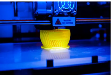
1.4.1 Fused Deposition Modeling (FDM)

Fused deposition modeling, also known as fused filament fabrication (FFF) in Figure 1.4-1, is an additive manufacturing technology commonly used to build up the 3D models.

(20)

FDM process is that a plastic filament supplies material to a temperature-controlled head and is heated to melt the material. Then the extrusion nozzle can moved in both horizontal and vertical directions by a numerically controlled mechanism and extrude a thermoplastic material layer by layer onto a workspace. Finally, the fused material is deposited layer by layer to build up the models.

Figure 1.4-1 The illustration of fused filament fabrication

Figure 1.4-2 Fused filament fabrication

(21)

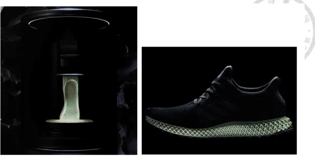
1.4.2 Stereo Lithography Apparatus (SLA) / Digital Light Processing (DLP)

The production procedure is done in a layer by layer fashion using photopolymerization, and it is a process by which light causes chains of molecules to link, forming polymers. In other words, using a light source (e.g. UV laser or projector) to cure liquid resin into hardened plastic. Those hardened plastics can construct the three dimensional entity step by step.

Figure 1.4-3 Compare the difference between SLA and DLP. SLA : selective exposure to light from laser. DLP : selective exposure to light from projector.

Figure 1.4-4 The illustration of Digital light processing (DLP)

(22)

1.4.3 Selective laser sintering (SLS)

A laser beam which is controlled by computer selectively fuses powdered material by scanning X and Y cross-sections on the surface of a powder bed. Using the laser as the power source to sinter powdered material binds the material together to create the three dimensional structure. Once the first layer is formed, the platform will drop usually by less than 0.1 mm and expose a new powder layer for the laser to fuse together. This process will continue again and again until the model has been completed.

Figure 1.4-5 The printing process of running shoe

Figure 1.4-6 The illustration of selective laser sintering

(23)

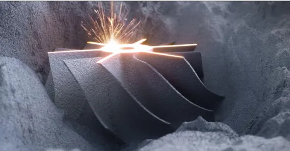
1.4.4 Selective laser melting (SLM)

Another method of 3D metal printing is selective laser melting (SLM), in which a high-powered laser fully melts each layer of metal powder rather than just sintering it.

Selective laser melting produces printed objects that are extremely dense and strong.

Figure 1.4-7 The result of selective laser sintering

Figure 1.4-8 The result of selective laser melting

(24)

1.4.5 Laser metal deposition (LMD)

Laser metal deposition (LMD) is an additive manufacturing process in which a laser beam forms a melt pool on a metallic substrate, into which powder is fed. The powder melts to form a deposit that is fusion-bonded to the substrate. The required model or geometry is built up in this way, layer by layer. Both the laser nozzle head can be manipulated using a gantry system or robotic arm.

Figure 1.4-9 the illustration of laser metal deposition (LMD)

Figure 1.4-10 Laser metal deposition (LMD)

(25)

1.4.6 Compare with additive manufacturing methods

Table 1 Compare with additive manufacturing methods

Material Advantages Disadvantages

FDM

1. PLA (Polylactic Acid)

2. ABS (Acrylonitrile Butadiene Styrene) 3. Nylon

4. Wax

1. Low maintenance costs

2. Equipment costs are inexpensive

3. The price of material is inexpensive

1. Axial strength is weak

2. Low accuracy 3. The surface has a

step structure 4. Need supports

SLA 1. Light-Curing Resins

1. Excellent surface quality

2. No need supports

1. Fewer types of materials can be used

2. The price of resin material is

expensive

SLS

1. Nylon 2. Polystyrene, 3. Metals including

steel, titanium, alloy mixtures, and composites 4. Green sand

1. Various types of materials can be used

2. No need supports 3. high accuracy

1. The surface roughness is granulated 2. Need post- processing 3. Expensive high

power laser 4. Dust pollution

SLM

1. Most metals including copper, aluminium, stainless steel, toll steel, cobalt chrome, titanium and tungsten.

1. Structural strength is high

2. No need supports 3. high accuracy

1. Expensive high power laser 2. Dust pollution 3. Expensive high

power laser

LMD

1. Most metals including titanium alloy, copper, aluminium,

1. Achieve rapid repair of damaged parts

2. high accuracy

1. Expensive high power laser

(26)

stainless steel, toll steel, cobalt chrome and tungsten.

3. the head can be manipulated using a gantry system or robotic arm

1.5 Thesis Organization

The thesis is organized as follows. Following this introduction, the experimental equipment and the 3D printer machine developed in our NTU-iCeiRA laboratory are introduced in Chapter 2. The hardware and software architectures are illustrated in the chapter. Moreover, the printing material is specified here. In Chapter 3 and Chapter 4, the highlighted processes in the additive and subtractive manufacturing are elaborated in detail. The additive manufacturing for multiple heterogeneous objects is discussed in Chapter 3. The fabrication procedures are illustrated in order, from the model extraction and analysis, collision consideration, printing strategy evaluation and planning location of multiple objects. In Chapter 4, carving 2D image onto 3D curved surface using hybrid additive and subtractive 3D printing approach is fully described. The proposed surface flattening algorithm that combines conformal mapping with optimal adjuster based on edge-lengths of the original mesh is illustrated. In Chapter 5, the experimental results about multiple heterogeneous objects fabrication and carving process are conducted on the 3D printer machine developed in our NTU-iCeiRA laboratory to evaluate the feasibilities of the proposed system. Analysis on the experimental results is also carried out to verify the proposed algorithms. Finally, the conclusions and future work are presented in Chapter 6.

(27)

Chapter 2 The Hardware and Software

2.1 Hardware

2.1.1 Mechanism Design

Both 3D printer and cutting tool are integrated in the gantry-type hybrid machine in Figure 2.1-1. The “hybrid” means that the printing part and carving part cooperate to complete the products. The machine not only executes additive and subtractive process separately but also combines two parts to do remanufacturing procedures of the same product. The cooperation can improve the accuracy of the production and the Figure 2.1-1 There are two parts on the gantry-type hybrid machine. Left side is the additive (3D printing) part while right side is subtractive (cutting) part.

(28)

repositioning process can be omitted at the same time.

2.1.2 Robot Coordinate System

The Denavit–Hartenberg parameters (D-H parameters) are the four parameters associated with a particular convention for attaching reference frames to the links of a spatial kinematic chain, or robot manipulator. Jacques Denavit and Richard Hartenberg introduced this convention in 1955 in order to standardize the coordinate frames for spatial linkages. The four parameters are necessary to fully describe the relationship between adjacent links and joints as follows:

D-H parameters in terms of the link frames:

 𝒅_𝒊 : the distance from 𝒙 ̂_𝒊−𝟏 to 𝒙 ̂_𝒊 measured along 𝒛 ̂_𝒊−𝟏

 𝜽_𝒊 : the angle from 𝒙 ̂_𝒊−𝟏 to 𝒙 ̂_𝒊 measured about 𝒛 ̂_𝒊−𝟏

 𝒂_𝒊 : the distance from 𝒛 ̂_𝒊−𝟏 to 𝒛 ̂_𝒊 measured along 𝒙 ̂_𝒊

 𝜶_𝒊 : the angle from 𝒛 ̂_𝒊−𝟏 to 𝒛 ̂_𝒊 measured about 𝒙 ̂_𝒊

The procedures for attaching coordinate on the link and identifying these four parameters are described as follows:

Link frame attachment procedures:

1. Identify the joint axes and imagine (or draw) infinite lines along them. For steps 2 through 5 below, consider two of these adjacent lines (at 𝒊^𝒕𝒉 and 𝒊 + 𝟏^𝒕𝒉 axes).

2. Identify the common perpendicular between them, or point of intersection. At the point of intersection, or at the point where the common perpendicular meets

(29)

the 𝒊^𝒕𝒉 axis, assign the link-frame as origin.

3. Assign the 𝒛 ̂_𝒊−𝟏 axis pointing along the 𝒊^𝒕𝒉 joint axis.

4. Assign the 𝒙 ̂_𝒊−𝟏 axis pointing along the common perpendicular, or, if the axes intersect, assign 𝒙 ̂_𝒊−𝟏 to be the normal to the plane containing the two axes.

5. Assign the 𝒚 ̂_𝒊−𝟏 axis to complete a right-hand coordinate system.

6. Assign frame {0} anywhere in the base as long as the 𝒛 ̂_𝟎 axis lies along the axis of motion of the first joint. The last coordinate (frame {n}) can be place anywhere in the end-effector as long as the 𝒙 ̂_𝒏 axis is normal to the 𝒛 ̂_𝒏−𝟏 axis.

7. Try to assign the link frame so as to cause as many linkage parameters as possible to become zero.

Figure 2.1-2 Definition of the D-H parameters

(30)

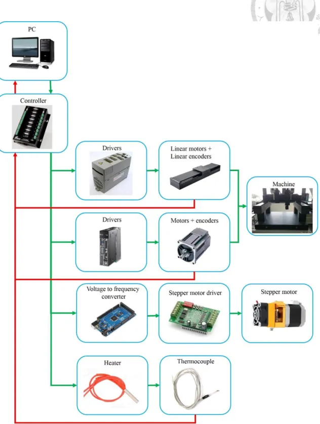
2.1.3 System Structure

Figure 2.1-3 Control architecture

(31)

The control architecture of the gantry-type machine system is shown as Figure 2.1-3.

The algorithm program is developed in PC base, then the algorithm is burned into UTC controller. And the voltage signal is sent into the driver to be transformed into current signal. While the machine is executing, the angle signal from encoder is sent back to UTC controller to achieve the feedback control. On the 3D printer part, the UTC controller also controls the speed of stepper motor and heater.

 Controller (UTC800P)

We use UTC controller as our operating kernel to manipulate the machine and implement the proposed algorithms. This controller provides some functions to control the machine smoothly and efficiently. Table 2 shows the specifications of controller, and the functions that contain communication, AD/DA(PWM), DNC, Blended Move and so on are often used.

Table 2 Specifications of UTC controller

Specifications UTC800V/P

CPU TMS320C32

Number of Control Axes 8

Figure 2.1-4 UTC controller

(32)

Driver (excluded)

Command Out 8V(16bit) / 8P(2M)

PLC/Motion Program 16 / 256 units

Communication RS-232x2/USB

Multi-Coordinate System 8

Look Ahead 1

Servo Algorithm PID+FF/ by Driver

Electrical Gear/Cam Table / Time base

On Board DI/DO 16 in / 8 out

AD/DA(PWM) 4(16bit)/4(12bit)

RAM 4Mb(16Mb)

Back Up RAM 4Mb Battery+Flash

System Clock Frequency (Hz) 40M

Servo Update Rate 1ms

Cutter Radius/ Lead screw Compensation N

Dual Encoder Feedback Y

DNC Y

Timers/Variables 8 / 4096

Hardware Capture Function Y

Password Security Y

Linear/Circular/ Screw Interpolation Y

Cubic Spline Interpolation Y

Scaling & Rotation Y

Blended Move Y

User-Defined G/M Code Y

 Controller (Arduino MEGA 2560)

This small controller is used as voltage to frequency converter to analyze the voltage signal of UTC controller, and will transform the voltage signal into the corresponding frequency output. The stepper motor driver needs to the clock to control the speed of

(33)

motor, but the UTC controller has only the voltage signal and it cannot output the different frequency. Therefore, we need the converter to transfer voltage into frequency signal. In the specifications, the digital I/O pins and analog input pins are often used with Arduino library.

Table 3 Specifications of Arduino MEGA 2560

Microcontroller ATmega2560

Operating Voltage 5V

Input Voltage (recommended) 7-12V

Input Voltage (limit) 6-20V

Digital I/O Pins 54 (of which 15 provide PWM output)

Analog Input Pins 16

DC Current per I/O Pin 20 mA

DC Current for 3.3V Pin 50 mA

Flash Memory 256 KB of which 8 KB used by bootloader

SRAM 8 KB

EEPROM 4 KB

Clock Speed 16 MHz

LED_BUILTIN 13

Length 101.52 mm

Width 53.3 mm

Weight 37 g

Figure 2.1-5 Arduino MEGA 2560

(34)

 Stepper Motor Driver (TB6560)

This driver can control the speed and direction of the stepper motor. The different position of dip switches have the different outputs. In the experiment, the running current that should be lower than the current rating of motor is set as 1.5A and the stop current is 50%. Excitation mode and decay setting are set as 1/16 and 0% respectively. The excitation mode can be said to be the resolution of the stepper motor. Therefore, excitation mode is set as a smaller value to let motor run smoothly.

Note :

1. 6 input terminals can be connected as common anode or cathode.

2. The normal input voltage is if it is more than 5V, than a series resistor is needed. This resistance is 1K case 12V and 2.4K case 24V.

3. When pulse is applied to CLK, the stepping motor will rotate, and stop when there is none, and the motor driver will change its current to the half mode as setting to hold the motor still.

4. Motor rotate clockwise when CW is low level and counterclockwise when CW is high level.

5. Motor is enable when EN is low level and disable when EN is high level.

Figure 2.1-6 stepper motor driver

(35)

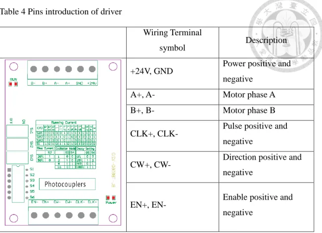
Table 4 Pins introduction of driver

Wiring Terminal

symbol Description

+24V, GND Power positive and negative

A+, A- Motor phase A

B+, B- Motor phase B

CLK+, CLK- Pulse positive and negative

CW+, CW- Direction positive and negative

EN+, EN- Enable positive and

negative

Table 5 Running current setting

Running Current

(A) 0.3 0.5 0.8 1 1.1 1.2 1.4 1.5 1.6 1.9 2 2.2 2.6 3

SW1 X X X X X O X O O O O O O O

SW2 X X O O O X O X X O X O O O

SW3 O O X X O X O O X X O O X O

S1 O X O X O O X O X O X O X X

(X : OFF O : ON)

Table 6 the setting about stop current, excitation mode and decay setting

Stop Current Excitation Mode Decay Setting

S2 Step S3 S4 Step S5 S6

20% ON Whole OFF OFF 0% OFF OFF

50% OFF Half ON OFF 25% ON OFF

(36)

1/8 ON ON 50% ON ON

1/16 OFF ON 100% OFF ON

 Stepper Motor

A stepper motor, also known as step motor or stepping motor, is a brushless DC electric motor, and the motor's position can then be commanded to move and hold at one of these steps without any feedback sensor. Its property to convert input pulses into the increment in the shaft position. Each pulse drives stepper motor to move a fixed angle that is depended on excitation mode of motor driver.

2.2 Software

2.2.1 STL (STereoLithography) Format

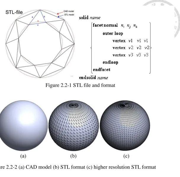
3D print models are typically distributed in a file format called STL. An STL file describes a raw unstructured triangulated surface by the unit normal and vertices (ordered by the right-hand rule) of the triangles using a three-dimensional Cartesian coordinate system. As a general rule, changing options such as chord tolerance or angular control will change the resolution on the STL file (see figure (b) and (c)).

Figure 2.1-7 Stepper Motor

(37)

2.2.2 Slicing Software

The process from the 3D file into the entity needs to do slicing processing step, and this step usually is implemented by slicing software or slicer. The slicing software takes 3D files (STL) and generates path information (G-Code) for a 3D Printer. These paths are written in G-Code, a program language, which describes the coordinates and instructions of the 3D printer’s nozzle when moving.

Figure 2.2-1 STL file and format

Figure 2.2-2 (a) CAD model (b) STL format (c) higher resolution STL format

(38)

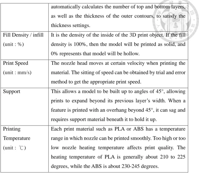
Table 7 the basic setting in the slicing software Instructions Description

Layer Height / Layer Thickness (unit : mm)

Layer thickness is a measure of the height of each successive addition of material in the additive manufacturing or 3D printing process in which layers are stacked. It is one of the essential technical characteristics of every 3D printer; the layer thickness is essentially the resolution of the z-axis, which is the vertical axis. If the sitting of layer thickness is smaller, the printed is more detailed and the higher the quality of the model but the longer the printing time.

Skin Thickness (unit : mm)

Whether the top, bottom, or side thickness of the model will be greater than or equal to this setting. The slicing software Figure 2.2-3 KISSlicer slicing software [27]

(39)

automatically calculates the number of top and bottom layers, as well as the thickness of the outer contours, to satisfy the thickness settings.

Fill Density / infill (unit : %)

It is the density of the inside of the 3D print object. If the fill density is 100%, then the model will be printed as solid, and 0% represents that model will be hollow.

Print Speed (unit : mm/s)

The nozzle head moves at certain velocity when printing the material. The sitting of speed can be obtained by trial and error method to get the appropriate print speed.

Support This allows a model to be built up to angles of 45°, allowing prints to expand beyond its previous layer’s width. When a feature is printed with an overhang beyond 45°, it can sag and requires support material beneath it to hold it up.

Printing Temperature (unit : ℃)

Each print material such as PLA or ABS has a temperature range in which nozzle can be printed smoothly. Too high or too low nozzle heating temperature affects print quality. The heating temperature of PLA is generally about 210 to 225 degrees, while the ABS is about 230-245 degrees.

G-Code format

Figure 2.2-4 G-Code file

(40)

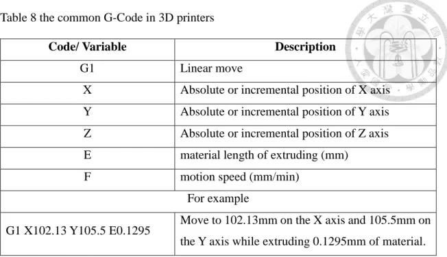
Table 8 the common G-Code in 3D printers

Code/ Variable Description

G1 Linear move

X Absolute or incremental position of X axis Y Absolute or incremental position of Y axis Z Absolute or incremental position of Z axis E material length of extruding (mm)

F motion speed (mm/min)

For example

G1 X102.13 Y105.5 E0.1295 Move to 102.13mm on the X axis and 105.5mm on the Y axis while extruding 0.1295mm of material.

2.2.3 Direct Numerical Control (DNC)

Direct numerical control (DNC), also known as distributed numerical control, is a common manufacturing term for networking CNC machine tools. On some CNC machine controllers, the available memory is too small to contain the machining program, so in this case the program is stored in a separate computer and sent directly to the machine.

With a direct numerical control system, the program will be run from a device (commonly a PC) connected to the machine’s communications port (the RS-232 port). In our system, the MATLAB is used in the host computer communicates with controller through the RS- 232 serial port. The computer will ask the controller how many instructions in the memory.

If the numbers of instructions in the memory are less than the critical value, the computer will send the following program to the controller. In this way, the controller can keep the amount of instructions to let the machine operate properly.

(41)

2.3 Material

2.3.1 PLA (Polylactic Acid)

Poly(lactic acid) or polylactic acid or polylactide (PLA) is a biodegradable and bioactive thermoplastic aliphatic polyester refined from renewable resources, such as corn starch (in the United States and Canada), tapioca roots, chips or starch (mostly in Asia), or sugarcane (in the rest of the world). This is why it is called “the green plastic”.

It’s widely used for packaging, such as food products, but of course you can also use it to print. In 2010, PLA had the second highest consumption volume of any bioplastic of the world.

Figure 2.2-5 Direct numerical control

(42)

2.3.2 ABS (Acrylonitrile Butadiene Styrene)

The most important mechanical properties of ABS are impact resistance and toughness. A variety of modifications can be made to improve impact resistance, toughness, and heat resistance. The impact resistance can be amplified by increasing the proportions of polybutadiene in relation to styrene and also acrylonitrile, although this causes changes in other properties. Impact resistance does not fall off rapidly at lower temperatures. Stability under load is excellent with limited loads. Thus, by changing the proportions of its components, ABS can be prepared in different grades. Two major categories could be ABS for extrusion and ABS for injection moulding, then good impact resistance. For the majority of applications, ABS can be used between −20 and 80 °C (−4 and 176 °F) as its mechanical properties vary with temperature.

Figure 2.3-1 PLA (Polylactic Acid)

(43)

2.3.3 PLA vs. ABS

Table 9 the difference between PLA and ABS

PLA ABS

Print temperature 190~220℃ 230~250℃

Plastic source Corn starch Petroleum extraction

Material hardness Strong hardness High toughness Fumes and smell Smells sweet Hot plastic fumes Degradability and

durability

Biodegradable Not biodegradable but can be easily recycled

Heated bed Not necessary Necessary

Figure 2.3-2 ABS (Acrylonitrile Butadiene Styrene)

(44)

Chapter 3 Multi-Heterogeneous Objects Fabrication for Additive Process

3.1 System Structure

Figure 3.1-1 system flowchart of additive manufacturing for multiple objects

(45)

The system can be distinguished into major four steps as follows.

 Step I. Model extraction and analysis

Each model is adjusted to appropriate posture after the STL file is imported.

 Step II. Collision consideration

This step needs to consider hardware specification to plan the printing path.

The nozzle can avoid colliding with the printed parts.

 Step III. Printing strategy evaluation

Calculate the relationship between models and workspace to determine the printing strategy. There are three strategies in the printing procedure.

Case 1: print the model layer by layer.

Case 2: print the model part by part.

Case 3: the workspace is large enough. Complete a model before move to the next one.

 Step IV. Planning location of multiple objects

Using the genetic algorithm solves the 2D packing problem to obtain the optimal solution.

3.2 Model Extraction and Analysis

In the additive manufacturing process, the construction of the support structure is necessary for some complex models. There are several reasons: on the one hand, support the structure of the object and enhance the structure stability between parts and build platforms. On the other hand, the support structure can prevent parts warping and reduce the failure rate in the printing process. Indeed, no one likes to support the

(46)

increases the additional printing time, cost, post-processing time and complexity.

Therefore, the optimization of the support structure is very important issue in 3D printing. To minimize and avoid the excessive use of the support structure as much as possible, it is necessary to have a good understanding about the geometry of the parts and the limitations of their construction.

For instance, the posture of model can be changed by rotating along the X, Y and Z axis (e.g. roll, pitch, yaw) to obtain proper position. In Figure 3.2-1and Figure 3.2-2, it is a simple case for us to easily comprehend the how to minimize and avoid the extra support structure. There are many support structures (the gray area in the Figure 3.2-1) under the table. The table is rotated 180 degrees along the X or Y axis to obtain the different result (see Figure 3.2-2), and support is not required to build up in the printing process. In the production time, the former needs to take 43.38 minutes to complete, while the latter only takes 30.95 minutes. Comparison between the two can be observed that the latter reduces the use of material and saves the 40.162% production time.

Therefore, the support optimization makes printing process more efficient.

Figure 3.2-1 table posture 1 (estimated build time: 43.38 minutes)

(47)

3.3 Collision Consideration

After the models are obtained, we talk about how to avoid colliding with the printed parts. There are two steps in this section. One is that the bounding box of each model is determined. Second, combining bounding box with the hardware information calculates the collision region for each model. The two steps are described in details as follows.

 Generate the bounding box for each model

After we get the model in the proper posture, we can flatten the model to the XY plane to obtain the 2D maximum contour (see Figure 3.3-1). In other words, the 2D contour of top view of model can also be represented. However, the 2D contours are usually irregular. The irregular contours are difficult to be applied to the following steps (e.g. 2D Packing Algorithm). The computational complexity of the algorithm is very high, and it means that the computer needs to pay the high cost on the time consumption and computational resource, but the results are not outstanding compared with approximate method.

Figure 3.2-2 table posture 2 (estimated build time: 30.95 minutes)

(48)

Therefore, the bounding rectangle is used to approximate the irregular contour (see Figure 3.3-1). This approximate method not only makes the problem simpler but also significantly reduces the computational complexity of the algorithm. In Figure 3.3-1, the red color rectangle without rotating is called original bounding rectangle.

The size of the original bounding rectangle may not be minimal. Therefore, we hope to calculate and obtain the minimum bounding rectangle to save printing workspace.

After that, we explain how to obtain the minimum bounding rectangle by seven steps as follows.

1. Compute convex hull of the object, then get a polygon.

2. Find all four extreme points for the polygon. Compute the area of the rectangle determined by the four lines, and keep as minimum.

3. Rotate the lines clockwise until one of them coincides with an edge of its polygon.

Figure 3.3-1 the left image is Moai model. Top right is the top view of the Moai model and lower right is the irregular contour.

(49)

4. Compute the area of the new rectangle, and compare it to the current minimum area.

5. Update the minimum if necessary, and keep track of the rectangle, determine the minimum.

6. Repeat steps 3 - 5 until all edges have been processed.

7. Output the minimum area enclosing rectangle.

The result that is shown in Figure 3.3-2 displays that the shape of object is surrounded by two rectangles. The red rectangle is original bounding rectangle and its area is equal to 588.816 𝑐𝑚², while the area of green rectangle equals to 529 𝑐𝑚². Therefore, the green rectangle is called as the minimum bounding rectangle (MBR).

 Calculate the collision region

The collision region is inferred from hardware information. If the nozzle moves Figure 3.3-2 red rectangle is original bounding rectangle

(Area : 588.816 𝑐𝑚²), and green is minimum bounding rectangle (Area : 529 𝑐𝑚²)

(50)

into the collision region, the printed parts may be collided and damaged by the extrusion nozzle. Therefore, how to decide the size and position of the collision region is an important issue in the printing process. We decide three situation about the collision region in Figure 3.3-3. And the nozzle tip is defined as the origin point.

Situation 1: the region is in the red dashed rectangle. It is close to the nozzle, we can express as Equation (3-1).

𝑙_𝑙< 𝑥 < 𝑙_𝑟, −𝑛_𝑑

2 < 𝑦 <𝑛_𝑑

2 (3-1)

Situation 2: the region that is in the blue dashed rectangle excluding the area of the red rectangle can be represented as the Equation (3-2).

𝑝_𝑙< 𝑥 < 𝑙_𝑙 𝑜𝑟 𝑙_𝑟 < 𝑥 < 𝑝_𝑟, 𝑛_𝑑

2 > 𝑦 > −𝑛_𝑑

2 (3-2)

Situation 3: the area is other region which is not in red and blue dashed rectangle, and the conditions can be described as the following inequality.

𝑥 < 𝑝_𝑙 𝑜𝑟 𝑥 > 𝑝_𝑟, 𝑛_𝑑

2 < |𝑦| (3-3)

Figure 3.3-3 The illustration about collision region definition

(51)

After the minimum bounding rectangle of models are obtained, these rectangles are modified by collision conditions. In other words, expanding the rectangles are equal to increasing the safety distance between the printed parts and the nozzle in the printing process. We can determine the size of bounding box with collision conditions by using the relationship of relative motion between the nozzle and the printed model. In Figure 3.3-4, the dark gray area is maximum contour of model. The red, blue and gray rectangle are corresponded to situation 1, 2 and 3 respectively. Finally, the collision regions are defined and calculated simply. In order to clearly explain later, the 𝑖th collision region is defined as 𝑅_𝑖 = (𝑥, 𝑦, 𝑤, ℎ), where (𝑥, 𝑦) is the coordinate of the center of the rectangle and 𝑤 and ℎ are the width and height of the rectangle respectively.

Figure 3.3-4 the dark gray area is maximum contour of model, and the green is minimum bounding rectangle. The red, blue and gray rectangle are corresponded to situation 1, 2 and 3 respectively.

(52)

3.4 Printing Strategy Evaluation

This step is how to choose the proper printing strategy for multiple objects according to the relationship between the size of workspace and area of collision regions. The size of workspace is decided as the set of points that can be reached by end‐effector of machine, and the three collision regions that are mentioned above have been obtained. Our objective is to reduce production time and increase fabrication efficiency. The key is “transition travel” where the nozzle moves along among the objects without printing (show red color in Figure 3.4-1). Proposed algorithm attempts to minimize the transition travel distance as well as to improve motion path. Not only is some energy saved, but also the total manufacturing time is reduced directly.

As a result, we can sum up three strategies by using information about the size of workspace and collision regions. Three cases are described in detail as follows.

Figure 3.4-1 the blue line represents the printing paths and the red line is transition paths.

(53)

Table 10 the production time analysis on the printing and transition paths (model information: height is 100mm, number of layers is 392)

Case1 Case2 Case3

Printing time(min) 94.64 (72.89%) 94.64 (98.83%) 94.64 (99.62%) Transition

time(min)

35.198 (27.11%) 1.1216 (1.17%) 0.3582 (0.38%)

Total time(min) 129.838 95.7616 94.9982

Case 1: print the models layer by layer.

The common slicing software uses layer by layer planning method to do printing path planning for multiple objects. Therefore, when multiple objects are printed at the same time, the nozzle moves among objects and always increases enormous distance of the transition travel. We use two 101 models as an example in order to clearly analyze the results shown in Figure 3.4-1. In the printing process, the nozzle moves to the next model after the first layer of first model is completed. Then, the nozzle returns to first model again after the first layer of another model is also completed. The process is finished when the models are built up.

Case 2: print the models part by part.

Optimizing the printing strategy reduces a lot of transition paths to increase printing efficiency and save extra energy. Printing the two object shows the process as follows. At first, print the model until appropriate height and move to next one. The second step is to print some layers until proper height, then return the first step. The recursive processing

(54)

is interrupted when the objects are completed. Obviously, the number of transition path between two objects is far less than the common slicing methods.

Case 3: complete the models one by one.

The model can be completed then move to the next one until all models are built up.

This method is the most efficient and fastest in the three strategies. It can not only reduce much production time but also save more energy. However, the condition is that the workspace needs to be large enough so that the nozzle does not hit other printed objects during the printing process. The case 3 of Figure 3.4-1 shows the a few transition paths compared with the case 1 or case 2.

Therefore, the printing strategy is determined by the size of workspace and the area of minimum bounding rectangles.

(55)

3.5 Planning Location of Multiple Objects

After the printing strategy is determined, the location of models are optimized to reduce the length of transition paths. We apply the 2D packing algorithm to arrange the collision regions to be optimized for placement. The 2D packing algorithm is based on genetic algorithm (GA), and the cost function of genetic algorithm is set as the sum of the distance among objects.

3.5.1 2D Packing Algorithm

The rectangular packing problem, also known as the two-dimensional (2D) packing problem, is a well-known combinatorial optimization problem which is the problem of orthogonally packing a given set of rectangles into a two-dimensional rectangular bin.

Packing problems are concerned with finding a proper arrangement of multiple items in larger containing region. The objective of the allocation process is to minimize the cost function that is defined by ourselves.

The packing process has to ensure that there is no overlap between the items and no items can beyond the confine of workspace. These restrictions can be expressed as

𝐴_𝑖 ∩ 𝐴_𝑗 = ∅, 𝑖 ≠ 𝑗, ∀𝐴_𝑖, 𝐴_𝑗, 𝑖 = 1, … , 𝑛, 𝑗 = 1, … , 𝑛 (3-4) and

𝐴_𝑖∩ 𝐴_𝑤 = 𝐴_𝑖, ∀𝐴_𝑖, 𝑖 = 1, … , 𝑛. (3-5) where 𝐴_𝑤 is the area of the workspace, as well as 𝐴_𝑖 and 𝐴_𝑗 are the area of the collision regions. The number of collision regions is 𝑛.

Figure 3.5-1 shows the illustration of the packing problem, and the different

(56)

rectangles are represented as collision regions that are mentioned above. The block rectangle is a workspace. After that, we use the genetic algorithm to solve the packing problem.

3.5.2 Genetic Algorithm

Genetic algorithm (GA) is a metaheuristic inspired by the process of natural selection that belongs to the larger class of evolutionary algorithms (EA). The main core concept is natural selection and evolutionary processes. This algorithm is used to generate high quality solutions to obtain the best solutions by relying on bio-inspired operators such as selection, crossover and mutation. A population of candidate solutions, also called individuals, chromosomes or phenotypes, is evolved toward better solutions through multiple iterations. The evolution usually starts from a population of randomly generated individuals, and is an iterative process, with the population in each iteration called a

Figure 3.5-1 the illustration of two-dimensional packing problem.