邊緣裝置上的高效能隨時分類

(1)

國立臺灣大學電機資訊學院電機工程學系碩士論文

Department of Electrical Engineering

College of Electrical Engineering and Computer Science

National Taiwan University Master Thesis

邊緣裝置上的高效能隨時分類

Efficient Anytime Classification on Edge Devices

林士彰 Shih-Chang Lin

指導教授：郭斯彥博士 Advisor: Sy-Yen Kuo, Ph.D.

中華民國 109 年 7 月 July 2020

(2)

(3)

誌謝

能完成這篇論文，要先感謝我的指導教授郭斯彥教授，教授提供了我完善的環境和豐富的研究資源，讓我能順利撰寫及完成實驗，以及要感謝袁世一教授，

在例行性的會議報告中給予我許多改善建議，讓論文得以更加完整。還要感謝陳韋廷學長、謝宙穎同學、吳宜凡同學、黃俊穎同學，在討論時提供我許多想法與建議，最後還要感謝實驗室的每一位成員對我的協助、支持與鼓勵，讓我能順利完成論文。

(4)

摘要

近年來隨著物聯網、自駕車等應用的發展，邊緣計算越來越為重要。而這些技術的發展與神經網路有著重要的關聯，許多應用都將使用到神經網路。我們發現在邊緣裝置上可能會有計算能力較低的特性，也可能在能源上有所限制或是透過外部的其他資源來獲得能量，且有許多邊緣裝置都需要使用在即時的應用中。因此我們提出了幾項方法來針對神經網路的輸入做處理，以大量減少神經網路所需的計算量，並嘗試保持神經網路的準確率。我們針對我們的方法來搭配資料集做實驗，

接著對實驗結果做分析與討論，最後在邊緣裝置的使用上提出相關的建議。在三個資料集的實驗中，我們最好的方法至少可以減少網路架構 50%以上的 FLOPs。表明我們的方法將可以依照邊緣裝置的情境來解決邊緣裝置計算能力低、能源有限、

即時應用等問題。

關鍵字：邊緣運算、邊緣裝置、隨時分類、高效分類、高效網路架構

(5)

Abstract

In recent years, with the development of applications of the Internet of Things, Self- driving cars, and other fields, Edge Computing has become increasingly important. The development of these technologies has an important relationship with neural networks, and many applications will use neural networks. We found that edge devices may have lower computing capability, or may have limited resources or obtain energy through other external resources, and many edge devices need to be used in real-time applications.

Therefore, we propose several methods to process the input of the neural network to reduce the amount of calculation required by the neural network and try to maintain the accuracy of the neural network. We will experiment with the dataset according to our method, then analyze and discuss the experimental results, and finally put forward relevant suggestions on the use of edge devices. In the experiment of the three datasets, our best method can reduce the FLOPs of the network architecture by at least 50%. It shows that our method can solve the problems of low calculation capacity, limited energy, and real-time applications of edge devices according to the situation of edge devices.

Keywords: Edge Computing, Edge Device, Anytime Prediction, Efficient

Classification, Efficient Network Architecture

(6)

List of Figures

Figure 1: MSDNet Architecture... 8

Figure 2: Variational Autoencoder (VAE) Architecture ... 9

Figure 3: Flow chart of Edge Device ... 10

Figure 4: Wavelet transform result ... 12

Figure 5: OpenCV Resize result ... 14

Figure 6: Pre-training VAE architecture ... 16

Figure 7: VAE + MSDNet architecture ... 16

Figure 8: Mini NN architecture ... 18

Figure 9: Conv3 with shortcut architecture ... 19

Figure 10: Classifier architecture in MSDNet ... 21

Figure 11: The percentage of FLOP required for each block prediction in CIFAR- 10 relative to the original method ... 27

Figure 12: CIFAR-10 dataset experiment results ... 28

Figure 13: The percentage of FLOP required for each block prediction in CIFAR- 100 relative to the original method ... 31

Figure 14: CIFAR-100 dataset experiment results ... 32

Figure 15: The percentage of FLOP required for each block prediction in ImageNet relative to the original method ... 34

(8)

Figure 16: ImageNet dataset experiment results ... 35

(9)

List of Tables

Table 1: OpneCV Resize interpolation option description ... 13

Table 2: Details of the experimental dataset ... 23

Table 3: Training parameter settings ... 24

Table 4: The accuracy of CIFAR-10 after training ... 26

Table 5: FLOPs required for each block prediction in CIFAR-10 ... 27

Table 6: The accuracy of CIFAR-100 after training ... 29

Table 7: FLOPs required for each block prediction in CIFAR-100 ... 30

Table 8: The accuracy of ImageNet after training ... 33

Table 9: FLOPs required for each block prediction in ImageNet ... 34

(10)

Chapter 1 Introduction

In recent years, with the development of applications of the Internet of Things, Self- driving cars, and other fields, Edge Computing has become increasingly important. There are more and more applications for real-time processing and analysis after collecting data at the edge device. These applications usually require a very short latency to meet the needs of the application. Through the application of edge devices, we will be able to reduce the bandwidth and energy consumption of transferring data to the cloud. However, applications in the Internet of Things, self-driving cars, and other fields can develop rapidly, because people have made a great breakthrough (neural networks) in the Computer Vision and Pattern Recognition field. Examples we can know are as follows:

[2] use data from human driving records to train an end-to-end convolutional neural network, [3] get a small number of key perception indicators that directly relate to the affordance of a road/traffic state for driving from input images, then make driving decisions, [4] use deep neural network for PCB(Printed circuit board) defect classification and improve defect recognition rate, [5] classification of skin cancer through the deep neural network, [6] using neural network technology, the first program to defeat a world

(11)

In 2009, people established the ILSVRC [10] dataset classification competition in the field of neural networks, with the goal of achieving the highest accuracy in the dataset.

This competition has attracted people's research and promoted the development of neural networks. Convolutional neural network (CNN) has achieved amazing results in the competition, so the convolutional neural network (CNN) has become the main network architecture in current classification applications. In the competition, the Convolutional neural network, which is intensively calculated with deep layers, obtains good results, such as these networks that won the championship of the year: GoogLeNet[11] in 2014, ResNet[12] in 2015, SeNet[13] in 2017. Although some of the lighter networks have been researched at present, we still think that these lighter network applications will consume too much computing resources on the edge devices, so that they consume too much energy.

We need to consider the mobile phone devices, Internet of Things devices, and even Energy harvesting devices that may be used in practical applications. Below we will give examples of several devices that need to be applied to neural networks to illustrate:

(1) Devices with lower calculation capacity ： In an edge computing device, the calculation usually uses the CPU, and the calculation capability is not too high, nor can the GPU be used to accelerate the operation. Therefore, if a network with a large structure is used, too many resources will be occupied. Even if the network structure is too large, the memory will be insufficient and the calculation cannot be completed.

(12)

Such a device may be a Raspberry Pi or a chip with a smaller amount of calculation.

(2) Real-time application：When we need an application that responds in real-time, if the network architecture and network calculations are too large, it may take a lot of time to complete the calculation, so there will be no way to react in real-time, which may cause a large latency or impact on the entire application. Such a device may be a computing unit located in a Self-driving car.

(3) Energy limited devices：Devices with limited energy usually obtain energy through other external resources (such as solar energy) and then perform calculations, so they are often faced with the possibility of power failure or machine shutdown. In this case, if half of the calculations do not have a result and need to be powered off or need to store the current state and then shut down, it may cause this calculation to gain nothing and waste the previously collected energy. Such devices may be a large number of miniature sensors scattered outdoors or satellite devices in space.

Based on the above example, we think that if you want to use a neural network to complete applications in an edge computing environment, the neural network architecture requires the following two characteristics:

(1) Lower FLOPs(floating point operations)：If we only need less FLOPs to complete the calculation and can maintain a certain accuracy, it will be able to complete the

(13)

calculation in the device with lower calculation capacity. It can also reduce latencies in real-time applications and reduce energy waste in devices with limited energy.

(2) Anytime Prediction：If our neural network can output the results and store the results after the calculation amount reaches a certain FLOPs, this will reduce the waste of energy in devices with limited energy. Even further, we hope that the output of the middle layer can leave the calculation of the neural network if it exceeds a certain threshold. In this way, more energy consumption can be reduced, and some parts of the network can be calculated in devices with lower computing power. In real-time applications, it will respond more quickly and reduce more latencies.

In 2017, [1] proposed MULTI-SCALE DENSE NETWORKS (MSDNet), which provided the output of the middle layer, and would reduce the impact on the final output.

MSDNet has reached a certain accuracy on the Cifar10, Cifar100 [9], and ILSVRC 2012 (ImageNet) [10] datasets, which is the state-of-the-art technology in the field of Anytime Prediction. But we think that there are still too many FLOPs in the MSDNet network, so we hope to reduce FLOPs and maintain the accuracy of the neural network, making the neural network more suitable for use on edge devices.

In this thesis, we hope to process the input of the network to greatly reduce the overall FLOPs of the neural network. We will try various methods to reduce the input data of the

(14)

neural network, including CNN, Variational Autoencoder(VAE) [7][8], wavelet transform, traditional image processing algorithm (resize) and other methods to pre- process the input data, and then analyze and discuss the results. Finally, we will summarize which method is most suitable for the edge device. Our main contributions are: (1) propose a network architecture that can greatly reduce FLOPs but maintain a certain accuracy (2) propose a solution to the problems that edge devices may face low calculation capacity, limited energy, real-time applications, etc. (3) provide experimental data for future related research as a reference.

(15)

Chapter 2 Related Works

Some previous work was to make the network efficient, including [14] through pruning [15], quantization, and finally using Huffman coding to increase the calculation speed and reduce energy consumption. In addition, other related work on pruning and quantization is [16][17][18][19][20][21]. [16][17] reduce calculation cost through pruning filters, [18] reduce input channel through a two-step algorithm to effectively prune each layer to accelerate prediction speed. [19] reduces the memory size and accesses by binarizing the weights and uses Sign Operation to speed up the calculation.

[20] is binarizing the weights and inputs to reduce the memory size and accesses of the model and accelerate the model. [21] define the filter-level pruning problem of the binary neural network, and proposed to prune the filters in the main/subsidiary network framework, where the main network is the same as normal network, and the subsidiary is the filter selector on the main network. What is different from us is that we hope to propose a method without modifying each different network architecture. But these technologies can be combined with our method in the future, so that the network architecture can be further reduced, and thus more FLOPs can be reduced. To make the

(16)

neural network have lower FLOPs and can be predicted at any time, we will use the state- of-the-art network architecture (MSDNet) in the current Anytime prediction field and combine it with our proposed method to achieve our goal.

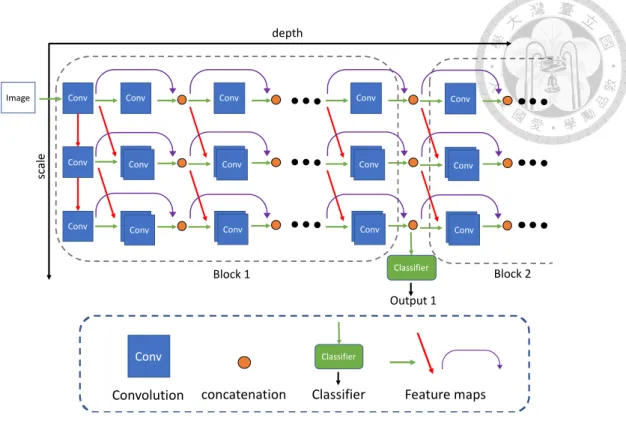
MSDNet is an anytime prediction neural network designed in combination with DenseNet [22]. The architecture of the network is shown in Figure 1. MSDNet is the neural network architecture of the array. The horizontal direction is depth, which is the same as a general neural network. More specifically, the vertical direction is scale, to increase the acquired features, so that the previous prediction results can be better. The classifier in the MSDNet network architecture uses blocks as a unit, followed by a classifier after each block to output prediction results. In addition to the horizontal first layer and the vertical first layer, each input comes from the previous layer in the horizontal direction and the oblique front layer. However, the concept of DenseNet is used in the horizontal direction to optimize for early classifiers.

(17)

Figure 1: MSDNet Architecture

In addition, in our method, which also refers to the network architecture of ResNet [12][24], we use a similar shortcut structure to try to increase our accuracy. In addition, Variational Autoencoder (VAE) network architecture is also used. Variational Autoencoder (VAE) was proposed in 2014 [7] and 2016 [8], and is usually used as a method of compressing data. The concept is shown in Figure 2. The concept is shown in Figure 2. We take an image or a series of codes as input, and then encode through Encoder to generate a Code. This Code is the feature and can be restored to an image through the Decoder. Theoretically, although the restored image has losses, it should be very similar

Conv

ConvConv

Conv

ConvConv ConvConv

ConvConv

Conv

ConvConv

Conv

ConvConv

Classifier

Output 1

Block 1 Block 2

depth

scale

Image

Conv

Convolution concatenation

Classifier

Classifier Feature maps

(18)

to the original image under the recognition of the human eye. The detailed architecture and usage method will be introduced in Chapter3.

Figure 2: Variational Autoencoder (VAE) Architecture. Input image source: CIFAR-10[9]

dataset.

Encoder Decoder

Input code Output

(19)

Chapter 3 Method

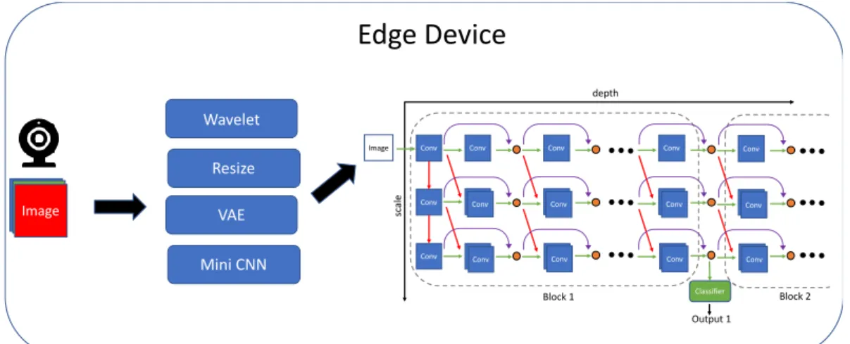
Our overall method is shown in Figure 3. We assume that the edge device can obtain the original data through the sensor or camera, and this data will be a color image with three channels of RGB. Then we pre-process this color image to reduce the input image to 1/4, and then input the reduced image into MSDNet. Finally, the corresponding output is made according to the conditions (energy, calculation capacity, memory, etc.) of each edge device. In this case, the overall calculated FLOPs will theoretically be reduced by about 75% compared to the original FLOPs.

Figure 3: Flow chart of Edge Device

Conv

Conv Conv

ConvConv

Conv

ConvConv ConvConv

ConvConv

Conv

ConvConv

Conv

ConvConv

Classifier Output 1

Block 1 Block 2

depth

scale

Image

Wavelet Resize

VAE Mini CNN

Edge Device

(20)

3.1 Pre-Process

3.1.1 Wavelet Transform

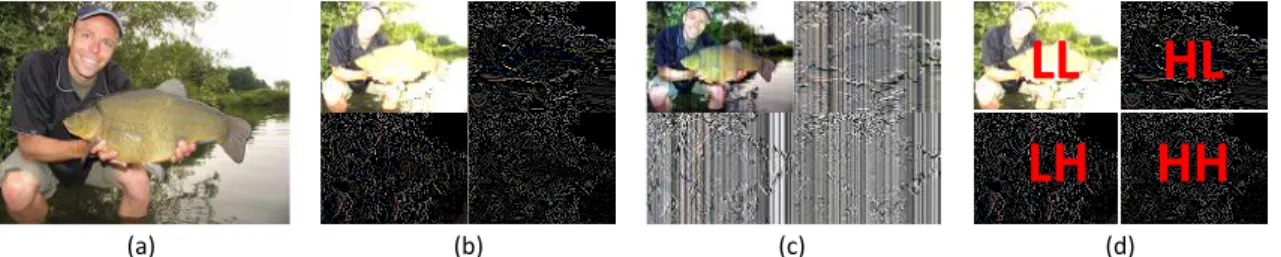
In the pre-processing, we will use the Haar family to do the 2D discrete wavelet transform on the input image, and the result is shown in Figure 4(b). But in the process of using, we will have the following problems:

Problem 1: We cannot directly do the 2D discrete wavelet transform on RGB color

images.

Solution 1: Under normal circumstances, we cannot directly do the 2D discrete wavelet

transform on images with more than 2 channels. Therefore, we split the original image into the three RGB channels, and do the 2D discrete wavelet transform on the three RGB channels respectively, and finally merge the three RGB channels after the 2D discrete wavelet transform.

Problem 2: The pixel value after wavelet transform exceeds 255.

Solution 2: We will do the MinMaxScaler function for each column of the image, and

limit the value of each pixel to 0 ~ 255. The formula is as follows:

𝑋_{𝑠𝑐𝑎𝑙𝑒𝑑} = (𝑋 − 𝑋. min(𝑎𝑥𝑖𝑠 = 0))

(𝑋. 𝑚𝑎𝑥(𝑎𝑥𝑖𝑠 = 0) − 𝑋. 𝑚𝑖𝑥(𝑎𝑥𝑖𝑠 = 0))× (𝑚𝑎𝑥 − 𝑚𝑖𝑥) + 𝑚𝑖𝑛

(21)

X is the current value to be processed in each column, X.min (axis = 0) represents the

minimum value in each column, X.max (axis = 0) represents the maximum value in each column, max means the maximum value of the range we set, and min means the minimum value of the range we set. The final result is shown in Figure 4 (c).

Problem 3: Using 2D discrete wavelet transform for the input image, we will get four

subbands of LL, HL, LH, and HH (as shown in Figure 4 (d)), where L represents low frequency and H represents high frequency. The problem is which part is the one we are going to input into the next stage?

Solution 3: LL is the most important frequency band, it retains the most information of

the original image, so we will choose the LL frequency band alone. In addition, in order to enhance the feature of the image, we will also try to add the information of other frequency bands to the LL frequency band. The detailed test results will be presented in the experiment.

Figure 4: Wavelet transform result. (a) Original image (b) the result of the image after wavelet transformation (c) the result of the image after the wavelet transformation and then processed by the MinMaxScaler function (d) frequency band position of the image after wavelet transformation. Input image source: ILSVRC 2012[10] dataset.

(b) (c) (d)

HL HH LH

LL

(a)

(22)

3.1.2 Resize

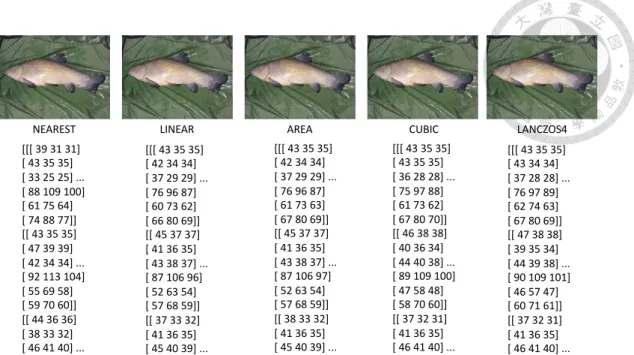
We will use the resize method in OpenCV to reduce the image to 1/4 of the original image, which will use different interpolation options for the image. The description of the interpolation option in the Resize of OpenCV is shown in Table 1, and the processed result is shown in Figure 5. We can find that it is difficult to find the difference directly with the human eye, but after we show the pixels of each part of the image below the picture, we can see that there are still slight differences. Therefore, the use of different interpolation options may still affect the neural network. The results of the detailed impact will be presented in the experimental chapter.

Interpolation option Option description

INTER_NEAREST a nearest-neighbor interpolation

INTER_LINEAR a bilinear interpolation (used by default)

INTER_AREA resampling using pixel area relation. It may be a preferred method for image decimation, as it gives moire’-free results. But when the image is zoomed, it is similar to the INTER_NEAREST method.

INTER_CUBIC a bicubic interpolation over 4x4 pixel neighborhood INTER_LANCZOS4 a Lanczos interpolation over 8x8 pixel neighborhood Table 1: OpneCV Resize interpolation option description [23]

(23)

Figure 5: OpenCV Resize result. The image is processed according to different Resize interpolation options, the upper part is the image result, and the lower part is part of the pixels in each image. Input image source: ILSVRC 2012[10] dataset.

AREA CUBIC LANCZOS4

LINEAR NEAREST

[[[ 39 31 31]

[ 43 35 35]

[ 33 25 25] ...

[ 88 109 100]

[ 61 75 64]

[ 74 88 77]]

[[ 43 35 35]

[ 47 39 39]

[ 42 34 34] ...

[ 92 113 104]

[ 55 69 58]

[ 59 70 60]]

[[ 44 36 36]

[ 38 33 32]

[ 46 41 40] ...

[[[ 43 35 35]

[ 42 34 34]

[ 37 29 29] ...

[ 76 96 87]

[ 61 73 63]

[ 67 80 69]]

[[ 45 37 37]

[ 41 36 35]

[ 43 38 37] ...

[ 87 106 97]

[ 52 63 54]

[ 57 68 59]]

[[ 38 33 32]

[ 41 36 35]

[ 45 40 39] ...

[[[ 43 35 35]

[ 43 35 35]

[ 36 28 28] ...

[ 75 97 88]

[ 61 73 62]

[ 67 80 70]]

[[ 46 38 38]

[ 40 36 34]

[ 44 40 38] ...

[ 89 109 100]

[ 47 58 48]

[ 58 70 60]]

[[ 37 32 31]

[ 41 36 35]

[ 46 41 40] ...

[[[ 43 35 35]

[ 43 34 34]

[ 37 28 28] ...

[ 76 97 89]

[ 62 74 63]

[ 67 80 69]]

[[ 47 38 38]

[ 39 35 34]

[ 44 39 38] ...

[ 90 109 101]

[ 46 57 47]

[ 60 71 61]]

[[ 37 32 31]

[ 41 36 35]

[ 46 41 40] ...

[[[ 43 35 35]

[ 42 34 34]

[ 37 29 29] ...

[ 76 96 87]

[ 60 73 62]

[ 66 80 69]]

[[ 45 37 37]

[ 41 36 35]

[ 43 38 37] ...

[ 87 106 96]

[ 52 63 54]

[ 57 68 59]]

[[ 37 33 32]

[ 41 36 35]

[ 45 40 39] ...

(24)

3.1.3 Variational Autoencoder (VAE)

The Code generated by VAE(Variational Autoencoder) through Encoder can restore most of the original image, so we believe that Code has features that can be used as classification conditions. In this method, we use a pre-trained VAE network architecture to combine MSDNet. Our pre-trained VAE network architecture is shown in Figure 6. In the Encoder part, it contains four layers of Conv, and then connects two fully connected layers respectively, and performs the calculation of the following formula:

𝑐𝑜𝑑𝑒 = 𝑒𝑥𝑝(σ_𝑖 × 0.5) × 𝑒_𝑖+ 𝑚_𝑖

The output of the fully connected hierarchy is mi and σi, ei is a normally distributed random number, the Code is generated after the operation, and finally the Decoder is used to restore the Code to the image. Decoder contains a fully connected layer and four DeConv. In our method, we use the Code after Encoder as the input of MSDNet. The overall architecture is shown in Figure 7.

(25)

Figure 6: Pre-training VAE architecture. Input image source: CIFAR-10[9] dataset.

3x3 conv, 3->32, stride 1

3x3 conv, 32->64 , stride 1

3x3 conv, 64->128 , stride 1

4x4 conv, 128->256 , stride 2

Fc 65536->768(16*16*3)

Fc 768->65536(16*16*256)

Fc 65536->768(16*16*3)

� � � � ×0.5 �

�

3x3 deconv, 64->32 , stride 1 3x3 deconv, 128->64 , stride 1 4x4 deconv, 256->128, stride 2

3x3 deconv, 32->3, , stride 2 X

+

Decoder Encoder

Input

Output code

ReLU ReLU ReLU ReLU ReLU

ReLU

ReLU ReLU

Conv

Conv Conv

ConvConv

Conv

ConvConv ConvConv

ConvConv

Conv

ConvConv

Conv

ConvConv

Classifier Output 1

Block 1 Block 2

depth

scale

Image

3x3 conv, 3->32, stride 1 3x3 conv, 32->64, stride 1 3x3 conv, 64->128, stride 1 4x4 conv, 128->256, stride 2 Fc 65536->768(16*16*3) Fc 768->65536(16*16*256)

Fc 65536->768(16*16*3) !"#$!×0.5)!!! 3x3 deconv, 64->32, stride 1

3x3 deconv, 128->64, stride 1

4x4 deconv, 256->128, stride 2 3x3 deconv, 32->3, , stride 2

X + Decoder

Encoder

Input Output

code ReLU

ReLU

ReLU ReLU ReLU ReLUReLU

(26)

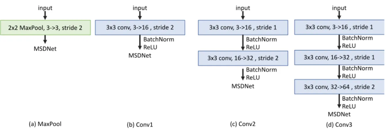
3.1.4 Mini NN

We also try to reduce the input image with a small neural network architecture before inputting into MSDNet, to reduce the FLOPs required by the neural network. These network structures will be trained together with MSDNet. Below we will introduce the network architecture we have tried one by one:

(a) Maxpool: Add a MaxPool layer in front of MSDNet, as shown in Figure 8 (a), use 2

* 2 kernel size, stride is set to 2, and the output image size is 3 (channel) * 16 * 16.

(b) Conv1: Add a Convolution layer in front of MSDNet, as shown in Figure 8 (b), use 3 * 3 kernel size, stride is set to 2, and add BatchNorm and ReLU layer behind the Convolution layer, the output image size is 16 (channel) * 16 * 16.

(c) Conv2: Add two Convolution layers in front of MSDNet. As shown in Figure 8 (c), both Convolution layers use 3 * 3 kernel size. The stride of the first Convolution layers is set to 1, and the stride of the second Convolution layer is set to 2. The BatchNorm and ReLU layers are added after each Convolution layer, and the output image size is 32 (channel) * 16 * 16.

(d) Conv3: Add three Convolution layers in front of MSDNet. As shown in Figure 8 (d), the three Convolution layers all use 3 * 3 kernel size. The stride of the first and second Convolution layers is set to 1, and the stride of the third Convolution layer is set to 2.

The BatchNorm and ReLU layers are added after each Convolution layer, and the

(27)

output image size is 64 (channel) * 16 * 16.

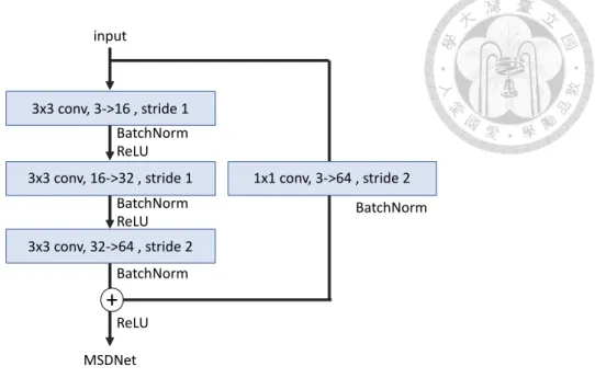
(e) Conv3 with shortcut: Add three Convolution layers on the left and a shortcut on the right in front of MSDNet. As shown in Figure 9, the three Convolution layers on the left all use 3 * 3 kernel size. The stride of the first and second Convolution layers is set to 1, the stride of the third Convolution layer is set to 2, and the BatchNorm and ReLU layers are added after the Convolution layers of the first and second layers, but the last layer of the Convolution layer only uses BatchNorm. Then add the shortcut on the right. The shortcut is a Convolution layer with 1 * 1 kernel size, stride is set to 2, and the results of the left and right sides are added before using ReLU. The final output image size is 64 (channel) * 16 * 16.

Figure 8: Mini NN architecture. (a) MaxPool (b) Conv1 (c) Conv2 (d) Conv3

2x2 MaxPool, 3->3, stride 2 input

MSDNet

(a) MaxPool (b) Conv1 (c) Conv2 (d) Conv3

3x3 conv, 3->16 , stride 2 input

MSDNet BatchNorm ReLU

MSDNet 3x3 conv, 16->32 , stride 2

BatchNorm ReLU

MSDNet 3x3 conv, 16->32 , stride 1

3x3 conv, 32->64 , stride 2 BatchNorm ReLU BatchNorm ReLU BatchNorm ReLU

(28)

Figure 9: Conv3 with shortcut architecture

MSDNet

3x3 conv, 16->32 , stride 1

3x3 conv, 32->64 , stride 2 BatchNorm BatchNorm ReLU BatchNorm ReLU

1x1 conv, 3->64 , stride 2 BatchNorm

ReLU

+

(29)

3.2 MSDNet architecture modification

Because we reduced the input to 1/4 size and also changed the input channel, we need to modify the network architecture. We will discuss the parts that need to be modified separately.

3.2.1 Input channel size modification

In the three parts of the wavelet transform, Resize, and VAE, only the length and width of the input are changed, and the channel has not changed, so no modification is needed in this part. But in the Mini NN part, because the output channel sizes are different, we need to modify the number of channels input in the first Convolution layer of MSDNet, from the original 3 to the output channel size of each Mini NN.

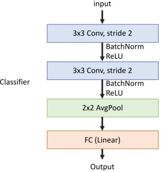
3.2.2 Classifier modification

After we change the input image to 1/4, most of the blocks in MSDNet can work normally, and the original feature map output will become 1/4. But in the Classifier after each block, because its structure includes Fully Connected Layer, there is a limit to the input data, so the Classifier structure needs to be modified. The architecture of the Classifier is shown in Figure 10. We believe that the image has retained more important features when pre-processing reduces the image by 1/4. Therefore, the feature values

(30)

should be retained at the end, and the feature value should not be reduced through AvgPool, so we chose to delete the AvgPool layer instead of adjusting the input of the Fully Connected Layer.

Figure 10: Classifier architecture in MSDNet 3x3 Conv, stride 2

input

Output 3x3 Conv, stride 2

BatchNorm ReLU BatchNorm ReLU

2x2 AvgPool

FC (Linear)

Classifier Classifier

(31)

Chapter 4 Experimental

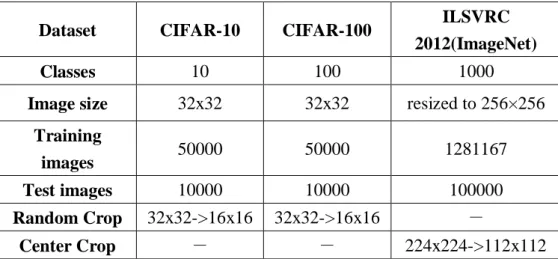
4.1 Dataset

In the experiment, we used the CIFAR-10, CIFAR-100 [9], and ILSVRC 2012 [10]

datasets. The detailed data of the dataset is shown in Table 2. In addition, the data- augmentation techniques used in our dataset are the same as the [1] paper to follow [12], including the following steps:

Step 1: zero-padded with 4 pixels, and then random cropped or center cropped images

（see table 2 for crop size）

Step 2: flipped horizontally（probability 0.5）

Step 3: to Tensor（If you are using Pytorch）

Step 4: normalized （according to the following formula）

𝐼𝑛𝑝𝑢𝑡[𝑐ℎ𝑎𝑛𝑛𝑒𝑙] =(𝐼𝑛𝑝𝑢𝑡[𝑐ℎ𝑎𝑛𝑛𝑒𝑙] − 𝑚𝑒𝑎𝑛[𝑐ℎ𝑎𝑛𝑛𝑒𝑙]) 𝑠𝑡𝑑[𝑐ℎ𝑎𝑛𝑛𝑒𝑙]

In Dataloader, it is assumed that 32 * 32 RandomCrop with padding 4 will be used for the image, but if our image is reduced to 1/4, the size of RandomCrop with padding 4 will

(32)

be modified to 16 * 16. In our method, if we use Wavelet transform and Resize, we need to make this modification. VAE and Mini NN do not need to be modified, they only need to modify the network architecture as in 3.2. But on the implementation, because VAE does not train with MSDNet, in order to speed up the overall training speed, we save the VAE Encoder results as image files to reduce the time of each repeated calculation.

Dataset CIFAR-10 CIFAR-100 ILSVRC

2012(ImageNet)

Classes 10 100 1000

Image size 32x32 32x32 resized to 256×256 Training

images 50000 50000 1281167

Test images 10000 10000 100000

Random Crop 32x32->16x16 32x32->16x16 －

Center Crop －－ 224x224->112x112

Table 2: Details of the experimental dataset

(33)

4.2 Training Details

We use the Pytorch version of MSDNet to do all the experiments. The parameters are set as shown in Table 3. Base represents the horizontal depth of the first block, and Step represents the horizontal depth of the other blocks. Most of parameters are based on the [1] paper settings, but the Batch Size is limited by our hardware, so we set the Batch Size 128 when we use ILSVRC 2012 (ImageNet) dataset.

Dataset CIFAR- 10

CIFAR- 100

ILSVRC 2012 (ImageNet)

Batch Size 64 64 128

Epoch 300 300 90

Block 10 7 5

Step 2 3 7

Base 4 4 7

Loss Function CrossEntropyLoss Optimizer

Stochastic Gradient Descent(SGD) momentum : 0.9

weight_decay : 0.1 Learning Rate

Epoch 0~149 : 0.1 Epoch 150~224 : 0.01

Epoch 225~ : 0.001

Epoch 0~29 : 0.1 Epoch 30~59 : 0.01

Epoch 60~ : 0.001 Table 3: Training parameter settings

(34)

4.3 Training Results

We will test on the three datasets of CIFAR-10, CIFAR-100, and ILSVRC 2012 (ImageNet) according to our proposed method and present the results below.

4.3.1 CIFAR-10 Results

Table 4 presents the accuracy of the CIFAR-10 dataset after training, where each value represents the accuracy output on a certain block, the red mark is the highest accuracy of the method, and the rightmost one shows the difference between the maximum accuracy (red mark) and the original accuracy. We can find that if the Conv3 method is used, the accuracy only loses 1.98%, and the results using the Mini NN method also lose about 2%. If you simply compare the accuracy of each block, some blocks can even have smaller differences in accuracy. In addition, we also observed that for the network architecture of the CIFAR-10 dataset, not all methods have the best results in the last block. We may think that some network architectures are too deep for this dataset, which will lead to a decrease in accuracy. If it is actually applied to an edge device, we can just use the block with the highest accuracy, so that we can save some computing resources spent on the block.

(35)

Table 4: The accuracy of CIFAR-10 after training

Table 5 presents the number of FLOPs required for each block prediction, and the values in parentheses show the ratio of FLOPs required compared to the original method.

The red mark in Table 5 is the FLOPs required by the block with the highest accuracy in this method. We also converted the percentage of FLOPs in Table 5 (compared with the original method) into Figure 11, so that we can better observe. We can see that the two methods Conv3 and Conv3 with shortcut require relatively high FLOPs at the beginning, and even exceed the original method, but the more blocks are calculated, the more FLOPs are reduced. Even the last block only requires 35% of FLOPs from the original method, which reduces the FLOPs by 65%. This phenomenon occurs because the network architecture in the two methods of Conv3 and Conv3 with shortcut uses more kernels to retain the image features. In addition, we also observed that the FLOPs of the VAE network are too large, resulting in the overall FLOPs far exceeding the original method,

Method \ Accuracy block1 block2 block3 block4 block5 block6 block7 block8 block9 block10 Max Accuracy Diff

Original 87.21 88.51 89.31 90.28 90.69 90.83 90.97 91.29 91.15 91.26 -

Conv3 86.16 87.19 88.11 88.7 88.83 88.88 89.31 88.99 89.1 89.13 -1.98

Conv3 with shortcut 86.07 87.16 88.18 88.26 88.82 88.82 89.26 88.91 88.87 89.01 -2.03

Conv2 85.41 86.63 87.25 88.08 88.53 88.64 88.82 88.71 88.79 89.09 -2.2

Conv1 83.41 85.75 87.08 87.75 88.52 88.61 89.07 88.67 88.65 88.45 -2.22

resize.CUBIC 77.17 81.52 82.63 83.54 84.06 84.3 84.47 84.8 84.72 84.79 -6.49

resize.AREA 77.22 80.63 82.04 83.47 83.47 84.15 84.03 84.54 84.46 84.5 -6.75

Maxpool 78.77 80.98 82.13 83.47 83.57 83.88 84.02 83.87 83.75 84.44 -6.85

resize.LINEAR 78.53 80.74 81.97 82.74 83.5 83.98 83.99 84.21 84.25 84.3 -6.99

resize.LANCZOS4 78.09 80.07 81.55 82.65 83.21 83.55 83.59 84.15 84.13 84.12 -7.14

resize.NEAREST 77.52 79.71 80.54 81.91 81.99 82.49 82.77 83.48 83.27 83.27 -7.81

wavelet(LL).MinMaxScaler 73.22 75.81 77.1 78.55 78.73 79.15 79.67 79.43 79.44 79.49 -11.62

wavelet(LL+HL+LH+HH) 70.46 73.1 74.64 76.86 77.87 78.35 78.65 78.78 78.88 78.76 -12.41

wavelet(LL+HL+LH) 72.32 73.99 75.48 76.83 77.27 77.61 78.18 78.46 78.49 78.49 -12.8

wavelet(LL) 72 74.33 75.56 77.14 77.61 77.84 78.01 78.27 78.24 78.34 -12.95

VAE 34.2 34.2 37.08 39.23 40.3 40.73 40.91 40.69 40.55 40.59 -50.38

(36)

so we can know that this method is not suitable for edge devices. Finally, we can see that the part of the red mark in Table 5 is the block with the highest accuracy in each method.

If we compare the cost of FLOPs with the highest accuracy block, the original method is 101M FLOPs, the three methods of Conv3, Conv3 with shortcut and Conv2 are about 35M FLOPs, which are about 65% less FLOPs than the original method, Conv1 cost 23.6M FLOPs reduced FLOPs about 76%, Maxpool cost 31M reduced about 69% FLOPs.

Table 5: FLOPs required for each block prediction in CIFAR-10

Figure 11:The percentage of FLOP required for each block prediction in CIFAR-10 relative to the original method

Method \ FLOPs(10^6) block1 block2 block3 block4 block5 block6 block7 block8 block9 block10 Original 16(100%) 26(100%) 38(100%) 53(100%) 64(100%) 76(100%) 89(100%) 101(100%) 111(100%) 123(100%) Conv3 16.3(102%) 19.3(74%) 22.3(59%) 26.3(50%) 28.3(44%) 31.3(41%) 35.3(40%) 38.3(38%) 40.3(36%) 43.3(35%) Conv3 with shortcut 16.4(103%) 19.4(75%) 22.4(59%) 26.4(50%) 28.4(44%) 31.4(41%) 35.4(40%) 38.4(38%) 40.4(36%) 43.4(35%) Conv2 6.8(43%) 9.8(38%) 12.8(34%) 16.8(32%) 18.8(29%) 21.8(29%) 25.8(29%) 28.8(29%) 30.8(28%) 33.8(27%) Conv1 4.6(29%) 7.6(29%) 10.6(28%) 14.6(28%) 16.6(26%) 19.6(26%) 23.6(27%) 26.6(26%) 28.6(26%) 31.6(26%)

Maxpool 4(25%) 7(27%) 10(26%) 14(26%) 16(25%) 19(25%) 23(26%) 26(26%) 28(25%) 31(25%)

VAE 334(2088%) 337(1296%) 340(895%) 344(649%) 346(541%) 349(459%) 353(397%) 356(352%) 358(323%) 361(293%) resize, wavelet 4(25%) 7(27%) 10(26%) 14(26%) 16(25%) 19(25%) 23(26%) 26(26%) 28(25%) 31(25%)

(37)

We compare the accuracy of Mini NN's experimental results with FLOPs in Figure 12, and we can see that the FLOPs used in our method are lower than the original ones. If the original method is used on an edge device with low computing resources, there may be no way to predict the first block. If we use our method, there may be at least a few block predictions results. In the edge device with the lower calculation capacity, it is recommended to use Conv1 or Conv2, because they have lower requirements for the FLOPs required for the first block, which can improve the reliability of the output prediction results of the edge device. Unless we have stable computing resources that can reach the first block of Conv3 or Conv3 with shortcut, in this case, it is recommended to use Conv3 or Conv3 with shortcut.

(38)

4.3.2 CIFAR-100 Results

In the same way that the results of the CIFAR-10 dataset are presented, we present the accuracy of the CIFAR-100 dataset after training using various methods in Table 6.

Among them, we can see that the highest accuracy (red mark) is mostly concentrated in the last block, which means that 7 blocks are not too deep for the CIFAR-100 dataset. In addition, in terms of accuracy, the minimum difference between the highest accuracy of the original method and other methods is 2.88%, and the accuracy difference in other blocks may be smaller. In particular, the accuracy of block1 in Conv3 and Conv3 with shortcut methods is better than the original method. Here we compare the FLOPs in Table 7 and find that the cost of FLOPs is higher than the original method, so this part maybe because of Conv3 and Conv3 with shortcut use more kernel extraction features in front, so it can get a higher accuracy.

Table 6: The accuracy of CIFAR-100 after training

Method \ Accuracy block1 block2 block3 block4 block5 block6 block7 Max Accuracy Diff

Original 58.18 62.62 65.96 66.77 67.75 67.92 68.67 -

Conv3 58.85 60.68 62.12 64.48 64.63 65.58 65.79 -2.88

Conv3 with shortcut 58.44 61.01 62.52 64.24 64.66 65.09 65.53 -3.14

Conv1 54.55 59.27 61.23 63.35 64.3 64.68 65.21 -3.46

Conv2 57 60.25 61.71 63.86 64.82 64.76 65.16 -3.51

resize.LINEAR 46.55 52.22 55.74 56.97 58.37 59.09 59.4 -9.27

resize.AREA 47.74 51.99 55.36 56.87 58 58.86 59.19 -9.48

Maxpool 50.2 54.55 55.64 57.4 58.6 58.88 58.69 -9.79

resize.CUBIC 47.36 51.4 55.25 56.92 57.83 58.35 58.6 -10.07

resize.LANCZOS4 47.48 51.56 55.16 56.82 57.56 58.22 58.34 -10.33

resize.NEAREST 46.61 50.78 55.06 55.9 57.76 57.49 57.84 -10.83

wavelet(LL).MinMaxScaler 41.25 44.67 48.4 49.87 50.74 51.03 51.71 -16.96

wavelet(LL+HL+LH) 39.05 42.08 45.65 46.82 48.17 49.23 49.25 -19.42

wavelet(LL) 40.22 43.48 46.89 48.07 48.84 49.17 49.23 -19.44

wavelet(LL+HL+LH+HH) 39.1 43.1 45.73 46.81 48.39 49.07 48.64 -19.6

VAE 14.48 16.1 18.65 19.72 19.34 19.66 19.99 -48.68

(39)

Table 7 shows the number of FLOPs required for each block prediction in the CIFAR- 100 dataset. Figure 13 shows the percentage of FLOPs required for each block prediction compared with the original method. The presentation method is the same as that of the CIFAR-10 data set, and the result is similar to the CIFAR-10 dataset. We can reduce FLOPs by at least 64%, but the accuracy can be maintained at a loss of about 3%. If we compare the cost of FLOPs with the highest accuracy block, the original method costs 109M FLOPs, Conv3 and Conv3 with shortcut cost about 39M FLOPs, which reduces FLOPs by about 64%, and Conv1 costs 28M FLOPs, which reduces FLOPs by about 74%. , Conv2 cost 30M FLOPs, which reduced FLOPs by about 72%, Maxpool costs 24M FLOPs, which reduced FLOPs by about 78%.

Table 7: FLOPs required for each block prediction in CIFAR-100

Method \ FLOPs(10^6) block1 block2 block3 block4 block5 block6 block7

Original 16(100%) 30(100%) 48(100%) 62(100%) 79(100%) 95(100%) 109(100%) Conv3 16.3(102%) 19.3(64%) 24.3(51%) 27.3(44%) 32.3(41%) 36.3(38%) 39.3(36%) Conv3 with shortcut 16.4(103%) 19.4(65%) 24.4(51%) 27.4(44%) 32.4(41%) 36.4(38%) 39.4(36%) Conv1 4.6(29%) 7.6(25%) 12.6(26%) 15.6(25%) 20.6(26%) 24.6(26%) 27.6(25%) Conv2 6.8(43%) 9.8(33%) 14.8(31%) 17.8(29%) 22.8(29%) 26.8(28%) 29.8(27%)

Maxpool 4(25%) 7(23%) 12(25%) 15(24%) 20(25%) 24(25%) 27(25%)

VAE 334(2088%) 337(1123%) 342(713%) 345(556%) 350(443%) 354(373%) 357(328%) resize, wavelet 4(25%) 7(23%) 12(25%) 15(24%) 20(25%) 24(25%) 27(25%)

(40)

Figure 13: The percentage of FLOP required for each block prediction in CIFAR-100 relative to the original method

We also show the comparison of Mini NN's accuracy and FLOPs in Figure 14, and the trend shown in the figure is similar to the results of the CIFAR-10 dataset. The FLOPs used in our method are lower than the original method. What is special in the CIFAR-100 dataset is that the result of the last block of Conv1 is a little better than the result of the last block of Conv2, but the results of other Conv1 blocks are not better than Conv2, so in the selection method, we recommend to confirm that whether the edge device can always predict the last block, and then choose Conv1 or Conv2 method. It can be seen from the above situation that the accuracy of Mini NN's method is not much different, so on edge devices with limited resources, we should choose the method to use according to the energy and application characteristics of the device.

(41)

Figure 14: CIFAR-100 dataset experiment results

(42)

4.3.3 ILSVRC 2012 (ImageNet) Results

In the same way that the results of the CIFAR-10 dataset are presented, we present the accuracy of the ImageNet dataset after training using various methods in Table 8. The same phenomenon as the CIFAR-100 dataset, the highest accuracy(red mark) in the table is mostly concentrated in the last block, which means that 5 blocks are not too deep for the ImageNet dataset. Besides, in terms of accuracy, the minimum difference between the highest accuracy of the original method and other methods is 2.45%. The difference between this part and other datasets is that the accuracy of the last block of resize.LINEAR is a little higher than Conv1, but the accuracy of other blocks is still lower than Conv1, so if the edge device can predict the result steadily until the last block, choose to use resize.LINEAR method will be better.

Table 8: The accuracy of ImageNet after training

Method \ Accuracy block1 block2 block3 block4 block5 Max Accuracy Diff

Original 62.924 69.864 73.178 73.728 74.672 -

Conv3 60.146 67.864 70.89 71.538 72.222 -2.45

Conv3 with shortcut 60.942 67.602 70.13 70.45 71.094 -3.578

Conv2 59.632 67.292 69.914 70.176 71.012 -3.66

resize.LINEAR 55.604 63.468 66.92 67.714 68.776 -5.896

Conv1 57.298 65.354 67.074 67.836 68.462 -6.21

resize.LANCZOS4 54.506 62.152 66.134 67.328 68.166 -6.506

resize.CUBIC 54.706 62.642 65.998 66.676 67.592 -7.08

Maxpool 54.768 63.046 65.588 65.948 66.984 -7.688

resize.NEAREST 53.98 62.448 65.414 65.926 66.948 -7.724

resize.AREA 55.01 62.588 64.992 65.516 66.31 -8.362

(43)

Table 9 presents the number of FLOPs required for each block prediction in the ImageNet dataset. Figure 15 shows the percentage of FLOPs required for each block prediction compared with the original method. The presentation method is the same as that of the CIFAR-10 dataset. We can reduce FLOPs by at least 50%, but the accuracy can be maintained at a loss of about 2.5%. If we compare the cost of FLOPs with the highest accuracy block, the original method costs 3.2GFLOPs, Conv3 and Conv3 with shortcut cost about 1.6G FLOPs, which reduces the FLOPs by 50%, Conv1 costs 0.9G FLOPs, which reduces FLOPs by about 72%, Conv2 costs 1G FLOPs, which reduces FLOPs by about 67%, and Maxpool costs 0.8G FLOPs, reduced FLOPs by about 74%.

Table 9: FLOPs required for each block prediction in ImageNet

Figure 15: The percentage of FLOP required for each block prediction in ImageNet

Method \ FLOPs(10^9) block1 block2 block3 block4 block5

Original 0.621(100%) 1.445(100%) 2.294(100%) 2.98(100%) 3.267(100%)

Conv3 0.954(154%) 1.165(81%) 1.384(60%) 1.562(52%) 1.643(50%)

Conv3 with shortcut 0.957(154%) 1.169(81%) 1.388(60%) 1.566(53%) 1.647(50%)

Conv2 0.386(62%) 0.597(41%) 0.816(36%) 0.994(33%) 1.075(33%)

Conv1 0.23(37%) 0.441(31%) 0.669(29%) 0.838(28%) 0.919(28%)

Maxpool 0.16(26%) 0.371(26%) 0.59(26%) 0.768(26%) 0.849(26%)

resize, wavelet 0.16(26%) 0.371(26%) 0.59(26%) 0.768(26%) 0.849(26%)

(44)

We present the comparison of accuracy and FLOPs in Figure 16, and the trends presented in the figure are similar to the CIFAR-10 and CIFAR-100 datasets, and our methods cost less FLOPs than the original method. We found that Conv3 has only 60%

accuracy at 1G FLOPs, but Conv2 is as high as 70%, and the original method is about 63%, so we think Conv3 costs too many FLOPs. Therefore, it is recommended that in a larger network architecture, if the edge device does not have stable calculation capacity, the Conv3 method is not recommended. In the choice of other methods, we recommend choosing Conv2 first, because it requires less FLOPs and higher accuracy. If the calculation capacity of the edge device cannot be achieved, we recommend the Conv1 or the resize.LINEAR method.

(45)

According to the experimental results of the three datasets, we can observe that the accuracy of Mini NN is higher than other methods. We think that because Mini NN will train with MSDNet, so Mini NN method can produce a better kernel through training to retain important features. Compared with the methods of Resize and Wavelet transform, there is no way to extract customized features for the dataset, so there is no way to retain more important features. For the VAE part, although the features that can be decoded into the original image are extracted through training, but this feature may not be suitable for classification, so the final result is not good. For the use of edge devices, we recommend the Mini NN method. In addition to the Maxpool method in Mini NN, other Mini NN methods can be selected and used according to the characteristics of the device. If the computing resources are unstable or need real-time applications, you can choose the Conv1 method, because the FLOPs required in the first block prediction will be the smallest, increasing the probability of outputting the prediction results and shortening the prediction latency. If the computing resources are relatively stable, but there is often no way to predict the last block, it is recommended to use Conv2, this method can have a higher accuracy, and the FLOPs required for the first block output need not be too large, and the latency of prediction is not too long. If the edge device can calculate the last block every time, it is recommended to use Conv3. This method greatly reduces FLOPs

(46)

compared to the original method but can maintain a certain accuracy, suitable for use in edge devices with lower calculation capacity.

(47)

Chapter 5 Conclusions and Future Works

In this thesis, we have proposed methods for processing network input, including CNN, VAE, Resize, and Wavelet transform, to reduce the large number of FLOPs cost by the neural network, so that the neural network can be smoothly used on edge devices with lower calculation capacity. It can also meet the real-time application of edge devices and allow edge devices with limited resources to have reliable prediction results. We use CIFAR-10, CIFAR-100, ILSVRC three datasets to do related experiments, analyze and compare our proposed methods, and discuss the methods applicable to edge devices, and finally give relevant suggestions. In general, the method using Mini NN can achieve better results on edge devices, reduce more FLOPs, and lose less accuracy than other methods.

In future work, we hope that we can achieve higher accuracy by modifying the Mini NN or the network itself. We also hope to modify the MSDNet architecture so that the FLOPs cost between each block can be further reduced. Finally, we hope to apply these methods outside of MSDNet, expect to achieve similar results or find out why they cannot be used, and propose better methods in the further.

(48)

References

[1] Gao Huang, Danlu Chen, Tianhong Li, Felix Wu, Laurens van der Maaten,and Kilian Weinberger, “Multi-scale dense networks for resource efficient image classification,” in International Conference on Learning Representations, 2018.

[2] M. Bojarski, D. D. Testa, D. Dworakowski, B. Firner, B. Flepp, P. Goyal, L. D.

Jackel, M. Monfort, U. Muller, J. Zhang, X. Zhang, J. Zhao, and K. Zieba, “End to end learning for self-driving cars,” CoRR, 2016.

[3] C. Chen, A. Seff, A. Kornhauser and J. Xiao, “DeepDriving: Learning Affordance for Direct Perception in Autonomous Driving,” 2015 IEEE International Conference on Computer Vision (ICCV), Santiago, 2015, pp. 2722-2730, doi:

10.1109/ICCV.2015.312.

[4] Y. Deng, A. Luo and M. Dai, “Building an Automatic Defect Verification System Using Deep Neural Network for PCB Defect Classification,” 2018 4th International Conference on Frontiers of Signal Processing (ICFSP), Poitiers, 2018, pp. 145-149, doi: 10.1109/ICFSP.2018.8552045.

[5] A. Esteva et al., “Dermatologist-level classification of skin cancer with deep neural networks,” Nature, vol. 542, no. 7639, pp. 115–118, 2017.

[6] D. Silver, J. Schrittwieser, K. Simonyan, I. Antonoglou, A. Huang, A. Guez, T.

(49)

Hubert, L. Baker, M. Lai, A. Bolton et al., “Mastering the game of go without human knowledge,” Nature, vol. 550, no. 7676, pp. 354-359, Oct. 2017.

[7] D. P. Kingma and M. Welling, “Auto-encoding variational Bayes,” in Proc. Int. Conf.

Learn. Representations (ICLR), 2014.

[8] C. Doersch, “Tutorial on variational autoencoders,” 2016, arXiv:1606.05908.

[Online]. Available: http://arxiv.org/abs/1606.05908

[9] A. Krizhevsky and G. Hinton, “Learning multiple layers of features from tiny images,” Dept. Comput. Sci., Univ. Toronto, Toronto, ON, Canada, Tech. Rep., 2009. [Online]. Available: https://www.cs.toronto.edu/~kriz/learning-features-2009- TR.pdf

[10] J. Deng, W. Dong, R. Socher, L. Li, Kai Li and Li Fei-Fei, “ImageNet: A large-scale hierarchical image database,” 2009 IEEE Conference on Computer Vision and Pattern Recognition, Miami, FL, 2009, pp. 248-255, doi:

10.1109/CVPR.2009.5206848.

[11] C. Szegedy et al., “Going deeper with convolutions,” 2015 IEEE Conference on Computer Vision and Pattern Recognition (CVPR), Boston, MA, 2015, pp. 1-9, doi:

10.1109/CVPR.2015.7298594.

[12] K. He, X. Zhang, S. Ren and J. Sun, “Deep Residual Learning for Image Recognition,” 2016 IEEE Conference on Computer Vision and Pattern Recognition