國立臺灣大學生物資源暨農學院昆蟲學系 碩士論文
Department of Entomology
College of Bioresources and Agriculture National Taiwan University
Master Thesis
熱帶火蟻之性別決定機制探討
What type of sex determination does Solenopsis
geminata use?
A focus on the homologous SDL region
陳沐恩 Mu-En Chen
指導教授:王忠信 博士 黃榮南 博士 Advisor: John Wang, Ph.D.
Rong-Nan Huang, Ph.D.
中華民國 106 年 1 月
I
國立臺灣大學(碩)博士學位論文
口試委員會審定書
熱帶火蟻之性別決定機制探討
What type of sex determination does Solenopsis geminata use?
本論文係陳沐恩君(R03632006)在國立臺灣大學昆蟲學 系、所完成之碩士學位論文,於民國 106 年 1 月 13 日承下列 考試委員審查通過及口試及格,特此證明
口試委員:
(指導教授) (指導教授)
系主任
doi:10.6342/NTU201703365
致謝
事實上,這篇論文的完成讓我百感交集。從小我對於大自然的各樣事物就充滿了熱 情,希望可以知道更多一點。但不幸的是,”興趣大於能力” 也同時一直是我身 上的標籤。這樣的情況持續到我碩士班第一年,甚至一度在實驗室待不下去。但感 謝上帝,在這裡相遇相處的人們都或多或少的幫助著我,無論是我最廢最無貢獻的 時候還是我近期比較有 ”產出” 的時候我都可以感受到大家的溫暖與支持。謝 謝楊景程學長與我分享關於螞蟻獨特的一切,而且更重要的是若沒有約六年前您 的邀約,我現在完全不可能在這個實驗室裡,進行這些研究。感謝李志琦學長與黃 裕清學長,謝謝您們與我一起發想討論,無論是當時有用的沒用的都是很棒的啟發,
尤其您們分享的很多關於入侵紅火蟻的資料讓我可以一一比對並尋找適合我的研 究的方法,這幾乎是這篇論文的根基。謝謝張家寧(Tiffany)學姐、高嘉宜學姊、
蕭丞凱學長、鄧小美(Viet Dai Dang)學姐、丘祐坤學長,謝謝您們與我分享很多 技術相關的事務,完成這篇論文您們真的幫助很大。謝謝張倪禎、羅韻華、許蓉禎、
楊昉蓉、方森雅(Silvia Fontana),您們的鼓勵、支持與與日常的垃圾話(其實想 一想這些真的很有幫助)給了我很多繼續下去的動力。謝謝我的好同學張少濬還有 林羿岑,你們給了我很多很實際的幫助,讓我不至於因為實驗室不在學校而與世隔 絕。當然,真的非常感謝黃榮南老師願意收留我以及 John 的耐心指導,沒有您們 我現在絕對不是如此。最後,感謝我的家人接納我壓力很大的壞脾氣以及持續的支 持我。當然,感謝我的上帝一路的帶領,這篇論文為您而發。謝謝大家。
中文摘要
對於有性生殖之生物而言,性別決定是非常重要的。多數昆蟲性別決定機制之下游 部分是相當保守,但上游基因卻不然。入侵紅火蟻(Solenopsis invicta) 是使用單基 因座互補性別決定機制 (single-locus complementary sex determination, sl-CSD) 的 真社會性膜翅目昆蟲。 因此,異型合子 (heterozygosity) 個體將發育成雌性,但 半型合子 (hemizygosity) 或同型合子 (homozygosity) 個體則會發育為雄性。 我 們實驗室過去的研究顯示入侵紅火蟻決定性別基因有別於已被深入研究之另一真 社會昆蟲蜜蜂 (Apis mellifera),我們將其命名為 sex determination locus (SDL)。 即 便 目 前 尚 未 得 到 此 基 因 之 序 列 , 此 基 因 已 被 證 實 位 於 一 高 度 變 異 區 域 (hypervariable region)。本研究欲確認另一同屬的螞蟻:熱帶火蟻 (Solenopsis geminata)是否亦是使用此新發現之性別決定基因,但由於目前為止尚未有雙套體
雄蟲之紀錄,因此本研究將測試雌性個體是否全為異型合子。本研究記錄了與入侵 紅火蟻 hypervariable region 同源區域附近的 10 個微衛星 (microsatellite) 基因座 之基因型,並檢定其是否如同 CSD 機制一樣偏離哈溫平衡 (Hardy-Weinberg
equilibrium),結果顯示並未有顯著不同,後續的模擬資料顯示這是由於樣本數不 足而造成。因此,這些微衛星資料被組成單倍群 (haplotype), 並確認是否有任一 區域是如同 CSD 機制預期之雌性個體均為異型合子,合乎預期之位置在一橫跨連 續五個基因座的區域內被找到,且與隨機得到相同結果的機率有顯著不同。另外,
我們亦比較了 hypervariable region 序列在此兩種火蟻間的區別。系統發生樹
(phylogenic tree) 顯示在此區域有跨種多型性 (trans-species polymorphism) 之現 象,而在平衡選汰 (balancing selection) 下此為一常見之模式。 CSD 機制必然與 平衡選汰相關,因此綜合上述證據,我們可以間接了解此兩種全球入侵性螞蟻,即 便分別已久,SDL 同源區域仍在其性別決定機制中扮演著重要的角色。
關鍵字:性別決定機制、入侵紅火蟻、熱帶火蟻、平衡選汰、跨種多型性
Abstract
Sex determination is absolutely critical for sexual organisms. For most insect species the downstream components of the sex determination pathway are conserved, but the upstream genes and mechanisms are very diverse. The red imported fire ant (Solenopsis invicta, RIFA) is a eusocial Hymenoptera which uses the single-locus complementary sex
determination (sl-CSD) mechanism whereby heterozygosity at a single sex locus results in females and hemizygosity (or homozygosity) at this locus yields males. Our lab has shown that the master trigger gene for RIFA sex determination, sex determination locus (SDL), is different from that of the honey bee (Apis mellifera). Although SDL has not been cloned in RIFA, it is characterized by a hypervariable region. I tested whether the tropical fire ant (Solenopsis geminata, TFA) also uses SDL, which I hypothesize is likely because these two species are congeneric. Conservation of function between these two species predicts that TFA SDL will always be heterozygous in females and homozygous in males. Diploid males were not available so this study focused on females.
I genotyped 10 microsatellite loci in TFA that are putatively orthologous to RIFA loci near the hypervariable region. Absolute female heterozygosity would violate Hardy-Weinberg equilibrium, but analysis of these microsatellite data could not rejected the Hardy- Weinberg model, likely because of insufficient power given the large number of sex alleles. Nevertheless, by constructing 5-loci haplotypes, I never found any homozygous
haplotypes in females, consistent with the CSD model. In addition, the phylogenic tree of the hypervariable region and the nearby gene EGF-like revealed trans-species polymorphisms between TFA and RIFA indicating that the alleles may be older than these two species and suggesting that SDL is likely evolving under balancing selection.
Together my results indicate that the homologous SDL locus could be important for sex determination in S. geminata.
Keywords: sex determination, fire ant, Solenopsis invicta, Solenopsis geminata, balancing selection, trans-species polymorphism
Table of Contents
口試委員會審定書………..………….………I
誌謝……….……….……II
中文摘要……….…III Abstract………...…..V Table of contents………VII List of Figures………..………...X List of Tables………...XI Abbreviation Table ……….………...XII
1. Introduction………..………1
1.1 Sex determination systems……….………...1
1.2 Core sex determination genes are conserved………..………2
1.3 Honeybees and the red imported fire ants (RIFA)………….……….3
1.4 Tropical fire ant (Solenopsis geminata Fabricius, TFA)……..…...4
1.5 Key questions and the hypothesis…..……….…….5
1.6 General research strategy………….………..6
2. Materials and methods ………...…9
2.1 Sample collection………..………9
2.2 Ant husbandry………9
2.3 Microsatellite data analysis……….…………....10
2.3.1 The reference genome………...………… 10
2.3.2 Primer design………...…… 10
2.3.3 DNA extraction……….……….………...11
2.3.4 Multiplex PCR………....………...11
2.3.5 Capillary electrophoresis and microsatellite allele identification…...12
2.3.6 Hardy-Weinberg test………..……….12
2.3.7 Simulation data for the Hardy-Weinburg test………..…...13
2.3.8 The determination of phased data and heterozygosity power analysis....14
2.4 SDL homologous sequence analysis………..………15
2.4.1 The homologous sequences of RIFA and outgroup species………....15
2.4.2 DNA extraction……….…..….………....16
2.4.3 Primer design………..………....16
2.4.4 Selection of candidate neutral loci……….………..16
2.4.5 Cloning and sequencing………..………...17
2.4.5.1 Specific fragment PCR………...………...…17
2.4.5.2 Transformation, culturing, and sequencing……...…………...18
2.4.6 Analysis of nucleotide diversity and molecular evolution……...…18
3. Results………20
3.1 Microsatellite data and the Hardy-Weinburg test potentially suggest that the homologous hypervariable region could function in TFA sex determination...20
3.1.1 Sequence data show that the SDL homologous region of TFA is similar to RIFA's………..20
3.1.2 Hardy-Weinberg equilibrium model could not be rejected based on single microsatellite locus analysis………..………...…20
3.1.3 The exact simulation p-value indicates that a sample size of 1.3 times the allele number is necessary to make the analysis significant…...…21
3.1.4 Analysis of heterozygosity of haplotype blocks potentially suggest that the region between THUMP to SDL6-4 as the candidate SDL locus...…21
3.2 Balancing selection is supported in the homologous sequence in the hypervariable region.……….22
3.2.1 The description of the hypervariable region and the nearby region and
genes……….…...22
3.2.2 Gene tree analyses support trans-species polymorphism (TSP) in the hypervariable region ……….………… ………...23
4. Discussion……….26
4.1 Structural similarity between TFA and RIFA at the SDL homology candidate region……….………..…………..……..26
4.2 Information from single microsatellite markers are insufficient to confirm or refute the sex locus……….………...26
4.3 The highly diverse haplotypes at the SDL region in TFA……….27
4.4 Balancing selection could be supported by the TSP phenomenon………...…28
5. References………..45
Appendix………..……….50
List of Figures
Figure 1. Comparison of the candidate sex locus within the SDL region of TFA and
R IFA. ………..……….. ..30
Figure 2. Hardy-Weinberg simulation analysis. ……….…....31
Figure 3. The hypervariable and surrounding region. ………....32
Figure 4. The shared “insertion” between TFA and RIFA. ………....33
Figure 5. Phylogenic trees of the hypervariable and surrounding regions. ………....34
Figure 6. Phylogenic trees of the neutral regions. ………..……….…....38
List of tables
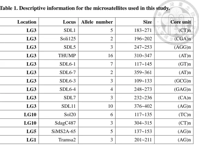
Table 1. Descriptive information for the microsatellites used in this study.………….41 Table 2. Summary of the Hardy-Weinberg analysis of diploid female microsatellite data.……….42 Table 3. Haplotype patterns for all 3, 4, or 5 adjacent loci combinations in the focal sex locus region………..………43 Table 4. The average nucleotide divergence (per site) within and between RIFA and TFA………… ……… ……… … … ……… ….44
Abbreviation Table
Abbreviation Full name
Blastn Basic Local Alignment Search Tool
CSD Complementary Sex Determination INDEL Insertion and Deletion
MAFFT Multiple Alignment using Fast Fourier Transform progress PCR Polymerase Chain Reaction
QTL Quantitative Trait Locus RIFA Red Imported Fire Ant TFA Tropical Fire Ant
TSP Trans-Species Polymorphism
1. Introduction
Life on Earth can be divided into asexual and sexual organisms. Compared to the simpler self-replication of asexuality, sexual reproduction is more complex and energetically expensive. Despite these costs, there are some distinct advantages for sexual reproduction. First, sexual reproduction involves the combining and mixing of genetic traits through their gametes which permits faster evolution and adaptation. Second, sexual reproduction can purge the genome of deleterious mutations through meiotic recombination (Kondrashov, 1988; Muller, 1964) and thereby also increasing the fitness of a population.
In animals, males and females are often sexually dimorphic. Examples include the larger body size of female spiders or the horns of male goats. An individual’s sex is also associated with sex-specific behaviors. These sex-specific morphologies and behaviors often intersect through sexual selection. Thus, proper sex determination is absolutely critical for the fitness of sexual organisms.
1.1 Sex determination systems
Although some species employ environment -dependent sex determination (e.g., temperature-dependent sex determination), the majority of species use genetic sex determination mechanisms with the most familiar being the XY sex determination system. In this system, females are homozygous for one of the sex chromosomes, XX, and males are heterozygous, XY. This system is referred to as male heterogamety and includes humans and most vertebrates. Another kind of sex determination is female heterogamety, or the ZW sys tem, where females are heterozygous for the sex chromosomes, ZW, and males are homozygous, ZZ.
This second system is very common in avian and lepidopteran (butterflies and
moths) species. A third system, which is the focus of this study, is haplodiploid sex determination where females are diploid and males are haploid (Heimpel and de Boer, 2008). Wasps, honeybees, and ants employ this. Outside of the honeybee, the genetic and molecular mechanisms in hymenoptera are unclear.
1.2 Core sex determination genes are conserved
Even though there are many mechanisms to initiate the sex determination pathway, they all seem to converge on two components. The first is the splicing factor, transformer (tra), which causes sex-specific splicing of the second component, the transcription factor, doublesex (dsx). In contrast to these two genes, the master trigger genes and mechanisms are very diverse (Gempe and Beye, 2011). The fruit fly (Drosophila melonogaster) uses sex-lethal (sxl) to determine their sex (Bell et al., 1988). The housefly (Musca domestica) uses Musca domestica male determiner (Mdmd) to determine whether an individual will develop into a male (Sharma et al., 2017). The red flour beetle (Tribolium castaneum) and a wasp (Nasonia vitripennis) both have maternal control of their sex determination, although the maternally regulated genes are different (Beukeboom and Van De Zande, 2010; Shukla and Palli, 2012). Finally, honeybees (Apis mellifera) use the complementary sex determination (CSD) system via the eponymously named gene, csd (Beye et al., 2003).
The master trigger genes evolve relatively fast (Bachtrog et al., 2014). The housefly is a good example. In most housefly populations, the male-determining factor (M factor) is on the Y chromosome and inhibits the feminizing factor which is on the X chromosome. However, in other populations the M factor may be located on a former autosome or even on the prior X chromosome (Inoue et
al., 1983).
1.3 Honeybees and the red imported fire ants (RIFA)
Honeybees are haplodiploid organisms, and also are the most well understood hymenopteran system. The discovery of viable dipl oid males permitted the genetic dissection of the honeybee sex determination pathway.
They use the complementary sex determination system. In this mechanism, there are one or several loci that determine sex. The simplest case is single locus complementary sex determination (sl-CSD) where the individuals who are heterozygous at this locus develop into females. Individuals that are homozygous or hemizygous at this locus, develop into males (Ross, 1985). It is worth noting that diploid males are often sterile.
At the molecular level, when a honeybee individual is heterozygous at the master trigger gene, csd, the protein product of this gene causes female-specific splicing of the downstream gene feminizer (fem) (Gempe et al., 2009). Then the female-specific isoform of fem causes female-specific splicing of doublesex (dsx).
Note that fem is a homolog of the gene tra and csd is a paralog of the gene fem (Biewer et al., 2015). On the other hand, for individuals that are homozygous or hemizygous for csd, the csd protein product does not promote female-specific fem splicing; fem is spliced to the default male form. Consequently, dsx is also spliced as the male form. Thus like in other insects, the sex -specific isoforms of dsx, ultimately regulate proper sexual fate (Cho et al., 2007).
Although the honeybee and the red imported fire ant ( Solenopsis invicta Buren, RIFA) are both eusocial Hymenoptera and use the single -locus CSD mechanism, quantitative trait locus (QTL) analysis and genetic mapping
conducted in our lab has revealed that the RIFA sex locus of RIFA is not at the tra homologous region. Instead, the sex locus, which we call sex determination locus (SDL), is on a different chromosome (Huang et al., unpublished).
Hymenopteran species are no exception with respect to quickly evolving upstream sex determination genes. In addition to the fire ant case, allelic variability of the tra homolog or paralog is absent from the genome of bumblebee (Bombus terrestris and Bombus impatiens) that indicates they determine their sex by something else (Sadd et al., 2015). To understand the evolution of the master trigger gene for sex in the genus Solenopsis, the related tropical fire ant (Solenopsis geminata, TFA) is examined to determine whether it also uses SDL like RIFA or some other gene(s).
1.4 Tropical fire ant (Solenopsis geminata Fabricius, TFA)
TFA is an invasive species. Their native habitat is in Central America and northern South America. The current invasion model is that they spread throughout the world from the southwest of Mexico because of global commerce in the 16th century to Manila. After TFA moved from Manila to Taiwan, a nd then from Taiwan to many Old World tropical regions (Gotzek et al., 2015). In Taiwan, they are located in the southern, central (Lai et al., 2009), and eastern (Retrieved July 24, 2017, from http://taibif.tw/zh/namecode/341929) regions. They are a very common ant species currently and have even become agricultural pests.
Phylogenetically, both RIFA and TFA belong to the genus Solenopsis, but TFA is classified as a relatively basal species in the “fire ant” group based on morphology (Pitts et al., 2005) and the mitochondrial genome (Gotzek et al., 2010). Furthermore, the genome of RIFA is already available (Wurm et al., 2011),
and TFA was chosen to compare to the RIFA sex determination region because they are common in Taiwan and their genome is also ava ilable (C.C. Lee and J.
Wang, personal communication).
1.5 Key questions and the hypothesis
In this study, I used the two invasive ants, TFA and RIFA, to investigate the evolution of the master sex determination genes after speciation. Conservation or diversification of function at the orthologous sex locus between these two species will be informative of the rate of sex lo cus change in ants, at least for the Solenopsis clade. I hypothesized that TFA uses the orthologous SDL locus as RIFA for sex determination because of their phylogenetic relatedness. Other mechanisms are possible, and examples occur in Hymenoptera. For ins tance, sex determination may be multiple-locus CSD like some parasitic wasps (Snell, 1935) and the ant Vollenhovia emeryi (Miyakawa and Mikheyev, 2015). In another case, the master trigger gene may be epigenetically regulated such as in the jewel wasp Nasonia vitripennis (Verhulst et al., 2010).
In my hypothesis, we would expect to observe that all females are heterozygous at the SDL locus and diploid males are homozygous. In principle, the strongest evidence would come from diploid males. However, there are no reports of diploid males in TFA. This may be partly due to the fact that all reports of TFA in Taiwan are monogyne colonies (with only one queen) (Lai et al., 2009), which are unlikely to produce diploid males. In RIFA, newly “match -mated”
queens can survive in polygyne colonies but will fail to found independent monogyne colonies because the diploid males take too much of the resources from the first batch of workers (Ross and Fletcher, 1986). TFA is likely to be
similar to RIFA in this regard. Thus, obtaining diploid males is extremely unlikely at this time.
An alternative tactic is to test if the sex locus is always heterozygous in females. The risk of this method is that if there are many alleles at this locus, as predicted from theory for complementary sex determination, then the expected heterozygosity may already be high from simple random mating. Therefore, very large sample sizes may be necessary. Nevertheless, this is the method I have chosen because it is the only obtainable evidence.
1.6 General research strategy
I conducted three genetic analyses to test if the homologous SDL locus may function as the sex locus in TFA.
First, since the CSD mechanism implies that all heterozygous individuals develop into females, the prediction is that female data should not fit the Hardy - Weinberg equilibrium model. This test assumes an ideal population genetic model with infinite size and random mating as well as no mutation, migration, or selection. Since the genotypes of workers are identical to that of virgin queens (next generation queens), the analysis of worker genotypes should reflect the allele frequency of colonies in next generation. Therefore, I obtaine d microsatellite genotypes from many workers and conducted a Hardy-Weinberg equilibrium test of this basic population parameter.
Microsatellites are short tandem repeats in a genome that often have length polymorphism among individuals. Multiple loci can be composed into haplotypes.
We can quickly determine if a diploid individual is heterozygous or homozygous through this method. In addition, I collected additional information of unlinked
microsatellite loci as a control group for comparison. Analysis of single microsatellites could be problematic if the mutation rate of the microsatellite markers is much faster than for the SDL, resulting in some true homozygotes at SDL appearing falsely heterozygous. The use of multilocus haplotype markers can circumvent this issue. Thus, for the Hardy-Weinberg analyses, I constructed and examined microsatellite the haplotypes of the microsatellite loci that were tightly linked to SDL.
Second, Hardy-Weinberg equilibrium just tests for a reduction in female homozygosity, but actually the sex locus should never be homozygous. Direct inspection of the microsatellite haplotypes may be informative. Specifically, homozygous regions can be used to exclude sex locus regions. Conversely, invariably heterozygous regions would suggest candidate sex locus regions.
Third, the CSD sex locus should be under balancing selection because the fitness of heterozygotes is greater than homozygotes (heterozygote advantage) and lower frequency alleles have a selective advantage (negative frequen cy- dependent selection). Thus, selection would maintain or even increase multiple alleles over long evolutionary time (Garrigan et al., 2003); some alleles can become trans-species polymorphisms (TSP). TSP means that the allele sequences are more similar among species than within species (Klein, 1980). If three alternative possibilities, convergence (Andersson et al., 1991), introgression (Wegner and Eizaguirre, 2012), and new speciation (Nagl et al., 1998) could be excluded, TSP would be the strongest evidence for balancing selection (Takahata, 1990).
I examined the phylogenetic trees of the homologous regions whic h are tightly link to SDL. For controls, I also examined some neutral or independent
region. Finding evidence for balancing selection at the target region would indirectly support the hypothesis that TFA uses the same or similar sex determination mechanism with RIFA.
2. Materials and methods
2.1 Sample collection
Tropical fire ant colonies were collected in central and southern Taiwan between 2014 November to 2015 October. The locations were the eastern district of Tainan, Yunlin Dounan, Taichung Wurih, and Taichung Wuqi. Colonies and the surrounding dirt were dug out with a shovel and placed into buckets. Upon were returned to the lab, water was dripped into the buckets to slowly force ants to move to the surface.
Unlike S. invicta, in which workers and queens efficiently move into paper cups placed on top of the dirt, the queens of S. geminata are difficult to collect. Thus, we modified the standard fire ant protocol. Instead, a bridge was placed from the bucket to a plastic box (39 * 28 * 11 cm) containing an artificial nest. This allowed us to verify that the brood and queen had successfully moved into the artificial nest.
I also obtained some individual samples collected by friends. In total, 35 colonies were included in this study. Sample information is in appendix 1.
2.2 Ant husbandry
Colonies were housed in boxes with the inside walls coated with fluon to prevent ant escape. Occasionally, if the fluon was degraded and a new fluon-coated box was unavailable, baby powder would be applied to the rim of the box to temporarily prevent escape. Colonies were provided with 15 cm diameter petri dishes whose bottom were covered with plaster and to which water was added as needed to maintain humidity for shelter. Test tubes with water and plugged with cotton were also provided. All colonies were fed mealworms, crickets, and seeds 3 times per week. Temperature was maintained at 27⁰C to 30⁰C and the humidity was about 60%.
2.3 Microsatellite data analysis
2.3.1 The reference genome
The TFA reference genome was sequenced and assembled by our lab. There are three versions. The first version was assembled de novo from Illumina Solexa data (Bentley et al., 2008) derived from DNA extracted from a single TFA haploid male. The second one was assembled de novo from DNA extracted from a worker pool and sequenced using the PacBio Single Molecule, Real-Time (SMRT) Sequencing platform (Eid et al., 2009). This worker pool was from another colony and may include three different alleles. The last one was another assembly from the raw-data of the second version but with the potential alternate allele contigs included (C.C. Lee and J. Wang, personal communication). The third assembly is also the sequence which was analyzed, see below.
2.3.2 Primer design
In a RIFA study, 15 microsatellite primers were used to help map the sex determination locus (Huang et al., unpublished). Of these, 11 were near the target site and 4 others were on different chromosomes. To check if these primers could be used in this study, their sequences were compared to the TFA draft genome using the nucleotide basic local alignment search tool (blastn) (Altschul et al., 1990). Thirteen of the primer pairs were identical to at least 15 nucleotides at the 3' end, suggesting that they could be used in TFA. PCR tests for these 13 primer pairs all produced amplification products. For the fourteenth primer pair (Sol20), the fifth nucleotide from the 3' terminal in TFA is divergent from that in RIFA but PCR tests still yielded a product. The primers for the fifteenth primer pair, SDL6, differed at the last nucleotide at 3' end, so it was excluded in this study (Appendix 2).
For these 14 useable primer pairs, a fluorescent dye was added to the 5’ end of each
forward primer while a “PIG-tail” sequence (5'-GCTTCT) was added to the 5' end of the reverse primers to facilitate accurate genotyping (Brownstein et al., 1996). The primers were divided into six groups according to their fluorescence marker, size, and PCR difficulty (e.g., GC content; see also Appendix 3).
2.3.3 DNA extraction
Since there should be 2 worker genotypes in each presumably singly-mated queen colony, five random individuals were initially chosen from each colony to reduce the probability of obtaining only one genotype. Additional individuals were sampled if initial genotyping results were unclear. In total, 4 to 16 individuals were successfully genotyped per colony. Each sample was placed in a tube with 300 μl of a solution containing LabTurbo buffer LTL (195 μl), PBS (75 μl) and proteinase K (30 μl of 600 mAU/ml).
Next, samples were snap frozen in liquid nitrogen prior to homogenization. Then, samples were homogenized by adding ceramic beads and beating with a bead shaker or by grinding with a plastic pestle. Subsequently the samples were heated overnight at 56⁰C and then DNA was extracted using the LabTurbo® Genomic DNA mini Kit. The DNA was eluted in a final volume of 40 μl and stored at -20⁰C.
2.3.4 Multiplex PCR
The general polymerase chain reaction (PCR) mix was 10 μl, consisting of 1 μl of 0.29 to 159 ng/μl of DNA, 1 μl of 10x Super-Thermo Gold Buffer, 0.8 μl of dNTPs (2.5 mM each dNTP), 0.1 μl of Super-Thermo Gold Taq DNA Polymerase (5 U/μl), 0.2 μl each of each set of forward and reverse primers (10 mM/μl), and water for the remaining volume. For the GC-rich microsatellite set, the PCR mix was modified with 2 μl of 5x Q- solution (Qiagen) replacing an equal volume of water. PCR reactions consisted of an initial denaturation temperature of 94⁰C for 10 min, followed by 10 “touchdown” cycles,
25 normal cycles, and a final extension at 72⁰C for 30 min. The touchdown cycles consisted of denaturation at 94⁰C 30 sec; annealing at 60⁰C for 45 sec and decreasing 0.5⁰C per cycle; and then extension at 72⁰C for 1 min. The normal cycles were:
denaturation at 94⁰C for 30 sec, annealing at 55⁰C for 45 sec and extension at 72⁰C for 1 min. PCR reactions were carried out in an ABI 9700 thermal cycler (Applied Biosystems).
All PCR reactions were checked by gel electrophoresis using 1% TBE agarose gels. The products of successful PCRs were then analyzed (below).
2.3.5 Capillary electrophoresis and microsatellite allele identification
Capillary electrophoresis of the multiplex microsatellite PCR products was carried out by Genomics BioSci & Tech. Because the primers used for PCR sometimes produced multiple peaks, microsatellite allele identities were called based on the following rules, ordered by importance. First, the signal was variable among individuals. Second, male samples exhibited only one peak and female samples had at most two peaks. Third, when there were “shadow” peaks, the strongest signal was chosen. While collecting diploid individual data, the strongest 2 different peaks with the same shadow pattern were chosen or it would be identified as 2 copies of the same allele. Fourth, if there was more than one peak with the strongest signal, then the peak whose size was the largest was chosen.
Microsatellite allele calls are in Appendix 4.
2.3.6 Hardy-Weinberg test
In a singly mated, single-queen ant colony, there are two potential female genotypes, which differ at the maternal allele inherited. Using all the genotype data from a colony can create two biases. First, since both worker genotypes will inherit the paternal allele from the haploid father, analysis of all worker data will overweigh the paternal allele data by two. Second, multiple individuals from one colony will cause pseudo-replication. To
avoid these cases, data was subsampled as follows. One random sample was chosen from each of the 35 colonies to construct a new dataset. This dataset was tested for departure from Hardy-Weinburg (HW) equilibrium using the “hw.test” function from the pegas package in R (alpha threshold was 0.05) (Paradis, 2010). Subsampling and HW testing was repeated 10,000 times. The final P-value was defined as 1 – [(counts of rejecting H0)/replicate number]. All tests were conducted in R version 3.3.1 (R Development Core Team, 2016).
2.3.7 Simulation data for the Hardy-Weinburg test
To check the statistical power of the Hardy-Weinburg test, a simulation was created in R. Three parameters were considered in this simulation: allele number, sample size, and the exact p-value. The last one was calculated as the extreme probability that the queens of all samples were heterozygous and not match-mated with allele frequencies weighted by total allele number. In the simulation, suppose there are n alleles in the population, then 1
𝑛 was used as the frequency for each allele because the probability for heterozygotes is highest. Additionally, the simulation chooses one diploid individual per colony as the sample. The calculation of the exact p-value is described as follows:
1. Suppose the mother's genotype is heterozygous and father's allele is a third (different) allele, then the frequency of this mated female is:
Fij = fi ∗ fj ∗ (1 – fi – fj )
Here, fi and fj are the respective allele frequencies for alleles i and j and equal to 1
𝑛. In this situation, the sum of these probabilities is:
Σi (Σj ( Fij )) = n2 ∗ ( 1
𝑛 ) 2 ∗ ( 1 - 2
𝑛 )
2. When the parents' genotypes only include 2 different alleles (e.g, i and j), there are 6 possible genotype combinations. In 2 combinations, the mother is a homozygote and the father has a different allele, resulting in all heterozygous progeny. In the remaining 4 combinations, the mother is a heterozygote and the father’s allele is the same as one of the mother’s alleles; all 4 of these will yield half homozygous diploid males. These homozygous probabilities are excluded from the final sum.
ProbHo = ( 4
6 ∗ 1
2 ) ∗ Σk [ ( k2 ) ∗ (1-2k) ] = ( 𝑛
3 ) ∗ ( 1
𝑛 ) 2 ∗ ( 1 - 2
𝑛 )
Where k is the total number of alleles and each allele’s frequency is equal to 1
𝑛 . 3. Finally, the formula of the exact p-value is:
Σi (Σj ( Fij )) - ProbHo = ( 𝑛−2
𝑛 ) ∗ ( 1 - 1
3𝑛 )
2.3.8 The determination of phased data and heterozygosity power analysis Due to the haplodiploid system, phased data could be identified easily by the allele frequency from the same family. Generally, the allele frequency is 1 for alleles from the father and 0.5 for those from the mother.
The microsatellite genotypes from female samples were used to construct haplotypes.
I considered haplotypes composed of 3, 4, and 5 adjacent loci. Since the CSD mechanism should only produce heterozygous females (and homozygous/hemizygous males), these haplotypes were examined for consistency with this model. The haplotypes were built using only phased data in the region to avoid noise such as recombination between haplotypes, at the cost of reduced sample sizes. Each haplotype was compared with the
other haplotype from the same individual directly. If there was a locus which was never homozygous, I would calculate the exact p-value to express the relationship of this candidate region and the null hypothesis (Hardy-Weinberg equilibrium). Similarly, in the simulation, the exact p-value was calculate as the extreme probability that the queens of all samples were heterozygous but the precise allele number in all samples were used.
Haplotype building and comparisons were performed in R.
2.4 SDL homologous sequence analysis
2.4.1 The homologous sequences of RIFA and outgroup species
In this study, the sequences of the Taiwan population and the population of the original habitat, South America, were analyzed. There are 25 sequences from the South American population, all from northern Argentina (A. Cohanim and E. Privman, personal communication). Since the coverage of these sequences was different, the analysis of different regions would not include all of them but the sequences which cover the analyzed homologous region. There were 10 sequences from the Taiwan population representing 10 different CSD allele sequences and all of them were include in every analysis (Huang et al., unpublished).
Monomorium pharaonis was used as the out-group species in this study. This is the species which is categorized in the same tribe, Solenopsidini, which includes TFA and RIFA. Additionally, the published genome of this species is the closest available one to Solenopsis genus (Mikheyev and Linksvayer, 2015) (GenBank assembly accession:
GCA_000980195.3). The choice of this out-group species was to minimize possible long branch attraction which may result in random rooting (Kinene et al., 2016). For genomic regions lacking data (sub-fragments, CoP, HVR and UFO) unrooted trees were constructed.
2.4.2 DNA extraction
In order to get better sequence information, higher quality DNA was required. For this reason I modified the Puregene® DNA purification Kit (Gentra systems). In this part, all samples, include alates and workers, were disrupted and lysed as above, then the DNA was extracted with the kit. The DNA pellet was dissolved in 100 μl of DNA hydration solution and then stored at 4⁰C.
2.4.3 Primer design
The master trigger gene for sex determination may be located in the hypervariable region. For convenience, we have divided it into three regions (CoP, HVR and UFO, see Fig 3) based on 2 conserved sequences found separating these fragments in RIFA (Huang et al., unpublished). Based on an alignment of 18 RIFA and 2 TFA hypervariable region sequences currently available, multiple primer pairs were designed to these conserved sequences to amplify each of the CoP, HVR, and UFO sub-regions. EGF-like is a gene adjacent to the hypervariable region. RIFA data showed the DNA sequence of the gene is slightly polymorphic associated with the different haplotype of the hypervariable region.
Despite EGF-like being a conserved gene, since it is close to the hypervariable region, primer pairs for this gene were also designed.
2.4.4 Selection of candidate neutral loci
First, 7 contigs from the TFA PacBio genome assembly were selected randomly.
Then I checked whether any >5kb region within each contig lacked any predicted open reading frame (ORF) >300 bp using the orffinder tool (https://www.ncbi.nlm.nih.gov/orffinder/). The candidate loci were also examined for any potential long coding RNAs by mapping to RIFA RNAseq data (Huang et al., unpublished) from each larval instar and sex. I chose a 1kb region satisfying these criteria on five of
these contigs as the neutral control fragments for this study.
2.4.5. Cloning and sequencing
2.4.5.1 Specific fragment PCR
The EGF-like gene was amplified using the Kapa HiFi HotStart PCR Kit (Kapa Biosystems). The mix was 30 μl, consisting of 1 μl 0.19~159 ng/μl DNA, 6 μl 5x κ HiFi Buffer (Fidelity), 0.9 μl dNTPs (10 mM each dNTP), 0.5 μl κ HiFi HotStart DNA Polymerase (2.5 U/μl) and 0.9μl forward and reverse primers (10 mM/μl), and water for the remaining volume. PCR reactions consisted of an initial denaturation temperature of 95⁰C for 3 min, followed by 35 normal cycles and a final extension at 72⁰C for 30 min.
The normal cycles were: denaturation at 98⁰C for 20 sec, annealing at 58⁰C for 15 sec and extension at 72⁰C for 1.5 min. PCR reactions were carried out in an ABI 9700 thermal cycler (Applied Biosystems).
The conditions for the neutral control PCRs was the same as above, except from a premix containing both forward and reverse primers (10 mM /μl) was used. The PCR reactions consisted of an initial denaturation temperature of 95⁰C for 4 min, followed by 35 normal cycles and a final extension at 72⁰C for 10 min. The normal cycles were:
denaturation at 98⁰C for 30 sec, annealing at 60⁰C for 30 sec and extension at 72⁰C for 5min. PCR reactions were carried out in a SuperCycler Trinity (Kyratec.).
The target DNA was amplified using the Kapa Long Range HotStart PCR Kit (Kapa Biosystems). The mix was 30 μl, consisting of 1 μl 0.19~159 ng/μl DNA, 6 μl 5x κ LongRang buffer (without Mg2+), 0.9 μl dNTPs (10mM each dNTP), 2.1 μl MgCL2 (25 mM), 0.5 μl κ LongRang HotStart DNA Polymerase (2.5 U/μl) and 0.5 μl forward and reverse primers (10 mM /μl), and water for the remaining volume. PCR reactions consisted of an initial denaturation temperature of 94⁰C for 4 min, followed by 35 normal
cycles and a final extension at 72⁰C 7 min. The normal cycles were: denaturation at 94⁰C for 20 sec, annealing at 50⁰C for 15 sec and extension at 72⁰C for 7 min. PCR reactions were carried out as above PCR machine.
2.4.5.2 Transformation, culturing, and sequencing
The EGF-like gene and neutral control fragment PCR products were separated by 1% TAE agarose gel electrophoresis at 60 V, 220 mA for 2 hr. Then, the gels with DNA were cut and DNA was purified using the Viogene® Gel / PCR DNA isolation systems.
The DNA fragment was inserted into the pCRTM TOPO II blunt vector (Zero Blunt®
TOPO® PCR Cloning Kit) and then plasmid was transformed into the E. coli competent cell DH5α (EGF-like gene was transformed into Fast-TransTM competent cells and neutral control fragments were transformed into RBC HIT competent cells). After 37⁰C plate culture overnight the transformed colonies were confirmed by colony PCR. Positive colonies were used to inoculate a liquid culture overnight. Plasmid DNA was extracted using the QIAprep mini kit (Qiagen system) and then sent to the company Genomics BioSci&Tech for Sanger sequencing.
Cloning of the target (CoP, HVR, and UFO) DNA PCR products was similar as above with differences as follows. First, all transformations were with RBC HIT E. coli competent cell DH5α. Second overnight plating was at 30⁰C, and then culture plates were incubated in 37⁰C 4~6 hr prior to inoculating colonies into a liquid culture overnight.
Third, all plasmids were checked for successful inserts by EcoRI restriction enzyme digestion for 2 hr in 37⁰C followed by gel electrophoresis. Only clones with inserts were sent to Genomics BioSci&Tech for Sanger sequencing.
2.4.6 Analysis of nucleotide diversity and molecular evolution
All TFA sequences (this study) and RIFA sequences were combined and aligned by
Multiple Alignment using Fast Fourier Transform program (MAFFT) (Katoh and Standley, 2013). Then I used the software Jmodeltest (Guindon and Gascuel, 2003) to determine the best substitution model under the Akaike information criterion. After, all the sequences were analyzed to make the phylogenic tree with 10,000 bootstrap replications in best model through the software MEGA 7 (Kumar et al., 2016). For the nucleotide substitution models of the hypervariable region, gamma distributed General Time Reversible model (CoP, HVR) and gamma distributed with invariant site General Time Reversible model (UFO, EGF-like) were used. For the neutral regions, gamma distributed General Time Reversible model (LG1N), Hasegawa-Kishino-Yano model (LG3N, LG5N1 and LG10N) and uniformed General Time Reversible model (LG5N4) were used. The partial deletion option and the BioNJ initial tree were used on all trees.
All trees were created with the online tool Interactive Tree Of Life (iTOL version 3.5.4) (Letunic and Bork, 2016).
Finally, the nucleotide diversity (π) was calculated by averaging the nucleotide difference per site between two randomly picked sequences extracted respectively from these two species or from one species. The Tajima’s D statistic was calculated and show the p-value according to the coalescent model. These statistics were calculated using the DnaSP (Rozas et al., 2003) software.
3. Results
3.1 Microsatellite data and the Hardy-Weinburg test potentially suggest that the homologous hypervariable region could function in TFA sex determination.
3.1.1 Sequence data show that the SDL homologous regi on of TFA is similar to RIFA's.
In the aligned sequence (Fig.1) the genes and microsatellites appear to be in the same relative positions and orientation with the homologous sequence from RIFA. The only exception is microsatellite SDL11 whose nearby sequence did not overlap with the alignment. Importantly, the focal SDL candidate region was completely assembled so the subsequent analysis could be conducted. Therefore, I conclude that the region of TFA is similar to RIFA's.
3.1.2 Hardy-Weinberg equilibrium model could not be rejected based on single microsatellite locus analysis.
The CSD model presumes all heterozygous individuals develop into females and loci near CSD would violate HW equilibrium (null model), which assumes random sampling from a multinomial distribution. Thus, in principle, we can identify the candidate locus based on deviation from Hardy-Weinberg equilibrium.
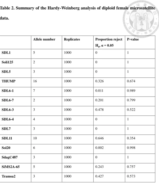
The microsatellite data from 244 females from 35 colonies were tested for violation of Hardy-Weinberg equilibrium (Table 1). I assessed significance using 1000 adjusted- bootstrap replicates. This analysis revealed that no linked locus rejected the null hypothesis. Control unlinked loci (Sol20, SdagC487, SiMS2A-65, and Tramsa2) did not deviate from Hardy-Weinberg equilibrium, as expected. The analysis data are in Table 2.
Although the focal loci did not reject the Hardy-Weinberg model, the result does not
exclude this SDL homologous region as the candidate. Analysis of only the female data for RIFA showed a similar result. The main evidence implicating the hypervariable region for RIFA is based on genotyping of diploid males, which was not possible for TFA. Given that there are probably many alleles at the sex locus in TFA, analysis of singlet microsatellite loci may not have enough power since some loci have only a few alleles.
3.1.3 The exact simulation p-value indicates that a sample size of 1.3 times the allele number is necessary to make the analysis significant.
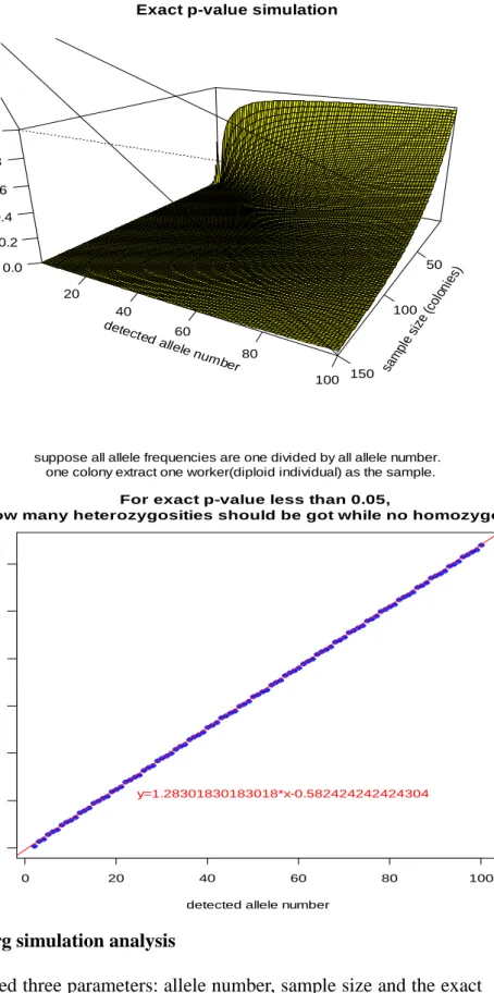
We next considered if the failure to reject Hardy-Weinberg equilibrium could have been due to the lack of statistical power. To test this possibility, I conducted a simulation with different allele numbers (1 to 100) and sample sizes (1 to 150) and then calculated the exact p-value (Fig. 2A). For this analysis, the exact p-value is the extreme probability that all extracted samples are heterozygous when in Hardy-Weinberg equilibrium. This simulation shows that the slope of detected allele number and the minimum needed sample size is about 1.3 if the type I error rate is fixed at 0.05 (Fig. 2B). I conclude that I would have enough power to find the candidate region if it is heterozygous in all samples and the sample size (colonies number) is about 1.3 times the actual allele number.
3.1.4 Analysis of heterozygosity of haplotype blocks potentially suggest that the region between THUMP to SDL6-4 as the candidate SDL locus.
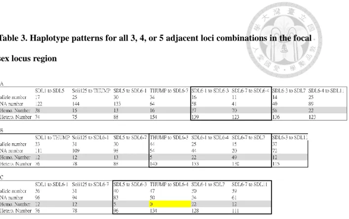
In the CSD mechanism, homozygosity at the region should never be observed in females. Building haplotype blocks may allow enumerating all the alleles. Therefore I built up haplotype blocks to do this. A haplotype is a group of genetic markers (SNP, microsatellite, etc), which is transmitted to the next generation together if there is no recombination. So it could be regarded as a genetic unit. Haplotype blocks consisting of 3, 4, or 5 neighboring microsatellite loci located near the SDL locus were examined in all
female data. Attempts at using >5 loci were unsuccessful because enough recombination occurred among individuals within colonies, thus precluding analysis. In this analysis only phased data was used and to reduce noise, the alleles (haplotypes) with missing data were excluded in the analysis despite reducing the sample size. The results (Table 3) show that only the region from THUMP to SDL6-4 was never homozygous. This never homozygous region only included 19 colonies and the random chance of obtaining no homozygotes for this haplotype was 0.119. This result only weakly suggests a candidate region.
3.2 Balancing selection is supported in the homologous seque nce in the hypervariable region.
3.2.1 The description of the hypervariable region and the nearby region and genes.
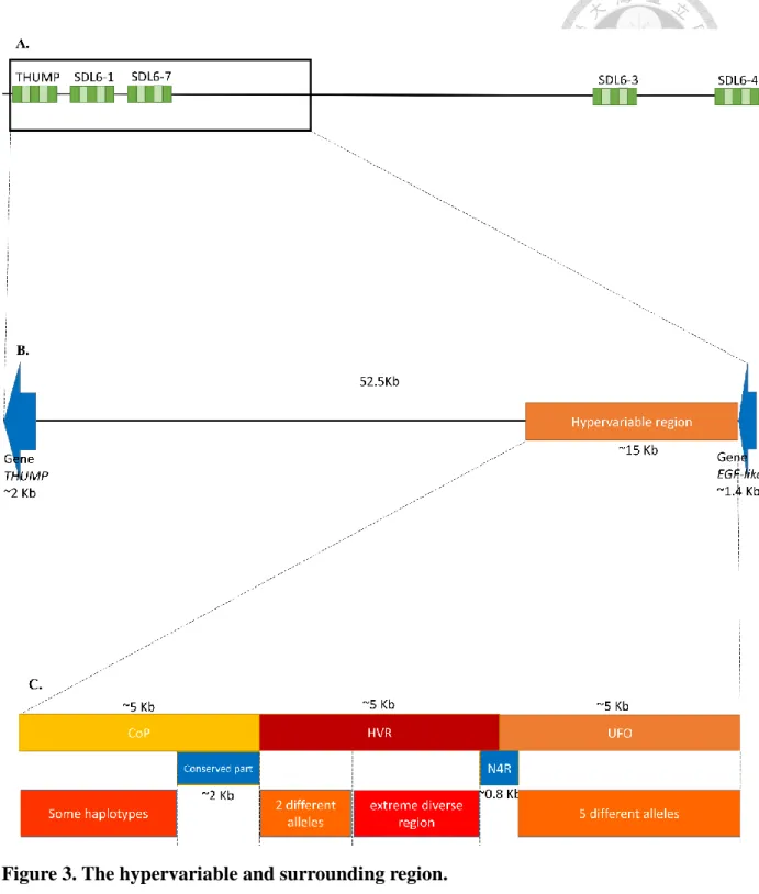
After aligning and comparing the sequences of TFA and RIFA together, the structure of this region which lacks homozygotes could be described (Fig. 3). The nucleotide diversity (π) and Tajima's D were also calculated (Table 4). Basically, like RIFA, the homologous hypervariable region (about 52.5 Kb) is between the same flanking genes THUMP (about 2 Kb) and EGF-like (about 1.5 Kb) and there are no other obvious genes in this range. In addition, based on two blocks of conserved sequences the hypervariable region was been divided into three sub-fragments: UFO, HVR and CoP. From the gene orientations, the first gene is EGF-like. This is a coding gene with epidermal growth factor-like domains. Then, next is one sub-fragment of the hypervariable region, UFO, which is about 5 Kb. There are several alleles here, each one being very different from the others. All sequences from TFA belong to the same allele family. A 0.8 Kb conserved non-coding region, N4R, follows. The next sub-fragment is HVR, including two parts.
The part closest to N4R is about 3 Kb, is an extremely diverse region, contains some large indels (INsertion/DELetion, more than 100 bp), and belongs to a few discrete clades spread among all samples. It is worth mentioning that one of the indels is shared by one RIFA sample and one TFA sample (Fig. 4). The other part is an about 2 Kb region and converges into 2 conserved alleles. Again, all TFA sequences are categorized into one of these two alleles. The sequences continuously converge into an about 2 Kb conserved region with relatively few SNPs and few indels. After this region is the CoP sub-fragment which has an about 3 Kb diverse region that is just less polymorphic than HVR. This is the region that is covered by allele sequence that the alignment software suggests (see method 3.1). The neighboring region is an about 37.5 Kb intervening region between the hypervariable region and the gene THUMP. These final two regions are relatively conserved and were not further investigated here.
3.2.2 Gene tree analyses support trans-species polymorphism (TSP) in the hypervariable region.
The homologous TFA hypervariable region sequence was compared to the RIFA sequence using blast. In the TFA draft genome, the blast results showed that HVR was similar to haplotype 3 of RIFA, but UFO and CoP which flank HVR was most similar to haplotype 1 of RIFA.
The phylogenetic tree could describe the relationship among the TFA and RIFA sequences and provide hints for exploring the sex locus under the CSD mechanism. If the hypervariable region is truly the only sex locus in TFA, then it should be under balancing selection. Strong balancing selection is often associated with TSP because old alleles were kept that can even exceed the species age. In contrast, if this region is unimportant (i.e., TFA evolved another locus for sex determination), most alleles in TFA should be lost by
drift or possible selective sweeps due to hitchhiking. In this case, TFA sequences should be an out-group to the RIFA alleles or derived from one of the RIFA alleles. Thus by examining phylogenetic trees of the candidate region, we can distinguish which hypothesis is more likely. The TSP phenomenon also could be caused by convergence, introgression and new speciation. Thus, in addition to the hypervariable region, I cloned 5 neutral sequences and compared them to exclude these three possibilities.
Thus far, 5 CoP sequences, 4 HVR sequence, 3 UFO sequences, 4 EGF-like sequences and 6 to 9 samples for each neutral sequence in TFA were cloned. Additionally, the existing TFA genome assembly sequence was added as another sequence set. These sequences were analyzed and phylogenic trees constructed for each phylogenic tree. In the phylogenic tree for EGF-like, there were 5 clades and 4 of 5 TFA sequences belonged to one of these. The other one looked different than others and was classified in another clade. There were 5 clades in the UFO tree and the distances between each other were relatively far. All TFA sequences obviously belonged to the same clade. The first part of HVR was most polymorphic and TFA sequences were spread among 3 clades in the tree.
The other part was separated into two clades and all TFA sequences were grouped into one of these. Although the CoP sequences also could be divided to two parts, the results were similar in that one of 6 TFA sequences was discrete from the others (Fig. 5C to Fig.
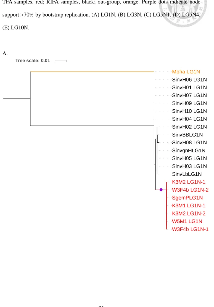
5H). In sum, the phylogenic trees of CoP, HVR and the gene EGF-like all exhibited the TSP phenomenon, even though an out-group was only available for EGF-like. This is consistent with our prediction. In contrast, all neutral sequences showed that the TFA sequences were in one cluster with no evidence for TSP (Fig. 6A to Fig. 6E). Together, these data indicate that in TFA, the hypervariable region shares some alleles with RIFA.
In contrast, the other regions cluster as a group from RIFA, even for a control region (LG3N) that was nearby, only <100 kb away.
In fact, part of intervening region (about 3.5 Kb with out-group sequence available) and the gene THUMP were analyzed with only one TFA sample, many RIFA samples and the out-group (Fig. 5A, 5B). The intervening region tree showed a similar result: the TFA sample is mixed within the RIFA clade despite only one sample, Although this cannot be considered as a solid evidence, this region is obviously different from the phylogenetic tree for the gene THUMP (which has with the same sample size) where the TFA sample is independent of the RIFA clade. This result indicates that the TSP phenomenon is in the hypervariable region and is attenuated to both sides, at least to the gene THUMP and the neutral region LG3N.
4. Discussion
In this study, I tested the homologous TFA SDL region by conducting Hardy- Weinberg tests, heterozygosity analysis, and examining the phylogenic trees of the target and neutral regions. Although my data are not definitive, the results from heterozygosity power analysis and phylogenic trees are consistent with the possibility that TFA also uses the homologous SDL locus for sex determination as RIFA does.
4.1 Structural similarity between TFA and RIFA at the SDL homology candidate region
I used 3 versions of the TFA genome sequence to assemble the SDL homology candidate region of TFA and found that it is similar to the structure of RIFA’s. All microsatellite loci and the genes in this region are in the same relative positions and direction. In the initial draft genome of TFA, the relative position of the hypervariable region could not be identified until the second version (PacBio version) was available.
This was because there were likely 3 different alleles at this locus preventing the software from assembling this region. This polymorphism phenomenon is consistent with the RIFA model.
The characteristics of each sub-region were also similar except the sub-fragment, UFO. In my TFA data, I only found one allele whereas many alleles were detected in RIFA. The lack of finding other alleles could be due to sampling bias, such as PCR bias.
For example, failed PCR and cloning would result in less sequenced alleles.
4.2 Information from single microsatellite markers are insufficient to confirm or refute the sex locus.
The Hardy-Weinberg test is a simple way to examine if the region is operating under the CSD mechanism because the expectation is that there should never be homozygous
females at the sex locus and reduced homozygosity at nearby linked loci. Analysis of the female data for each microsatellite locus revealed none with significant deviation from HW equilibrium. This result is not surprising because analysis of comparable female-only data from RIFA also showed a similar result. Thus, multilocus haplotype blocks were examined. I found that a haplotype block consisting of 5 microsatellites in the region from THUMP to SDL6-4 (which encompasses the hypervariable region in the SDL candidate region) was always heterozygous (p ≅ 0.12) using high quality, but low sample size data.
4.3 The highly diverse haplotypes at the SDL region in TFA.
If TFA uses a sl-CSD mechanism and the sex locus is orthologous to the SDL region in RIFA, then a prediction is that the SDL region in TFA would contain many haplotypes.
My results support this prediction. Based on microsatellite data of all samples, I found 115 all-loci haplotypes (with 10 homologous microsatellite makers) from 39 colonies.
Additionally, the observed haplotypes seem different in each colony. This indicates that the amount of shared haplotypes among colonies is very low despite most of the data coming from one population, Taichung Wuqi.
In RIFA, there are 10 sex alleles in Taiwan and each allele corresponds to 1 haplotype constructed from microsatellites in the SDL region. My results could imply that TFA has 47 sex alleles depends on the heterozygous power analysis (see table 3). Alternatively, new haplotypes may have been created by recombination since TFA’s arrival to Taiwan resulting in multiple haplotypes mapping to each sex allele. Recombinant haplotypes are more probable for TFA since they arrived more than 4 hundred years ago (Gotzek et al., 2015), compared to RIFA which arrived in Taiwan more recently (Ascunce et al., 2011).
Another possibility is that some microsatellites have mutated by expansion or contraction, and thus creating new haplotypes. Resolution of these possibilities will require cloning of
the locus and additional detailed sequence analysis of the region.
4.4 Balancing selection could be supported by the TSP phenomenon.
The sex locus should be under balancing selection which predicts that alleles could persist as trans-species polymorphisms (TSP). At the honeybee sex locus, TSP is also present in some related species (Cho et al., 2006). Cho et al showed that the type 2 csd alleles of A. mellifera are more similar to A. dorsata, suggesting balancing selection works at the honeybee sex determination locus. In addition, the major histocompatibility complex of vertebrates (Takahata and Nei, 1990) and the self-incompatibility locus of plants (Vekemans and Slatkin, 1994) also show the TSP phenomenon under balancing selection.
I tested whether the TFA alleles might exhibit TSP by sequencing three different sub- fragments of the hypervariable region, the gene EGF-like, and neutral regions LG1N, LG3N, LG5N1, LG5N4 and LG10N. Indeed, this analysis revealed that the alleles for hypervariable region and the gene EGF-like for TFA are dispersed in the phylogenetic tree with RIFA except the sub-fragment, UFO. Yet, the homologous sequence of the out- group could not be found, and consequently the trees of sub-fragments were unroot trees.
In contrast, none of the neutral regions exhibited the TSP phenomenon; all were clustered in one group which could be split from RIFA sequences.
Although consistent with balancing selection, TSP may also arise by recent speciation, introgression, and convergence. Recent speciation can be excluded because TFA is a basal lineage in the fire ants and split from the lineage leading to RIFA a long time ago (Gotzek et al., 2010; Pitts and McHugh Ross, 2005). Recent introgression is also unlikely because the two species are not known to hybridize where they overlap.
Convergence means the independent evolutional lineages have with similar features.
An argument against convergence is that evidence from another ant suggests that the sex locus may be ancient. In the ant V. emeryi, which uses 2 locus CSD, the location of one of the sex determination genes is close to the homologous hypervariable region and may suggest SDL is conserved from ancestral species. Thus, balancing selection is the most likely explanation.
The fact that V. emeryi uses 2-loci CSD raises an interesting possibility regarding sex determination evolution in ants. The second QTL locus maps to the homologous tra gene, which is homologous to the honeybee csd gene. One intriguing possibility is that fire ants in the native range actually use 2-locus sex determination, like V. emeryi, but because of the bottlenecks associated with fire ant invasions into the USA and subsequently elsewhere, there was loss of alleles at the tra locus. Consequently, the invasive range now only has single-locus CSD. This scenario, termed sex determination meltdown event, has been demonstrated for a parasitoid wasp, Cotesia rubecula (de Boer et al., 2012). If this is true, then the evolution of 2-locus sex determination followed by meltdown of one allele may suggest a mechanism of how CSD loci appear to "move"
during evolution.
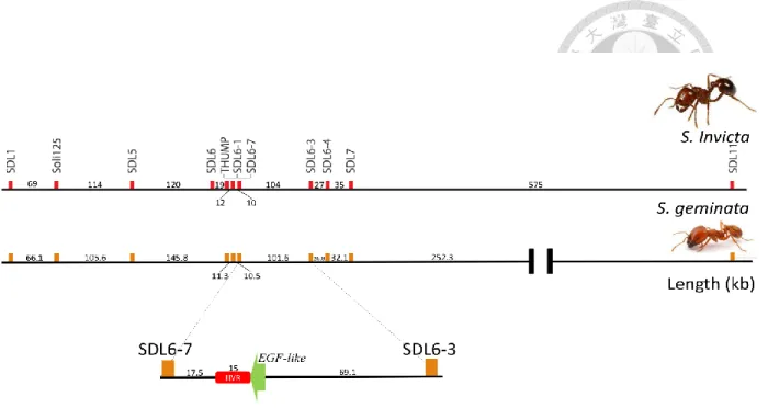
Figure 1. Comparison of the candidate sex locus within the SDL region of TFA and RIFA.
The TFA draft genome contains 3 overlapping fragments that align to the RIFA candidate sex locus. Using microsatellite loci which are linked to the RIFA SDL region as markers labels the homologous TFA SDL region. In addition to the hypervariable region (HVR) and the genes THUMP and EGF-like, the relative positions of all markers are similar between these two species. Only the SDL11 marker could not be confirmed because it is not assembled onto the same TFA contig as the other markers. Units are in kilobasepairs (kb).
A.
B.
Figure 2. Hardy-Weinberg simulation analysis
(A)The simulation examined three parameters: allele number, sample size and the exact p-value. (B) When the type I error is fixed at 0.05, the largest exact p-value is similar to a line described by Y = 1.28 * X - 0.58.
sample size (colonies) 50
100
150 detect
ed alle
le number 20
40
60
80
100 p-va
lue
0.0 0.2 0.4 0.6 0.8 1.0
Exact p-value simulation
suppose all allele frequencies are one divided by all allele number.
one colony extract one worker(diploid individual) as the sample.
0 20 40 60 80 100
020406080100120
For exact p-value less than 0.05,
how many heterozygosities should be got while no homozygosity
detected allele number
minimum needed sample size(colonies)
y=1.28301830183018*x-0.582424242424304
sample size (co lonies) 50
100
150 detect
ed allele num ber 20
40
60
80
100
p-value
0.0 0.2 0.4 0.6 0.8 1.0
Exact p-value simulation
suppose all allele frequencies are one divided by all allele number.
one colony extract one worker(diploid individual) as the sample.
0 20 40 60 80 100
020406080100120
For exact p-value less than 0.05,
how many heterozygosities should be got while no homozygosity
detected allele number
minimum needed sample size(colonies)
y=1.28301830183018*x-0.582424242424304
Figure 3. The hypervariable and surrounding region.
(A) Schematic of genomic region where all TFA females are never homozygous. This region encompasses 5 microsatellite markers, THUMP, SDL6-1, SDL6-7, SDL6-3 and SDL6-4. (B) Zoom of the region between the two genes, THUMP and EGF-like. (C) Detailed view of the region including CoP, HVR and UFO. Red, orange, and yellow are a rough indication of the diversity within each sub-region.
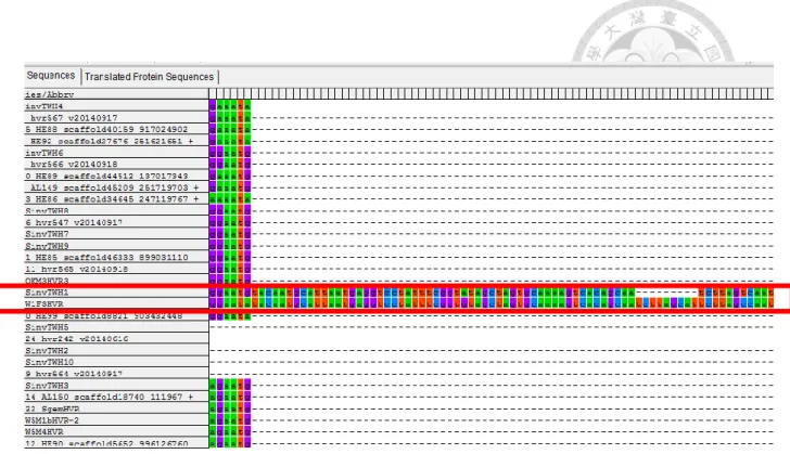
Figure 4. The shared “insertion” between TFA and RIFA.
A shared “insertion” between a TFA (W1F3HVR ) and a RIFA (SinvTWH1) sample (red box). No other samples share this insertion. The length of this insertion is 167 bp.
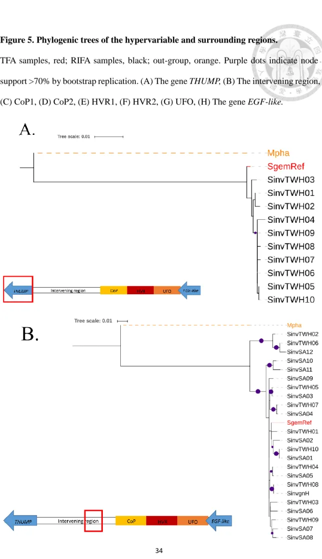
Figure 5. Phylogenic trees of the hypervariable and surrounding regions.
TFA samples, red; RIFA samples, black; out-group, orange. Purple dots indicate node support >70% by bootstrap replication. (A) The gene THUMP, (B) The intervening region, (C) CoP1, (D) CoP2, (E) HVR1, (F) HVR2, (G) UFO, (H) The gene EGF-like.