An Energy-Conserved On-Demand Data Broadcasting System
Jiun-Long Huang
Department of Electrical Engineering National Taiwan University
Taipei, Taiwan, ROC
E-mail:[email protected]
Wen-Chih Peng
Dept. of Computer Sci. and Info. Eng.
National Chiao-Tung University Hsinchu, Taiwan, ROC E-mail:[email protected]
ABSTRACT
We propose in this paper an energy-conserved on-demand data broadcasting system by employing the data indexing technique. We also propose algorithm AIDOA to adjust the degree of buckets according to system workload. Ex- perimental results show that algorithm AIDOA is able to greatly reduce power consumption at the cost of slight in- crement in average access time and adjust the index and data organization dynamically to adapt to change of system workload.
Categories and Subject Descriptors
H.2.4 [Database Management]: Systems
General Terms
Algorithms, performance
Keywords
Data indexing, on-demand data broadcasting, energy con- servation, mobile information system
1. INTRODUCTION
As shown in [5][6], only a modest improvement (about 20% ∼ 30%) in battery lifetime is expected in the next few years.
Hence, energy conservation is raised as a key factor of the design of mobile devices. Most devices can operate in two modes: active mode and doze mode. Many studies show that the power consumed in active state is much higher than that consumed in doze mode. As a consequence, the mobile devices should stay in doze mode as long as possible to re- duce power consumption.
To evaluate the effect of data indexing algorithms on energy conservation, tuning time, which is defined as the time that a mobile device operates in active mode in order to retrieve
MDM 2005 05 Ayia Napa Cyprus c
°2005 ACM 1-59593-041-8/05/05....$5.00
Permission to make digital or hard copies of all or part of this work for personal or classroom use is granted without fee provided that copies are not made or distributed for profit or commercial advantage and that copies bear this notice and the full citation on the first page. To copy otherwise, to republish, to post on servers or to redistribute to lists, requires prior specific permission and/or a fee.
Ii(1) Ii(2) Ii(d) Di(1) Di(2) Di(d)
ISi DSi
Bucketi
Figure 1: Index structure
a data item, is introduced in [3]. Since employing data in- dexing will unavoidably introduce some overhead in access time1, the data indexing algorithms should reduce tuning time as much as possible at the cost of producing an accept- able increment in access time. Fortunately, since the size of an index item is usually much smaller than that of a data item, such increment is usually small.
The authors in [4] proposed an indexing approach for on- demand data broadcast systems. As shown in Figure 1, the proposed broadcast program is made up of a series of buckets and each bucket consists of one index segment and one data segment. The number of data items in a bucket is called the degree of the bucket. A data segment contains a series of data items, and an index segment consists of the index items of the data items in the corresponding data segment.
The information in an index item, say Ii(1), consists of the identifier of the corresponding data item Di(1), the data size of Di(1) and the time that Di(1) in bucket i will be broadcast on the broadcast channel. In addition, by the information in the current index segment, a mobile device is able to determine the broadcast time of the index segment of the next bucket.
Although it shows in [4] that inserting index items into the broadcast program is able to significantly reduce the average tuning time at the cost of slight increment in average access time, however, the proposed data indexing method proposed in [4] has the following drawbacks:
• Does not consider power consumption of turning on and turning off the WNIs.
• Does not adapt to change of system workload
1Average access time is defined as the average time elapsed from the moment a client issues a query to the point the desired data item is read.
Fetcher
Cache
Scheduler Request Queue Ready Queue
Current Broadcast Bucket Internet
Server Server
Program Generator
Data Requests Index and
Data Items
Broadcast Channel Request Channel
Pending List
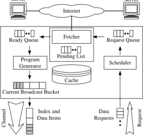
Figure 2: System architecture
In view of this, we propose in this paper an energy-conserved on-demand data broadcasting system by employing the data indexing technique. Different from the prior work on data indexing on on-demand data broadcasting, power consump- tion of turning on and turning off the WNIs is considered.
We first analyze the access time and tuning time of data re- quests and propose algorithm AIDOA to adjust the degree of buckets according to system workload. In essence, algo- rithm AIDOA consists of two phases, statistics collection phase and adjustment phase, and switches back and forth between these two phases. The system collects some statistic information of all served data requests in statistics collection phase, and the information is used to adjust the degree of buckets in adjustment phase according to the derived ana- lytical results. Several experiments are then conducted to evaluate the performance of algorithm AIDOA. Experimen- tal results show that due to the dynamic adjustment on degree, scheme using algorithm AIDOA outperforms other schemes with static degree in most cases and is able to adapt to change of system workload.
The rest of this paper is organized as follows. Section 2 describes the power consumption model and client access protocol adopted in this paper. Based on the analytical model, we propose algorithm AIDOA in Section 3. Several experimental results are shown in Section 4 to evaluate the performance of algorithm AIDOA. Finally, Section 5 con- cludes this paper.
2. PRELIMINARIES
2.1 Power Consumption Model
Denote the time for a mobile device to switch the WNI from active mode to doze mode as TOnand the time to switch the WNI from doze mode to active mode as TOf f. To evaluate the power consumption of turning on and turning off the WNIs, we assume that the power consumption of a mobile device spending in time interval TOn(respectively, TOf f) is equal to that of a mobile device staying in active mode for time α1× TOn(respectively, time α2× TOf f). Similar to [8], the values of α1 and α2 can be obtained by profiling.
ISi DSi ISi+1 DSi+2 ISj DSj
tStart tEnd
Probe Bucket Search Bucket Retrieval Bucket
Figure 3: Categories of buckets
Denote the traditional (i.e., without considering the turning- on and turning-off time of WNIs) average tuning time of a data request as TT uning. For a data request, we also let TOn
and TOf f be the average times for a mobile device spending in turning on and turning off the WNI. Hence, to evaluate the overall power consumption, we define the effective tun- ing time of a data request as TT uningEf f. = TT uning+ n1× α1× TOn+ n2× α2× TOf f, where n1 and n2 are the numbers of times of turning on and turning off the WNI, respectively, and TT uningis the traditional tuning time. To ease the pre- sentation, we use the term tuning time to represent effective tuning time, and assumes α1 = α2 = 1 in the rest of this paper.
2.2 Client Access Protocol
After submitting a data request, a mobile client will behave according to the employed client access protocol to retrieve the desired data item. In this paper, we adopt the client access protocol described in [7], and the protocol consists of the following phases.
• Initial probe phase: After submitting a data request, the mobile device tunes to the broadcast channel and listens on the broadcast channel to wait for the ap- pearance of an index segment.
• Index search phase: The mobile device enters index search phase after receiving an index segment. In in- dex search phase, the mobile device determines whether the desired data item will be broadcast in the cor- responding data segment. If not, the mobile device will switch to doze mode and then switch back to ac- tive mode when the next index segment is broadcast.
Otherwise, the mobile device will enter data retrieval phase.
• Data retrieval phase:
If the desired data item will be broadcast in the current data segment, the mobile device will calculate the time that the desired data item will be broadcast from the current index segment and switch to doze mode. Then, when the desired data item is broadcast, the mobile device will switch back to active mode to retrieve the desired data item.
Consider the example shown in Figure 3 that a mobile device submits a data request. tStart is the time that the mobile device starts to listen on the broadcast channel after submit- ting the data request, and tEndis the time that the mobile device receives the desired data item. From the perspective of the mobile device, the buckets within the time interval from tStart to tEnd can be divided into the following three categories according to the above three phases:
• Probe bucket: The bucket which tStartlies on is called the probe bucket. In Figure 3, Bucket(i) is the probe bucket. There is exactly one probe bucket for a data request.
• Search bucket: The bucket whose index segment is retrieved by the mobile device and whose data seg- ment is skipped by the mobile device is call the search bucket. In Figure 3, Bucket(i + 1), Bucket(i + 2),
· · · , Bucket(j − 1) are all search buckets. For a data request, there may be zero, one or multiple search bucket(s).
• Retrieval bucket: The bucket which tEnd lies on is called the probe bucket. That is, retrieval bucket is the bucket where the mobile device retrieves the de- sired data item. In Figure 3, Bucket(j) is the retrieval bucket. For a data request, there is exactly one probe bucket. In addition, the probe bucket and the retrieval bucket of a data request may be the same or different.
3. AIDOA: ADAPTIVE INDEX AND DATA ORGANIZING ALGORITHM
We propose in this section algorithm AIDOA (standing for Adaptive Index and Data Organizing Algorithm) to adjust the degree of buckets according to the system workload. Ba- sically, algorithm AIDOA consists of two phases: statistics collection phase and degree adjustment phase, and switches between statistics collection phase and degree adjustment phase periodically. In statistics collection phase, the system will keep track of information of all data requests and the recorded information will be used to guide the adaptation procedure in the successive execution of adjustment phase.
3.1 Types of Data Requests
To facilitate the design of algorithm AIDOA in the following subsections, a data request is categorized by (1) the relation- ship between its probe bucket and its retrieval bucket and (2) the relationship between its tStartand its tEnd. Accord- ing to the relationship of the probe and the retrieval buckets, a data request can categorized in to the following two types.
Type I: The probe and the retrieval buckets are the same.
Type II: The probe and the retrieval buckets are the different.
Now, consider the relationship of tStart and tEnd of a data request. According to the employed client access protocol, in a Type I data request, tStartmust be located in the index segment. Otherwise, tStartand tEndwill not be in the same bucket, and such result conflicts with the definition of Type I. On the other hand, a Type II data request can be further divided into the following two subtypes according to the location of tStart.
Type II.I: tStart is in the index segment.
Type II.II: tStart is in the data segment.
3.2 Statistics Collection Phase
In each execution of statistics collection phase, the system will collect statistic information of all data requests which
have been served in the current execution of statistics col- lection phase. A data request is served when the desired data item has been broadcasted.
Two data structures, StatIand StatII, are defined to stored the collected information of data requests belonging to Type I, Type II (including Type II.I and Type II.II), respectively.
The details of StatI and StatII are as follows.
Details of StatI
• ReqNo: The number of Type I data requests served in the current statistics collection phase
• AggAT: Aggregated Access Time of all Type I data re- quests served in the current statistics collection phase
• AggTT: Aggregated Tuning Time of all Type I data re- quests served in the current statistics collection phase Details of StatII
• ReqNo: The number of Type I data requests served in the current statistics collection phase
• AggATP/AggTTP: Aggregated Access/Tuning Time of Probe buckets of all Type II data requests served in the current statistics collection phase
• AggATS/AggTTS: Aggregated Access/Tuning Time of Search buckets of all Type II data requests served in the current statistics collection phase
• AggATR/AggTTR: Aggregated Access/Tuning Time of Retrieval buckets of all Type II data requests served in the current statistics collection phase
Each field, except ReqN o of StatIand StatII, has an aver- age version by replacing prefix Agg to Avg. For example, the field AvgAT of StatI indicates the average access time of all Type I data requests served in the current statistics collection phase. We also define the structure Request to indicate multiple data requests which are merged together.
Elements in the request queue, pending list and the ready queue are all instance of structure Request. An instance of structure Request is said in the system when it is in the request queue, pending list or the ready queue. The details of structure Request are as follows.
Details of structure Request
• ReqNo: The number of data requests which are merged together and are represented by the Request structure.
• AvgTIS : Average Time In Search buckets of the data requests that the Request structure represents.
After receiving a data request, the system first determines the type of this data request. If the data request is belonging to Type I, the system calculates the contributions of the data request on the aggregated average and tuning time and updates StatI accordingly. Since being able to be served by the current bucket, a Type I data request will neither be merged into a structure Request nor be inserted into the request and ready queues and pending list.
On the other hand, when the data request is belonging to Type II, the system first checks whether it can be merged into an instance of structure Request in the system. If yes,
the system updates the fields (i.e., ReqN o and AvgT IS) of the instance of structure Request accordingly. Otherwise, the system creates a new instance of structure Request and inserts the instance into the request queue. Finally, the system calculates the contribution on aggregated access time and tuning time of the probe bucket of the data request, and updates StatII accordingly.
While an instance of Request, say r, is retrieved from the ready queue, the system first calculates the average number of search buckets that each data request represented by r has by
AvgSBN o ← Bucket(j).start − r.AT IS d × (SD+ SI) .
Then the system calculates the time that the desired data item of r can be retrieved (i.e., tEnd). Finally, with tEnd, the system calculates the aggregate contributions of the probe buckets of all data requests represented by r on the aggre- gated access time and tuning time, and updates StatII.AggAT R and StatII.AggT T R accordingly.
3.3 Degree Adjustment Phase
In each execution of degree adjustment phase, the system will adjust the degree (i.e., the value of d) of buckets accord- ing to the statistic information collected in the precedent execution of statistics collection phase. Let TAccess(d) and TT uning(d) be the average access time and average tuning time, respectively, when the degree of the broadcast pro- grams is d. For each field, the value of the average ver- sion is equal to the value of the aggregate version divided by the number of data requests. For example, the value of StatI.AvgT T is equal to StatStatI.AggT T
I.ReqN o. Then, we have TAccess(d)
= WI× (StatI.AvgAT ) + WII×
(StatII.AvgAT P + StatII.AvgAT S + StatII.AvgAT R), and
TT uning(d)
= WI× (StatI.AvgT T ) + WII×
(StatII.AvgT T P + StatII.AvgT T S + StatII.AvgT T R), where WI and WII are the weights of Type I and Type II data requests, respectively. The values of WI and WII are defined as the ratios of the numbers of Type I and Type II data requests and are equal to Stat StatI.ReqN o
I.ReqN o+StatII.ReqN oand
StatII.ReqN o
StatI.ReqN o+StatII.ReqN o, respectively. In addition, TOverAll(d) is adopted as the metric of the system performance when the degree of the broadcast programs is d, and is defined as
TOverAll(d) = β × TAccess(d) + (1 − β) × TT uning(d), where β is the weight of TAccess(d). The objective of de- gree adjustment phase is to determine the value of d to minimize TOverAll(d1). However, since globally minimizing TOverAll(d) is difficult, algorithm AIDOA is designed to find the new value of d, say d1, where TOverAll(d1) is local min- imum where TOverAll(d1) is smaller than TOverAll(d1+ 1) and TOverAll(d1− 1). Since the exact values of TAccess(d1) and TT uning(d1) where d16= d cannot be obtained from the statistic information, we adopt the following approximation method to estimate TAccess(d1) and TT uning(d1).
Let StatdI1 and StatdII1 be the approximations of the values of structure StatI and StatIIwhen the degree of buckets is d1. Then, we have the following lemmas:
Lemma 1 StatdI1.AvgAT and StatdI1.AvgT T can be ap- proximated by
StatdI1.AvgAT = StatI.AvgAT + (d1− d) ×SI
B, and
StatdI1.AvgT T = StatI.AvgT T, respectively.
Lemma 2 StatdII1.AvgAT P and StatdII1.AvgT T P can be ap- proximated by
Statd1II.AvgAT P
= SI
SI+ SD
× Statd1II.I.AvgAT P + SD
SI+ SD
× Statd1II.II.AvgAT P,
and
Statd1II.AvgT T P
= SI
SI+ SD
× Statd1II.I.AvgT T P + SD
SI+ SD
× Statd1II.II.AvgT T P,
respectively, where
StatdII.I1 .AvgAT P = StatII.AvgAT P +(d1−d)×
µSI
B +SD
B
¶ ,
StatdII.I1 .AvgT T P = StatII.AvgT T P + (d1− d) ×SI
B, StatdII.II1 .AvgAT P = StatII.AvgAT P + (d1− d) ×SD
B and
StatdII.II1 .AvgT T P = StatII.AvgT T P + (d1− d) ×SD
B .
As mentioned in Lemma 2, setting the degree of buckets will increase the numbers of index and data items in each probe bucket of Type II data requests by d1− d. Suppose that these extra index and data items are from the search buckets. Then, we have
Lemma 3 StatdII1.AvgAT S and StatdII1.AvgT T S can be ap- proximated as
StatdII1.AvgAT S = AvgSBN o1× d1×(SI+ SD)
B ,
and
StatdII1.AvgT T S = AvgSBN o1× µ
d1×SI
B + TOf f+ TOn
¶ , where
AvgSBN o1 = StatII.AvgAT S × B
d1× (SI+ SD) −d1− d d1
, respectively.
Lemma 4 StatdII1.AvgAT R and StatdII1.AvgT T R can be ap- proximated as
StatdII1.AvgAT R = StatII.AvgAT R + (d1− d) ×SI
B, and
StatdII1.AvgT T R = StatdII1.AvgT T R, respectively.
0 0.5 1 1.5 2 2.5 3
5 10 20 30 40 50 60
Turning-on and Turning-off Time (ms)
Average Access Time (sec)
Static-2 Static-8 AIDOA
(a) Average Access Time
0 0.2 0.4 0.6 0.8 1 1.2 1.4
5 10 20 30 40 50 60
Turning-on and Turning-off Time (ms)
Average Tuning Time (sec)
Static-2 Static-8 AIDOA
(b) Average Tuning Time Figure 4: The effect of turning-on and turning-off time
We then devise procedure DegreeAdjustment to find the value of d1 where TOverAll(d1) is local minimum. In pro- cedure DegreeAdjustment, the system first checks whether increasing or decreasing the value of degree will reduce the value of TOverAll(d1). After that, the system repeatedly in- creases or decreases the value of degree by one until TOverAll(d1) is local minimum. Finally, the system sets the value of de- gree to the return valued of procedure DegreeAdjustment.
4. PERFORMANCE EVALUATION 4.1 Simulation Model
In order to evaluate the performance of the proposed degree adjustment method in algorithm AIDOA, the algorithm pro- posed in [4] (referred to as algorithm Static) is modified to integrated into the proposed system. Hence, the difference between algorithm AIDOA and algorithm Static is on the ability of adjusting the degree of buckets. Based on algo- rithm Static, we devise two schemes, Static-2 and Static-8 which set the degree of buckets to two and 8, respectively, and the values of degree of buckets are fixed throughout the simulation. In addition, scheme AIDOA employs algorithm AIDOA and initializes the degree of buckets to two. Hence, scheme AIDOA will dynamically adjust the degree of buck- ets according to system workload. Note that all these three schemes employ server cache and asynchronous I/O to elimi- nate performance degradation caused by the data item fetch time.
4.2 Effect of Turning-on and Turning-off Time of WNIs
The effect of turning-on and turning-off time of WNIs is measured in this subsection and the experimental results are given in Figure 4. In this experiment, we assume that TOn= TOf f and set the value of TOnand TOf f from 5ms to 60ms. As shown in Figure 4a, the values of TOn and TOf f
do not affect average access time in scheme Static-2 and scheme Static-8. It is because that in these two schemes, degrees of broadcast buckets are static, and the values of TOnand TOf f do not affect the organizations of broadcast programs. On the other hand, although scheme AIDOA is able to dynamically adjust the degree of buckets, the in- fluence of TOnand TOf f on average access time of scheme AIODA is small since the size of index items is much smaller than that of data items.
Consider average tuning time of these schemes shown in Figure 4b. Since the benefit of increasing the value of de- gree is in proportion to the values of TOnand TOf f, scheme
Static-2 performs well when TOn and TOf f are small. On the contrary, scheme Static-8 outperforms scheme Static-2 in the case with large TOnand TOf f. Although producing more power consumption in the probe bucket than scheme Static-2 does, scheme Static-8 is still able to reduce over- all power consumption since being able to greatly reduce the power consumption on turning-on and turning-off the WNIs by reducing the average number of search buckets.
On the other hand, with dynamic adjustment in the degree, scheme AIDOA is able to determine a suitable value of de- gree for current system workload, and hence outperforms scheme Static-2 and scheme Static-8 in most cases.
5. CONCLUSION
In this paper, we analyzed the access time and tuning time of data requests and proposed algorithm AIDOA to adjust the degree of buckets according to system workload. To fa- cilitate scheme AIDOA, we also devised an approximation method to estimate the effect of increasing and decreasing the values of degree. Experimental results showed that algo- rithm AIDOA is able to greatly reduce power consumption at the cost of slight increment in average access time and dy- namically adjust the index and data organization to adapt to change of system workload.
6. REFERENCES
[1] M. Agrawal, A. Manjhi, N. Bansal, and S. Seshan.
Improving Web Performance in Broadcast-Unicast Networks. In Proceedings of the IEEE INFOCOM Conference, March-April 2003.
[2] D. Aksoy and M. J. Franklin. Scheduling for Large-Scale On-Demand Data Broadcasting. In Proceedings of IEEE INFOCOM Conference, pages 651–659, March 1998.
[3] T. Imielinski, S. Viswanathan, and B. R. Badrinath.
Data on Air: Organization and Access. IEEE Transactions on Knowledge and Data Engineering, 9(9):353–372, June 1997.
[4] S. Lee, D. P. Carney, and S. Zdonik. Index Hint for On-demand Broadcasting. In Proceedings of the 19th IEEE International Conference on Data Engineering, March 2003.
[5] E. Shih, P. Bahl, and M. J. Sinclair. Wake on Wireless:
An Event Driven Energy Saving Strategy for Bettery Operated Devices. In Proceedings of the 8th
ACM/IEEE International Conference on Mobile Computing and Networking, September 2002.
[6] M. A. Viredaz, L. S. Brakmo, and W. R. Hamburgen.
Energy Management on Handheld Devices. ACM Queue, 1(7):44–52, October 2003.
[7] J. Xu, W.-C. Lee, and X. Tang. Exponential Index: A Parameterized Distributed Indexing Scheme for Data on Air. In Proceedings of the 2nd ACM/USENIX International Conference on Mobile Systems, June 2004.
[8] H. Zhu and G. Cao. A Power-Aware and QoS-Aware Service Model on Wireless Networks. In Proceedings of IEEE INFOCOM Conference, March 2004.