Design and Analysis of the Floating Kuroshio Turbine Blades

(1)

Design and Analysis of the Floating Kuroshio Turbine Blades

Fang-Ling Chiu^#1, Sin-An Lai^#2, Chi-Fang Lee^*3, Yu-An Tzeng^#4, Ching-Yeh Hsin^#5

# Dept. of Systems Engineering and Naval Architecture, National Taiwan Ocean University, 2, Pei-Ning Rd., Keelung, Taiwan 20224

1b233380@hotmail.com

2sinanlai.sal@gmail.com

4yuann.tzeng@gmail.com

5cy_hsin@hotmail.com

* CR Classification Society, 8th Fl., No.103, Sec. 3, Nanking E. Rd., Taipei, Taiwan 10491

3chifang@crclass.org

Abstract— The most common devices used for extracting the ocean current energy are the current turbines. Most people use the wind turbine blade design methods for the horizontal axis current turbine design; however, the current turbines operate in the water, and their physical behaviours are more like marine propellers. In this paper, two turbine blade design procedures are adopted. The first design procedure is similar to the propeller designs, and the second design procedure is to use Genetic Algorithm and boundary element method (BEM) to find a geometry which can provide the maximum torque. After completing the designs, hydrodynamic performances of the marine current turbine are then computed and analysed by the potential flow BEM and the viscous flow RANS method. The computational results show the geometries designed by the presented procedures can not only satisfy the hydrodynamic design goal, but also predict the delivered power very close to the experimental data. After the blade performance meets the design target, the performances of designed 20kw floating type Kuroshio turbine including the floating body at different operation conditions are demonstrated in the paper. Also, the structural strength of the turbine blade is computed by FEM, and the results are evaluated to see if the design complies the rule requirements.

Keywords—Kuroshio, current turbine blade design, boundary element method, RANS, FEM

I. INTRODUCTION

With the international highly attention to all kinds of energy issues, Taiwan is bound to examine the state of energy problem in the country. Since Taiwan currently does not have exploitation of non-renewable energy sources, it must rely on foreign imports and lack of the ability to supply energy on its own. In this situation, the application of renewable energy is another solution to the energy problem. There are many types of renewable energy, such as solar power and wind power that have been used successfully. However, from the point of view of the country's use of electricity, ocean current power generated from ocean energy is not affected by seasonal and weather factors. It can provide stable energy, and it is a very good choice as a base-load energy resource. The Kuroshio that flows through the outer seas of Taiwan is the ocean current that begins from Philippines and crosses through Taiwan and flows along Japan in the northeast direction. Two most

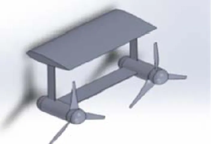
common devices used for extracting the ocean current energy are the horizontal axis current turbine and the vertical axis current turbine, and the power generation system presented in this paper is a floating Kuroshio turbine (FKT, as shown in Fig. 1) which is a horizontal axis current turbine developed using the Kuroshio Current as its energy source.

Fig. 1 The computer depiction of the 20kw Floating Kuroshio Turbine.

In this paper, the design procedure and performance analysis of the FKT are presented. First of all, the design target of this generator must be established. The generator designed in this paper is based on two horizontal shaft generators and must reach 20kW of power generation. In other words, a single-sided turbine must achieve a design target of at least 10 kW. Most people use the wind turbine blade design methods for the horizontal axis current turbine design;

however, the current turbines operate in the water, and their physical behaviours are more like marine propellers. In this paper, two turbine blade design procedures are adopted. The first design procedure is similar to the propeller designs, and lifting line method [1-2], lifting surface design method [3], and boundary element method [4] are used. The second design procedure is to use Genetic Algorithm and boundary element method (BEM) [5] to find a geometry which can provide the

(2)

maximum torque, and also used to design chord-length distribution. After completing the blade geometry designs, both the BEM and the viscous flow RANS method [6] are applied to the analysis of performances of current turbines to confirm the designs. The performances were calculated based on a 1/5 scale of 20kW demonstration unit; however, the experimental unit was tested with a 1/25 scale at NTU (National Taiwan University) towing tank. In this paper, we also present the comparison between computational results and experimental data, and the comparison shows that the geometries designed by the presented procedures can not only satisfy the hydrodynamic design goal, but also predict the delivered power very close to the experimental data

After confirming that the blade performance meets the design target, we further investigate FKT more comprehensively. It is no longer only to discuss the performance of the turbine blades only, but the effects on the turbine performance after adding the floating body. Also the overall FKT performances were simulated under different conditions during operations, such as breakdown of one side turbine. After completing the blade hydrodynamic analysis, a series of structural strength verifications are performed by finite element method (FEM) to check whether the design meets regulatory requirements after adding the safety factor.

II. HYDRODYNAMIC DESIGNS AND VALIDATIONS

Before presenting the design procedure, we first introduce several important coefficients related to the turbine performance. These coefficients are the tip speed ratio (TSR), thrust coefficient (CT ), torque coefficient (CQ) and power coefficient (CPW). They are defined as follows.

2

2 3

2 C 1 2

1 1

2 2

x T

W

Q PW Q

F TSR nR

V AV

P

C Q C TSR C

AV R AV

π

ρ

ρ ρ

∞ ∞

= =

= = = ×

(1)

The presented FKT design is completed via two major design processes. Since the ocean current turbine operates in water, its physical characteristics are more similar to those of marine propellers. Therefore, the design of FKT is first carried out by a process similar to the propeller design. The lifting line method and Lagrange multiplier method is first used to obtain optimum circulation distribution, and then lifting surface theory help us to get blade geometry, namely, the pitch and camber distribution. The second step is based on the genetic algorithm method. The goal of this procedure for the FKT is to achieve the maximum CQ (maximum torque and power). A procedure that is conceived and developed by the genetic algorithm method to adjust the pitch and camber distributions to reach our goal. The optimization of geometry parameters in the genetic algorithm computation process is performed by the boundary element method (BEM) because its efficient computational time. The potential flow BEM used here is a

self-developed, perturbation potential based boundary element method, and a wake alignment numerical scheme is established for the current turbine. Table 1 shows the FKT geometry parameters. Detail design procedure was presented in the last AWTEC conference [7].

TABLE 1

THE GEOMETRIC PARAMETERS OF THE 20KWFKT Foil Geometry NACCA66/ a=0.8 meanline

Diameter(m) 5

Rotational speed(rps) 0.5

Inflow velocity(m/s) 1.5

Fig. 2 Blade geometry of the 2-blade design along with and the results of RANS and BEM analysis.

(3)

Fig. 5 Computational results of the analysis of the three different blade numbers, and the position marked by the black line is the design point.

After the blade geometry was designed, we also designed different numbers of blades and hydrodynamic performances are also computed and analysed by BEM and RANS method for 2, 3, and 4 blades respectively. The RANS computations are carried out by the commercial CFD software STAR- CCM+. Fig. 2 shows blade geometry of the 2-blade design along with and the results of RANS and BEM analysis. Fig. 3 and Fig. 4 show those of 3-blade and 4-blade. Fig. 5 compares the results of the analysis of the three different blade numbers, and the position marked by the black line is the design point.

It can be seen that 3-blade is the best at the design point and is also the most stable one.

TABLE2

THE FORCE,TORQUE AND POWER COEFFICIENT OF THE DESIGNED 20KW FLOATING TYPE CURRENT TURBINE.

CT C_Q C_PW

BEM 0.70740 0.07905 0.41390

RANS 0.75950 0.08501 0.44510

F x Q P W

BEM 15594.74 4356.67 13686.73

RANS 16743.29 4685.14 14718.44

A. Computational Results of Single Turbine

After the final design of the blade was completed, the performance was computed with a 1/5 scale 20kW demonstration unit (as shown in Fig. 1). The diameter of blade is 5m, the rotation speed is 0.5rps, and the inflow is set as 1.5m/s, and number of the blades is 3 (Table 1). The performance is calculated by potential flow BEM and viscous flow RANS method, and the results are shown in Table 2.

From Table 2, one can see that either the BEM method or the RANS method, the output powers show that this design meets the design target of 10 kW for each turbine.

Fig. 1 The FKT is belong to the design of contra-rotation propeller.

TABLE3

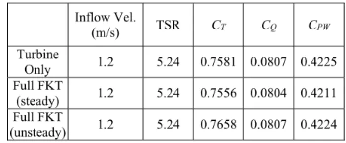
THE FORCE,TORQUE AND POWER COEFFICIENT OF THE FKT.

Inflow Vel.

(m/s) TSR CT CQ CPW

Turbine

Only 1.2 5.24 0.7581 0.0807 0.4225 Full FKT

(steady) 1.2 5.24 0.7556 0.0804 0.4211 Full FKT

(unsteady) 1.2 5.24 0.7658 0.0807 0.4224

B. Overall FKT Performance Analysis

The objects discussed in the previous sections are the design and performance of FKT blade geometry. In this section, the overall performance of the FKT is discussed.

Because the FKT is composed of a floating body and two turbines, and the rotational direction of each turbine is opposite to each other (shown in Fig.6). In order to understand the overall FKT unit performance, we have computed forces of FKT at a slower inflow speed, 1.2m/s, under the following conditions:

 Single turbine,

 With the floating body, and using steady RANS

 With the floating body, and using unsteady RANS (URANS). The mean values are taken for the comparison.

The reason to use both RANS and URANS for computations is to double check our computational results. The computed performances on each turbine is shown in Table 3, and it is obvious that whether there is a floating body or not, the differences are not large. We then investigate the influence of the floating body. Fig. 7 shows the flow field at different locations upstream of turbine blades with and without a floating body, and the distances upstream are 0.3m, 0.2m, and 0.1m respectively. From Fig. 7, one can see that the flow field at 0.3m upstream is obviously affected by the floating body;

however, the influence of floating body gradually decreased.

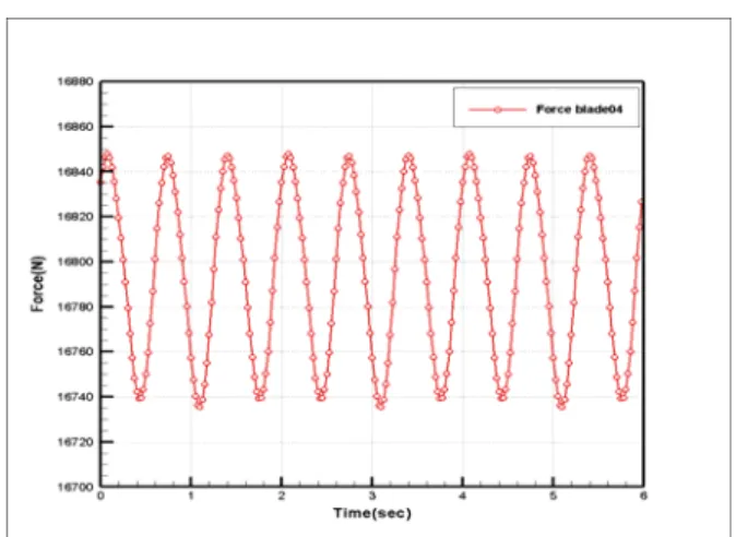
The flow field 0.1m upstream shows the floating body has almost no effect. We then look into the forces on each blade as it rotates (Fig. 8), and the force variations on each blade is

(4)

obviously affected by the floating body and the struts. The magnitude of force variation on each blade is about 2%. Fig. 9 then shows the total force on one turbine, which is the sum of forces on three blades as they rotate, and the force fluctuation is only 0.6%. Therefore, we can confirm again that the influence of the floating body is not significant on both forces and flow field.

Without a floating body With a floating body

0.3m upstream 0.3m upstream

Fig. 7 The flow field at different locations upstream of turbine blades with and without a floating body

Fig.8 Forces on each blade as it rotates, and the force variations on each blade is obviously affected by the floating body and the struts.

Fig.9 The total force on one turbine, which is the sum of forces on three blades as they rotate.

Trust coefficient (clockwise) Trust coefficient (counter clockwise)

Torque coefficient (clockwise) Torque coefficient (counter clockwise)

Power coefficient (clockwise) Power coefficient (counter clockwise) Fig.10 Comparison of the measured data and the RANS computational results.

C. Numerical Results vs. Experimental Data

The experiment of a 1/25 scale model was carried out at the NTU towing tank, and the measured data are compared with the RANS computational results as shown in Fig. 10. The experimental data obtained by two turbines rotating clockwise and counter clockwise. From Fig. 10, the measured data from two turbines are quite close to each other for both torque

(5)

coefficients CQ and the power coefficients CPW, and there are some differences between two turbines for the thrust coefficients CT. For the comparison between numerical results and measured data, we can see that the numerical results slightly under-predict the thrust coefficient; however, the numerical results are very close to the experimental data for both torque coefficient CQ and the power coefficient CPW.

III. SIMULATION OF O^NES^IDEM^ALFUNCTION

One of the possible situation that might occur when the FKT operates is one turbine malfunction. We try to understand that situation by numerical simulation in this section.

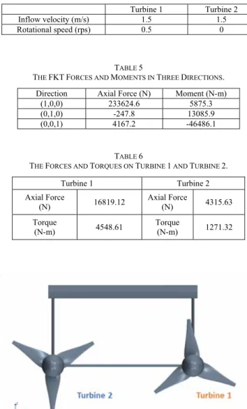
TABLE 4

CONDITIONS FOR ONE SIDE MALFUNCTION SIMULATION . Turbine 1 Turbine 2

Inflow velocity (m/s) 1.5 1.5

Rotational speed (rps) 0.5 0

TABLE 5

THE FKTFORCES AND MOMENTS IN THREE DIRECTIONS. Direction Axial Force (N) Moment (N-m)

(1,0,0) 233624.6 5875.3

(0,1,0) -247.8 13085.9

(0,0,1) 4167.2 -46486.1

TABLE 6

THE FORCES AND TORQUES ON TURBINE 1 AND TURBINE 2.

Turbine 1 Turbine 2

Axial Force

(N) 16819.12 Axial Force

(N) 4315.63

Torque

(N-m) 4548.61 Torque

(N-m) 1271.32

Fig.11 The relative position between turbine 1 and turbine 2. The perspective is downstream of the FKT turbine.

Fig. 12 The flow filed of one side malfunction situation

To simulate one turbine breaks down, the setting of inlet conditions and turbine operating conditions are showed in Table 4, and Fig. 19 illustrates the relative position between Turbine 1 and Turbine 2. The perspective is downstream of the FKT turbine. In this simulation, Turbine 1 (the right one) keeps a rotational speed of 0.5 rps, and Turbine 2 (the left one) is stationary. The inlet velocity is 1.5 m/s for both turbines.

Table 5 are the results obtained from the RANS computations, and it shows the axial forces and moments on FKT in three directions, and Since the analysis assumes that the center of mass is at (0,0,0) position, namely, the two turbines lie on the same line, the force caused by the floating body leads to y- direction torque (pitch). In the actual situation, the center of mass should be in more forward position, so that the arm is reduced and the torque is also reduced. Because only one side turbine operates, the forces on FKT are not stable, which brings on the torque in other direction. Table 6 shows the axial forces and torques on Turbine 1 and Turbine 2 respectively.

Fig. 12 shows the flow filed of one side malfunction situation. Because on turbine breaks down, the forces and torques on two turbines cannot be cancelled, and the uneven forces and the torques from different directions cause instability of the FKT. Based on the analysis above, the FKT might rotate irregularly or even overturn in the ocean when this situation takes place.

IV. S^TRUCTUREA^NALYSISR^ESULT

In addition to the above analysis of hydrodynamic performance, FKT structure analysis is discussed in this section. The FKT turbine will be placed in the ocean and must operate in the Kuroshio for a long time, its structure not only needs to resist dynamic pressure and hydrostatic pressure by fluid but also meets the rule requirements after considered the safety factor. FRP is used as material of the blade, and the structure strength is analysed by the finite element method (FEM). We applied Tsai-Wu Index and maximum stress criterion to evaluate whether the fibre of each layer of FRP reaches destruction or not. The strength of core material was examined by Von Mises stress and Principal stress. The parameters obtained by above analysis methods are then checked against the BV and DNVGL regulations.

(6)

Fig. 13 The relationship between inflow and the FKT in FEM analysis.

Fig. 14 The FRP sandwich structure, and blade is divided into suction side and pressure side.

The blade structure was analyzed by static loading simulation, and Fig. 13 illustrates the relationship between inflow and FKT in FEM analysis. The FRP structure is shown in Fig. 14, and blade is divided into suction side and pressure side. FRP is a sandwich structure (as shown in Fig. 14), the inside part is the core material and the outside part is FRP. We applied hydrodynamic pressure and hydrostatic load of 50m design depth to the blade surface for FEM analysis and overall deformation, the Tsai-Wu values of fiber in each layer of FRP, the stress values parallel to the fiber direction_σ_{/ / fiber}, the stress values vertical to the fiber direction σ⊥fiber, sheer stress τfiber , and the Von Mises stress, and Principal stress of the core are computed.

TABLE 7

THE RESULTS OF STRUCTURE ANALYSIS.

Variable

Dynamic + Hydrostatic

Critical area σ / σ_permissible

DNVGL BV

FRP

σ//fibre 0.16 0.32 Ply24 L900

0°

σ┴fibre 0.90 0.85 Ply27 DBLT1800

90°

τfibre 0.37 0.58 Ply28 DBLT1800

-45°

Tsai-Wu 0.39 0.56 Ply28 DBLT1800

-45°

Core

VM Stress 0.20 0.21 Tip

Principal

Stress 0.47 0.53 Tip

Global U 72.77mm Tip

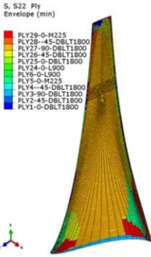
Fig. 15 The stress distribution of the 27^th layer fibre (DBLT1800 90°).

Fig. 16 The deformation at the tip of the blade is 72.77mm, which is about 3.83% relative to the blade length.

Table 7 shows the results of structure analysis, and all parameters are displayed in the way that the stress divided by permissible stress. If the number is smaller then 1, it means that structure strength meets the regulation. Although the values of Tsai-Wu, _σ_⊥_fiber and _τ_fiber are all smaller than regulation requirements, the _σ_⊥_fiber of the 27^th layer fibre (DBLT1800 90°) is quite close to the allowable stress. Fig. 15 shows that stress distribution of the 27^th layer fibre (DBLT1800 90°), it can be observed that the area close to the allowable stress value is not small. The reason is that DBLT1800 is a unidirectional material, and its strength in the second direction is weak. It may be beyond the specification if the forces are slightly changed. To improve this problem, we can increase the strength of the blade in the direction of fibre length which is 0^ unidirectional material. Table 7 also shows the strength analysis of the core material. The Von Mises stress and Principal stress are all less than the allowable stress,

(7)

and it indicates that the strength of the core material is sufficient. Fig. 16 shows the deformation at the tip of the blade, and it is 72.77mm, about 3.83% relative to the blade length.

V. CONCLUSIONS

In this paper, the design procedures of a FKT are briefly introduced, and the performances of designed geometry are computed by both potential flow BEM and viscous flow RANS method. The computational results are also compared to the experimental data. All the results confirmed that the designed FKT geometry achieved the design goal. In addition to the analysis of the blade geometry, the overall FKT performances were also analysed, and results show that no significant influence on performances with the floating body.

We also simulate the situation that the turbines have one side malfunction. The two turbines are unbalanced and then lead to the overall FKT might be in irregular rotations in the current.

In terms of structure strength, we investigate whether FRP materials can withstand long-term stress in ocean current by FEM. Overall strength of FKT structure are sufficient.

However, because of the unidirectional materials, some FRP layers might be in critical condition according to the rule requirements. To prevent the structure damages, the material should be strengthened in other directions.

ACKNOWLEDGMENTS

This research project is funded by the Ministry of Science and Technology under National Energy Program, Phase II, Taiwan, R.O.C., MOST 104-3113-E-002-020- CC2. The experiment in this paper is carried out by Professor Tsai Jing- Fa at National Taiwan University.

The authors would like to thank for his support.

REFERENCES

[1] C.-Y. Hsin, Efficient Computational Methods for Multi-component Lifting Line Calculations, M.S. Thesis, MIT, Cambridge, MA, USA (1986).

[2] J.E. Kerwin, W.B. Coney and C.-Y. Hsin, “Optimum circulation distributions for single and multi-component propulsors,” 21st ATTC Conference, Washington, DC, USA (1986).

[3] D.S. Greeley and J.E. Kerwin, “Numerical methods for propeller design and analysis in steady flow,” SNAME Trans., Vol. 90, pp. 415- 453 (1982).

[4] Y.-S. Luo, Investigation of the Current Turbine Performance by Computational Methods, M.S. Thesis, National Taiwan Ocean University, Keelung, Taiwan (2013).

[5] S.-Y. Wang, Improvement of Marine Current Turbine Blade Design by Using the Genetic Algorithm, M.S. Thesis, National Taiwan Ocean University, Keelung, Taiwan (2015).

[6] C.-Y. Hsin, S.-Y. Wang, J.-H. Chen and F.-C. Chiu, “Design of Floating Kuroshio Turbine Blade Geometries”, Journal of Taiwan Society of Naval Architects and Marine Engineers, Vol. 35, No. 3, pp.145-153, 2016

[7] C.-Y. Hsin, S.-Y. Wang, J.-H. Chen and F.-C. Chiu, “Design of Floating Kuroshio Turbine Blade Geometries”, 3rd Asian Wave and Tidal Energy Conference (AWTEC2016), Oct. 24-28, 2016, Singapore