MAXIMUM BITRATE-LENGTH PRODUCT IN THE HIGH-DENSITY WDM OPTICAL FIBER COMMUNICATION-SYSTEM

(1)

deviation of parameter variations, AJ is chosen to be suffi- ciently large.

In order to check the stability of the discrete TVCNF,, its difference equation was solved by a sequential procedure using a digital computer for a = 0.999 andf, = 0.1. The fre- quency F was increased from F = IO-’ up to F =fo = 0.1. For each F the values of Aj for which the system becomes unstable was found. Fig. 1 shows the results obtained. There exist unstable regions represented by shaded zones. It is seen that in order to get oscillations for low F a large Afis needed. Such a relationship between F and Af also follows from the analysis of the Mathieu equation3 as well as the fact that there exist such frequencies F for which the system is stable even for large A$

Filter with t w o controlled coefficients-TVCNF,: As shown in Reference 4, to reject any sine signal with a time varying frequency, given by A cos [ ( ~ ( k )

+

91,

the two coefficients of TVCNF, have to be functions of the instantaneous phase ~ ( k )

with 0 < $ ( k - 1) - + ( k - 2) < II as we are dealing with posi- tive frequency less than II.

Our goal is to check whether TVCNF, described by eqn. 1 and having the coefficients given by eqn. 4 is asymptotically stable, i.e., to check if the output response of the unforced system (AR part of eqn. 1) approaches zero as k + 00, far any arbitrary initial conditions. For that purpose let us consider an exponentially damped FM signal

y(k) = Aa(k-’o’ cos [ $ ( k )

+

91

k > ko ( 5 ) It can be proved by constructing an augmented Casarati’s determinant associated with y(k), that all independent solu- tions of the difference eqn. 1 with coefficients given by eqn. 4 may be derived from eqn. 5. The values of A and

4

in eqn. 5 depend on the initial conditions y(ko - 2) and y(ko - I). It follows from eqn. 5 that y ( k ) + 0 for k + CO for any A and

4,

and therefore for any initial conditions, i.e., the system is asymptotically stable. It is interesting to see that TVCNF, even though is a stable system may have ‘poles’ lying outside the unit circle. This is not surprising since the concept of poles, developed for time-invariant systems, can not be generally applied to time-varying systems.

139312/ Fig. 2 Asymptotic stability area and stability triangle

Consider a structural relationship between a,(k) and a,(k)

a , ( k ) = -cos [ $ ( k ) - $(k - 1)l which follows from eqn. 4

+

cos

C

W

- 1) -

W

-

211&),

a,W) > 0 (6)

From eqn. 6 the structural constraines are obtained

I a , ( k )

I

I 1

+

4 )

> 0 (7) The conditions of eqn. 7 are sufficient conditions for asymptotic stability and may be represented by the asymptotic stability area-the area between two semi-infinite lines which start at-points D and G respectively and the axis a,, as shown in Fig. 2. A stability triangle ABC,5 which determines the stability of time-invariant system, is also shown for compari- son purposes. As expected, the asymptotic stability area and the stability triangle overlap but do not coincide.

Conclusion: Stability of second order TVCNFs, which are capable of rejecting a sine signal with time-varying frequency, was analysed. If the coefficients a&) and a&) of TVCNF, are found as functions of the instantaneous phase of the sine signal, then using the relationships between them it is proved that TVCNF, is asymptotically stable. On the other hand, it is shown that the AR-part of TVCNF, can be explicitly described by the Mathieu equation and therefore such a lilter possesses unstable regions, i.e., becomes generally unstable. This fact explains why, for processing a sine signal with time varying frequency (FM), CANF with two controlled coefficients is always preferable to a CANF having only one coefi- cient.

D. WULICH

E. I. PLOTKIN

M. N. S. SWAMY

17th May 1990

Department of Electrical and Computer Engineering, Concordia University,

1455 DeMaisonneuue Blud., Montreal, Quebec H3G I M 8 , Conado

References

1 RAO, D. v. EL, and KUNG, s. Y.: ‘Adaptive notch filtering for the retrieval of sinusoids in noise’, IEEE Tram., 1984, ASP-32, pp.

791-802

2 NEHORAI, A.: ‘A minimum parameter adaptive notch filter with

constrained poles and zeros’, IEEE Trans., 1985, ASP-33, pp.

983-996

3 RICHARD$ I. A.: ‘Modeling parametric processes-a tutorial review’, Proc. IEEE, 1977.65, pp. 154%1557

4 WULICH, D., PLOTKIN, E. I., and SWAMY, M. N. s.: ‘Synthesis of discrete time varying null filters for frequency varying signals using the time warping technique’, IEEE Trans., 1990, CAS-37, (to be published).

5 SHYNK, I. I.: ‘Adaptive IIR filtering’, IEEE ASSP Magazine, 1989,

pp. 6 2 1

M A X I M U M BITRATE-LENGTH PRODUCT I N THE HIGH DENSITY W D M OPTICAL FIBRE C O M M U NI CATION SYSTEM

Indexina Ootical communications. Raman scatterina

The bitrate-length product in the high density WDM optical fibre communication system is analysed by numerical simulation in which both dispersion and Raman crosstalk are wn- sidered, and the maximum bitrate-length product is obtained under certain constraints.

In a wavelength division multiplexed (WDM) optical fibre communication system, the bitrate-length product NBL ( N : channel number, B : bitrate for a single channel, L: propagation length) measures the capacity of the systems. In this letter we use computer simulation to find the maximum NBL

product under certain constraints.

1509 ELECTRONICS LETTERS 30th August 1990 Vol. 26 No. 18

(2)

In the analysis, we do not consider any nonlinear effects except Raman crosstalk between channels. In order to get the maximum NBL value, dispersion-shift fibre is used whose zero dispersion wavelength 1, is shifted to 1.55pm. The loss coeffi- cient is assumed to be constant. Here we also assume that the polarisation of the fibre is maintained and the laser source is monochromatic.

The differential equations governing the signal propagation are given by1.'

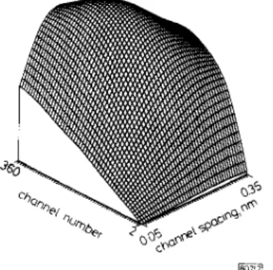
Since the channel of the shortest wavelength (the first channel) is degraded most severely by the Raman crosstalk, and the dispersion curve is hearly symmetry in the zero dispersion region, the first channel determines both the bitrate and the propagation length. The signal pulses are assumed to be of Gaussian form with constant energy. For a given channel number, N, and channel spacing, AA, eqn. 1 is solved by the split-step Fourier method. Then the maximum propagation length can be obtained by checking the propagation length of the first channel. The maximum NBL product is obtained by using eqns. 2 and 3. Plotting these maximum N B L values as a function of N and A1 in Fig. 2, we can find an overall

-

where the subscript i = 1, 2, . . . , N denotes the ith channel, and v. I , A are the group velocity, wavelength and slowly varying amplitude of the electric field intensity, respectively, and are the first and second order dispersion coefficients.

gl, is the Raman gain constant coupling the ith and jth channels, c( is the loss constant and A , is the effective core area

In our analysis, we assume a = 0.18dB/km and A,, = 6.36

x 10-"m2. We also assume that I , < I , ,

...,

<

L,

and the N channels are placed symmetrically at the both side of 1, with equal channel spacing A I . In order to calculate gi, we use a near triangle function (solid curve in Fig. 1) to approximate

0 200 400 600 800 freqwncyshift c 6 '

h?L Fig. 1 Measured andfitted Raman gain profile

. . . measured curve fitted curve _ _

the actual Raman gain profile of silica (dashed curve in Fig. I), i.e., the peak Raman gain, go, occurs at 440 cm-'. For the frequency separation larger than 500 cm-' the Raman gain curve drops as an exponential decay function.

Several criterion are used in our analysis to set up the system model. The minimum detectable energy at the output end is lo4 photons' (about 1.3 x lo-" Joules). When the channel spacing AA is larger than the modulation spectrum width of the signal pulse, the minimum output pulse width for a fixed L is obtained by differentiating the following equation4 with respect to ui:

where U and U, are the root mean square width at the output and input end, respectively. When AI is smaller than the modulation spectrum, the above formula will no longer be useful, because the modulation spectrums of two neighbouring channels must be resolvable in the frequency domain. Here we take A1 (nm) as four times of the root-mean-square width of the modulation spectrum (g 2.55/u,, ui in picoseconds). The largest bitrate B to guarantee a clear detection in the time domain is given by'

1

B = -

4u (3)

1510

Fig. 2 Three dimensional diagram oJNBL product

maximum N B L product. In our example, pulses with lo-'' joule (about several milliwatt in peak power) are launched, and the maximum value is found to be 3.27 x 10' km Gbit/s at N = 240 and A1 = 0.2 nm. It is noticeable that the 3D surface in Fig. 2 composes of infinite 2D curves, and each curve has a local maximum point either for a fixed N (Fig. 3) or for a fixed

005 015 025 035 channei spacing AA nm

rn

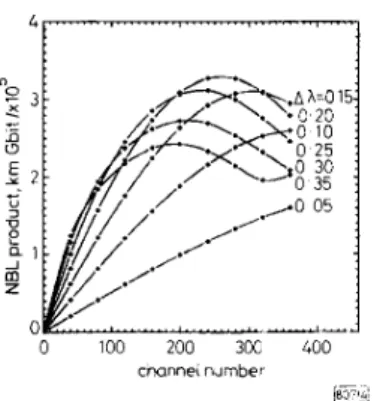
Fig. 3 N B L product against channel spacing for various channel number

AI (Fig. 4). The reason for the existence of these local maximum values is that for a fixed channel number, larger AI induces more Raman crosstalk and dispersion and conse- quently decreases the N B L product. For smaller AI the N B L curve crops owing to the limitation of modulation spec- trum. On the other side, for fixed AA, larger N induces more Raman crosstalk and dispersion and hence reduces the NBL product, when N is small this degrading effect is not evident and is less than the increasing rate of N, the NBL product increases as N increases.

It was also found that if we change the launching energy and repeat the same procedure we will obtain a set of 3D surfaces as in Fig. 2. The maximum NBL product of each surface changes as the launching energy changes and we can get a optimum launching energy for the NBL product. In summary, if we fix any two of the parameters channel number, channel spacing, and launching energy we can obtain a concave down curve as in Fig. 3 or Fig. 4. This conclusion is applicable not only for the constant loss assumption but is ELECTRONICS LETTERS 30th August 1990 Vol. 26 No. 18

(3)

also applicable for the wavelength dependent loss. The difference between these two cases is that the N B L curve goes

0 100 200 3cc 400

channel number

@I%

Fig. 4 N B L product against channel number for various channel

spacing

sharper in the latter one and the position of zero dispersion wavelength 1, will play an important role.

S. CHI 17th July I990

S.-C. WANG

Institute of Electro-Optical Engineering and Centre for Telecommunica- tions Research,

National Chiao Tung University, Hsinchu, Taiwan, Republic of China

References

I AGRAWAL, G. P.: ‘Nonlinear fibre optics’. (Academic Press, New York, 1989), pp. 21&228

2 KAo, M. s., and w, J. s.: ‘Signal light amplification by stimulated Raman scattering in an N-channel WDM optical fibre communication system’, J . Lightwoue Technol., 1989, LT-7, pp. 129C-1299 3 OGTKOWSKY, D. E., and SPITZ, E. (Ed.): ‘New directions in guided

wave and coherent optics’. (Martinus Nijhoff, 1984), pp. 43-60 4 MARCUSE, D.: ‘Pulse distortion in single-mode fibers’, Appl. Opt., 19,

pp. 1653-1660

5 NEUMANN, E. G.: ‘Single-mode fibers’ (Springer-Verlag, 1988). pp.

256264

UNIFIED APPROACH TO ANALYSE MASS SENSITIVITIES OF ACOUSTIC GRAVIMETRIC SENSORS

Indexing terms: Acoustic transducers, Sensitivity

A unified approach based on Rayleigh’s hypothesis for evalu- ating the mass sensitivities, S,, of bulk, surface, plate and thin rod flexural acoustic gravimetric sensors is presented. The estimation of S, uses the ‘equivalent depth’ which is determined by the displacement distribution of the acoustic mode. The S,’s for the lowest order torsional and longitudinal mode of a thin rod are reported for the first time.

Introduction: Research and development In the area of inte- grated acoustic gravimetric sensors based on bulk (BAW),’ surface (SAW),’ plate’ and thin rod4 flexural acoustic waves has become of increasing interest. In order to have high accu- racy and sensitivity, these acoustic sensing devices normally operate in the single mode regime. Thus, the BAW of a bulk material,’ the SAW of a semi-infinite substrate,’ the lowest antisymmetric Lamb, A0,3.5 and shear horizontal, SH0,5,6 modes of a thin plate, and the lowest order longitudinal, Lo,,’ torsional, and flexural, F1,,4.5 acoustic modes of a thin rod, which can be excited and received predominantly in a single mode regime, are of interest.

For acoustic gravimetric sensors the oscillator mode is often used.’-3 With this method, an acoustic resonator is used

as the frequency control element for the oscillator circuit. A perturbation in the oscillator frequency is monitored in response to changes caused by the measurands. Using Ray- leigh’s hypothesis, Lu’ analysed the dependence of the bulk wave resonator frequency on the mass loading. Martin et al.: also used this hypothesis to analyse mass sensitivities S,’s of the gravimetric sensors comprised of SH mode plate wave resonators. In this letter, Rayleigh’s hypothesis is further extended to analyse the S,’s of SAW,’.’ thin plate flexural A , acoustic3 and thin rod F,,,4 To, and Lo, devices.

Rayleigh hypothesis approach: According to Rayleigh’s a mechanical resonant system oscillates at a fre- quency at which the peak kinetic energy U, is equal to the peak potential energy U, in the same volume. The energy that appears as a potential energy at a particular time must be totally converted into a kinetic energy after a quarter cycle. For acoustic gravimetric sensors, if the loaded mass layer is very thin and does not contribute to the elastic property of the resonator, the added mass layer will not store any potential energy during the vibration cycle. The peak kinetic energy of the perturbed system will therefore remain unchanged for the unperturbed resonator. ‘ A

The kinetic energy of a mechanical resonator can be expressed by

V

where o, = 2rrl; and

1;

is the resonant frequency, p is the density of the vibrator material, uXxz) is the displacement of the component polarised in the xi direction at a position xz, and V is the volume of the mechanical resonator. Later in the text, xl, x2 and x, refer to Cartesian X, Y and Z axes or cylindrical R ,

6

and Z axes. The analysis here is restricted to two dimensional structures. We assume that the acoustic field distribution is independent of x for the rectangular structures, and that it is azimuthally symmetric for the rod structures.

For the sake of simplicity, the modes with only one displacement component will be discussed. We further assume the y

direction to be the propagation direction for bulk waves and the z direction for othep wave modes. Based on eqn. 1 the kinetic energy density per unit area on the principal plane for the rectangular structures is

0

where d is the depth of the acoustic energy distribution in the substrate. For SAW devices the integration limit, d, can be replaced by a few wavelengths. The kinetic energy density per

unit length for the rod structures can be expressed as

U , = ( 2 4 I u(r) I’r dr

2

0

where a is the radius of the rod and u(y) or u(r) is the displacement distribution of the corresponding mode.

When a mass layer is deposited on the surface of the resonator, and if the loaded layer is very thin so that the mass loading does not alter the distribution of the acoustic fields in the resonator, the kinetic energy density of the perturbed resonator can be expressed by

d

0

for the rectangular structures and

ELECTRONICS LETTERS 30th August 1990 Vol 26 No 18