A polynomial-perceptron based decision feedback equalizer with a robust learning algorithm

(1)

Signal Processing 47 (1995) 145-158

A polynomial-perceptron

based decision feedback equalizer with

a robust learning algorithm

Ching-Haur Chang”, Sammy Siub, Che-Ho We?*

a Institute of Electronics, Nafional Chiao-Tung University, Hsin Chu, Taiwan 300, ROC

b Telecommunication Laboratories, MOTC, P.O. Box 71, Chung Li, Taiwan 320, ROC

Received 3 December 1993; revised 1 July 1994, 10 January 1995 and 27 July 1995

Abstract

A new equalization scheme, including a decision feedback equalizer (DFE) equipped with polynomial-perceptron model of nonlinearities and a robust learning algorithm using lp-norm error criterion with p < 2, is presented in this paper. This equalizer exerts the benefit of using a DFE and achieves the required nonlinearities in a single-layer net. This makes it easier to train by a stochastic gradient algorithm in comparison with a multi-layer net. The algorithm is robust to aberrant noise for the addressed equalizer and, hence, converges much faster in comparison with the /,-norm. A detailed performance analysis considering possible numerical problem for p < 1 is given in this paper. Computer simulations show that the scheme has faster convergence rate and satisfactory bit error rate (BER) performance. It also shows that the new equalizer is capable of approaching the performance achieved by a minimum BER equalizer.

Ein neues Entzerrungsverfahren wird in diesem Beitrag vorgestellt. Es schlief3t einen Entzerrer mit Entscheidungsriick- fiihrung ein, der mit einem Polynom-Perceptronmodell fiir Nichtlinearitlten und einem robusten Lernalgorithmus ausgestattet ist, welcher mit einem I,,-Norm-Kriterium mit p < 2 arbeitet. Dieser Entzerrer nutzt den Vorteil der Entscheidungsriickkopplung und erzielt die gewiinschten Nichtlinearitgten in einem Netzwerk mit einer Ebene. Gegeniiber einem mehrlagigen Netzwerk wird so das Training durch ein stochastisches Gradientenverfahren erleichtert. Der Algorithmus ist beim angesprochenen Entzerrer robust gegeniiber Fehlerrauschen und konvergiert daher vie1 schneller als bei Verwendung der I,-Norm. Die Leistungsftihigkeit wird beziiglich maglicher numerischer Probleme fiir p < 1 im einzelnen analysiert. Rechnersimulationen zeigen die h&here Konvergenzgeschwindigkeit und zufriedenstel- lende Bitfehlerrate. Es zeigt sich aul3erdem, daLi der neue Entzerrer fihig ist, die Leistungsfihigkeit einer Entzerrung mit minimierter Bitfehlerrate zu erreichen.

Cet article prksente un nouveau schCma d’6galisation incluant un Bqualiseur g decision par retour arri&e (DFE) Cquip6 avec une mod6lisation des non-Marit& par modkle de perceptron polynomial et un algorithme d’apprentissage robuste utilisant la norme I, comme crit&e d’erreur (avec p < 2). Cet ggaliseur exploite les avantages d’une DFE et remplit les conditions de non-1inCaritC requisent par un rkseau monocouche. Ce dernier point permet un

*Corresponding author.

(2)

146 C-H. Chang et al. /Signal Processing 47 (1995) 145-158

apprentissage par un algorithme de gradient stochastique plus facile par comparaison g un rCseau multi-couche. L’algorithmeest robuste au bruit aberrant dans le cas de l’bqualiseur utilisk, et, de plus, il converge plus rapidement que la norme Iz. Une analyse dCtaillCe des performances tenant compte des problkmes numkiques lorsque p < 1 est don&e dans cet article. Les risultats de simulation montrent que le schCma a une vitesse de convergence plus rapide et des performances en terme de taux d’erreur par bit satisfaisant. 11 montre Cgalement que ce nouvel Cgaliseur est capable d’approcher les performances d’un tgaliseur a BER minimum.

Keywords: Robust learning algorithm; Polynomial-perceptron based DFE; l,-norm error criterion

1. Introduction

Adaptive equalization is an important technique to combat intersymbol interference (ISI) in digital communication systems. The equalizer has the task to recover the transmitted sequences from the received signal. It is well understood that optimal performance can be obtained by detecting the entire transmitted sequence using the maximum likelihood sequence estimator (MLSE) [7, 151. However, the computation complexity and memory requirement of the MLSE make it impractical in some real-time applications. A more practical approach is to use symbol-by-symbol-decision linear transversal equalizer. However, it is known that in the signal space only linear decision boundaries [14] can be formed by a linear equalizer. An opti-

mal symbol-by-symbol-decision equalizer must

realize some nonlinear functions such that it can partition the signal space with nonlinear decision boundaries [4, 5, 91. Recently, nonlinear equalizers

equipped with multi-layer perceptron (MLP)

model of nonlinearities were proposed by Gibson et al. [9] and Siu et al. [23]. Their results indicated that the optimal decision boundaries must be nonlinear and the MLP can approach the required nonlinearities. In addition, nonlinear approaches equipped with different models of nonlinearities such as using a polynomial-perceptron structure (PPS) [4], a radial basis function [S] and using a functional-link net [S] were demonstrated to have similar capabilities in partitioning the signal space.

In this paper, we focus on a new nonlinear equalizer in the following two respects. First, a single-layer nonlinear decision feedback equalizer

(DFE) equipped with polynomial-perceptron

model of nonlinearities is developed, Second, an

&-norm [21] based learning algorithm suitable for the addressed structure is investigated. The structure exerts the benefit of using a DFE and achieves the required nonlinearities in a single-layer net. This is advantageous since it is much easier to train by a stochastic gradient algorithm. The algorithm using /,-norm error criterion with p < 2 can be robust to aberrant noise when the distribution of error signals is more or less known a priori. The new equalizer has error signals lying in an interval suitable for applying the l,-norm error criterion. A performance analysis of the l,-norm back propagation (BP) algorithm [ZO] with p > 1 has been conducted by Siu et al. [22] for an MLP equalizer. A detailed performance analysis with a consideration on the possible numerical problem arising when p < 1 is given in this paper. Computer simulations show that the new equalizer is attractive in both convergence rate and BER performance and has a performance close to that achieved by a minimum BER equalizer.

The paper is organized as follows. Section 2 de- scribes the polynomial-perceptron based DFE. Sec- tion 3 presents the [,-norm tap-weight updating algorithm for the proposed structure. A performance analysis of the l,-norm algorithm with a numerical stability consideration is given in Section 4. Computer simulation results are given in Section 5. A comparison of the new equalizer with other nonlinear equalizers is given in Section 6.

2. Polynomial-perceptron based DFE

The capability of a single-layer net is limited since only linear decision boundaries can be formed in the pattern space [16]. Although the use of

(3)

C.-H. Chang et al. /Signal Processing 47 (1995) 145-158 141

a multi-layer net [20, 241 can achieve the required nonlinearities, the high complexity of the multi- layer net precludes its use in many applications. It is known that functions realized by hidden layer nodes in a multi-layer net can also be realized or approximated by a single-layer net provided that sufficient orders of nonlinear links are incorporated into the node [17]. For example, consider a set of components described by a vector X1, the required nonlinearities can be achieved by a series of higher- order expansion as

XI +X2 =

[XII x t-1, XII

-+X,=[X,]x[l,X,]+ . ..) (I)

where x denotes outer product operation. This expansion introduces higher-order terms, together with the first-order terms given by X1, to represent the information. Some advantages through the use of the outer product model can be found in [17]. A perceptron with nonlinear links obtained by using (1) on the input is called a polynomial perceptron [4].

Let L and M denote, respectively, the number of taps in the feedforward and the feedback filters of a DFE. The signal vector in a DFE can be represented as

T

X(n) = [X,(n),

X,(41 I

with

(2)

X,(n) = [x&r), xr(n - I), ... ,x&r - L + l)], (3) X,(n) = [x&i - I), x&i - 2), 1.. ,x&i - Ml, (4) where X,(n) and X,(n) denote, respectively, the feedforward and the feedback signal vectors. In a DFE, the feedforward and feedback signals can be highly correlated [2]. This fact can be seen from the cross- correlation between X,(n) and X,(n) given as

Notice that the elements in (4) are related to the equalizer delay d by

x&r) = s(n - d) + v(n), (6)

where s(n) is the transmitted signal and v(n) is the decision error. Moreover, it is reasonable to assume that the decision error is independent of the feedforward signal. Consequently, the elements in (5) become

E[x& - i)xb(n -j)] = E[xf(n - i)s(n - d -j)],

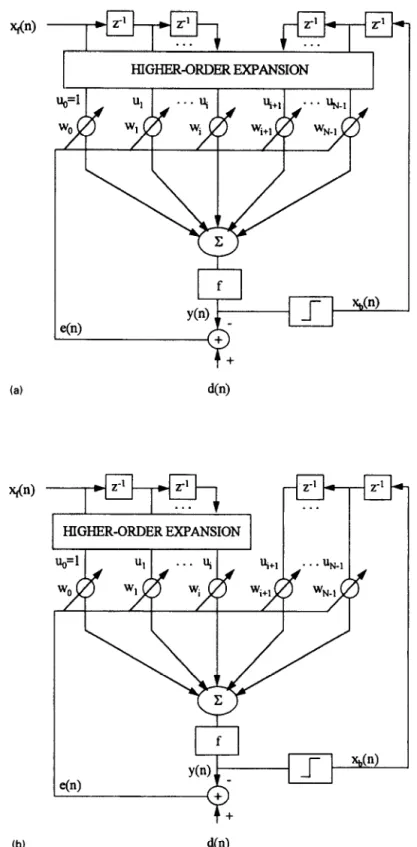
(7) with i = 0, 1, . . . ,L-landj=1,2 ,..., M.Wecan see from (7) that the elements in (5) depend solely on the channel response. The polynomial-perceptron based DFE shown in Fig. l(a) is denoted as PPDFE-I, where the threshold term for the perceptron is treated as an input of value unity (ue = 1) with tap-weight W&I). The DFE shown in Fig. l(b), denoted as PPDFE-II, uses the same higher-order expansion but only on the feedforward part of X(n). The number of taps needed for an ith-order expansion can be found by

N= i nk,

(8)

k=O

with no = 1 and nk = nk_ 1(L + M + k - 1)/k, k = 1,2, . . . , i [4], for PPDFE-I, while

1

N = 1 nk -t M,

k=O

(9)

with no = 1 and nk = n,_,(L + k - 1)/k,

k = 1,2, . . . . i, for PPDFE-II. Given the same L and M, the number of taps in PPDFE-I is larger than that of the PPDFE-II for a given order of expansion. For example, if L + M = 5 and i = 3, the PPDFE-I has 56 taps, while the PPDFE-II has

E CX~(n)Xdn)l

xf(n)xb(n - 2) ...

xf(n - 1)x& - 1) xf(n - l)x+,(n - 2) ‘..

= E xf(n - l)xb(n - M) _. ₍₅₎

(4)

148 C.-H. Chang et al. /Signal Processing 47 (1995) 145-158

I

HIGHER-ORDER EXPANSION

(a)

1 HIGHER-ORDEREXF’ANSION 1 )

(b) d(n)

(5)

C-H. Chang et al. /Signal Processing 47 (1995) I45- I58 149

36 taps. This is the price paid by the PPDFE-I for its better performance. The number of taps grows exponentially with increasing order of expansion. However, a small order such as 3 or 5 is often adequate to achieve required nonlinearities encountered in practical applications [4]. Further- more, higher-order terms for which the correlation is insignificant can be dropped. This makes the proposed structure more feasible.

3. l,-norm learning algorithm

The lack of robustness in the least-mean square (LMS) algorithm is attributed to its overweighing of aberrant noise in the error signal. Therefore, for the LMS algorithm to be robust, an appropriate error suppressor must be equipped prior to evaluating the increments of the tap-weights. For example, a robust LMS algorithm can be of the form W(n + 1) = W(n) +

~zc.(n)l~,

where q is the learning gain and z( .) is an error suppressor. If, for example, the error signal has a probability density function (PDF) that re- sembles a logistic density, then a function of the form z[e(n)] = tanh[e(n)/2] can be a robust error suppressor [13]. However, the PDF of an error signal is generally not known a priori and hence the determination of an error suppressor is subject to trial and error. An alternative way to achieve this goal is to use the I,-norm error criterion with p < 2. The l,-norm error function [21] is defined by

(11)

where p denotes the power metric and the factor of P - ’ is padded simply for mathematical conveni- ence [17, 203. For p = 2, (11) becomes the mean squared error (MSE) or the &-norm error criterion. Similar to the rule of LMS algorithm, the negative gradient, - VP(n), in the p-power error surface can be estimated as

-

V,(n) = ) e(n)lPml _-

Wn)

_{sfzn Ce(n)l,}

aw(n)

(12)

where sgn[e(n)] denotes a sign function of e(n). We can see from (12) that a nonlinear error function of the form

4441 = sgn Ce(4lI44 Ip- ’ (13)

is now inherently built in the tap-weight updating equation.

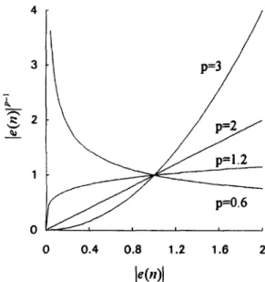
The factor I e(n) Ip- ’ in (13) rescales I e(n) I to some extent if p # 2. Fig. 2 shows how 1 e(n) 1 is resealed by I e(n) Ip- ’ using different values of p. The value of

le(n)l is assumed to be in the interval [0,2]. For p > 2, I e(n) Ip- ’ scales up large values of I e(n) I and scales down small values of I e(n) I. This tells why the use of p > 2 cannot be robust when possible statistical outliers [lo, 121 are located close to the upper bound of le(n)l. For p c 2, I e(n) Ip- ’ scales down large values of le(n)l and scales up small values of le(n)l to some extent. This indicates that the use of p < 2 can provide a robust error suppressor if possible statistical outliers are located close to the upper bound of I e(n)I. However, for p < 1, a numerical stability problem arises whenever

(e(n) 1 is close to zero. This is the issue that must be resolved when using p < 1. Notice that using I,- norm with p < 2 could throw some information away if the distribution of le(n)l is not known completely.

lwl

(6)

150 C.-H. Chang et al. /Signal Processing 47 (1995) i45- 158

The tap-weight updating equation for the proposed DFE is derived as follows, The equalizer output y(n) in Fig. 1 can be written as

y(n) =.fCwT(GJ(n) +

WOWI,

(14)

where f( .) is the activation function, we(n) is the threshold level for the perceptron, W(n) = [wr(n), W&r), ... , wN_ l(n)]T is the tap-weight vector, and U(n) = C% (n), u2(4, . . . , UN_ 1(n)]’ is the input vec-

tor comprising components to be supplied to the perceptron. If the activation function is of the form f(x) = (1 - e-“)/(l + e-“), then the resulting tap- weight and threshold level updating equations can be written, respectively, as

lV(n + 1) = W(n) + v] sgn [e(n)] 1 e(n)]“- ‘f’(n) U(n), (15) wo(n + 1) = we(n) + P

wC441 I 441p- Y’W,

(16)

where fl is the threshold level adaptation gain and f’(n) is the derivative of the activation function

with respect to its argument, that is, f’(n) = [l - y2(n)]/2. It can be seen from (15) or (16) that the 12-norm yields a standard LMS algorithm and the Ir-norm yields a sign algorithm. Table look-up method can be employed to implement the factor 1 e(n) Ip- ’ in the algorithm.

4. Performance analysis of the I,-norm algorithm The following analyses will focus on the tap- weight updating equation given by (15) since the same results can be applied directly to the threshold level update. To see the effect of p on the learning

gain, we rewrite (15) as

W(n+l)=W(n)+ V

14n)12-P s(n) U(n), (17)

where z(n) F e(n)f’(n) is the change of error at

p = 2 and q is the learning gain at p = 2. Having

this, the effective learning gain at arbitrary values of

p can be written as u,(n) = q/l e(n)12-P. Further

investigation of this requires a priori knowledge of 1 e(n)l. For the assumed activation function f, the

output will be limited by the interval [ - 1, 1) and most of it will be located close to its steady states, - 1 or 1 in our case, due to the nonlinearities off: If the desired signal has an alphabet of (- 1, l}, then I e(n) I will be distributed in [0,2] and most of them will be located close to its lower bound under correct decisions. Consequently, using I,-norm with

p < 2 can treat I e(n) I in a ‘robust’ manner as dis- cussed in the last section. Without loss of general- ity, the output is assumed to be uniformly distributed in [ - 1, l] for simplicity [19] in the following analyses. Having this, 1 e(n) I will be uniformly distributed in [O, 21.

4.1. lp-norm for p < 1

The possible numerical problem encountered when using p < 1 can be solved by replacing (e(n) I with a small positive number 8 whenever I e(n) 1 d 8.

Although alternative method, such as switching

p from p< 1 to p b 1 when [e(n)1 < 8, could be

feasible, only the former is focused in this paper. The following results are valid if 1 e(n) I is bounded in the interval [0,2] and 8 is limited by 8 < 1.

In the training mode, a correct decision makes

le(n)l to be distributed in [e, 11, whereas an incor- rect decision makes I e(n)1 to the distributed in [1,2]. Let P(e) denote the error probability in making the decisions. The expectation value of I e(n) l2-p

can be found by assigning a weight of P(e) to the expectation value of I e(n) 12-p for ) e(n) I lying in the interval [ 1,2] and a weight of [ 1 - P(e)] to that for ) e(n) / lying in the interval 10, 11, i.e.,

ECI e(n)

I”-“1

= Cl - ll~~12~Pll~~~~l~C~~

111 + ~(I12~Pll~~~~I~C~,~1~. (18)

The two expectation values in the right-hand side of (18) can be obtained as

E{le(n)12-Plle(n)l~C~,

111 = (1 -

~-73 - p)-l(l -

e3-p),

W)

E{Je(n)12-plle(n)le[1,2]} =(3-p)-1(23-p- 1).

(7)

C.-H. Chang et al. /Signal Processing 47 (1995) 145-158 151 By substituting (19) and (20) into (18), we obtain

-W4412-P1

= [l - P(e)](l - 03-p) + P(e)(l - 0)(23-P - 1) (3 - P)(l - 0)

(21) The average learning gain is defined by 71,” =

E[q,(n)] = ij/E[Je(n)12-P]. This isin turn found as rlav =

(3 - PM - 4

[1 - P(e)](l - 83-p) + P(e)(l - 0)(23-p - 1)” (22) The result indicates that qav increases with decreasing p and decreases with increasing 8 and/or P(e).

A large 0 can counteract the effect of p on r~,~. If

P(e) M 0 and B3-p<< 1, (22) can be simplified as

r BV = (1 - 8)(3 - p)rl. (23)

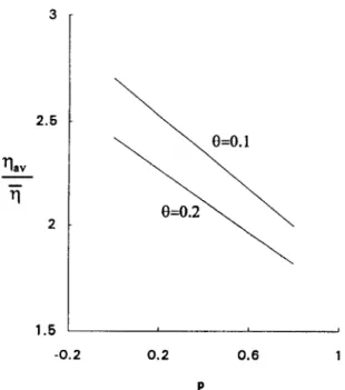
Defining q,“/?j as the learning gain enhancement relative to the l,-norm, Fig. 3 shows qBV/ij as

3 - 2.6 rl av T 2

o=o.

1 \ \ CM.2 1.6 ’ , -0.2 0.2 0.6 1 P

Fig. 3. Learning gain enhancement (q&) as a function of p under P(e) z 0.

a function of p under P(e) z 0. It can be seen that ~,~/ij increases with decreasing 0. However, small values of 8 may result in a numerical problem and hence 0 cannot be too small. Some empirical values of Q will be used in our later simulations.

In the decision-directed mode, 1 e(n)1 will be distributed in [e, 11. Therefore, qav can be obtained directly from (19) as

vl,y = (1 - e)(3 - p)(i - e3-p)-iq. If 83-p<< 1, (24) can be simplified as

(24)

vl ay z (1 - 0)(3 - PIN. (25)

4.2. I,-norm for 1 < p 6 2

Since no numerical problem occurs for

1 < p Q 2, qav can be obtained directly from (22) and (24) by setting t9 = 0. Therefore, in the training mode, ray becomes

qaV = (3 - p)[l + P(e)(23-P - 2)1-l& If P(e) c 0, (26) yields

(26)

&“%(3 -PI@ (27)

Finally, in the decision-directed mode, qaV is given by

9a” = (3 - PI6 (28)

The same results can also be found in c22]. Eq. (27) or (28) tells that qav can be, at most, enhanced by a factor of (3 - p). It is worth noting that the qav for the Ii-norm is twice of that for the 12-norm. This property is attractive since using Ir-norm can in- crease the convergence rate at a reduced computational complexity.

4.3. l,-norm in a higher signal-to-noise ratio environment

When the signal-to-noise ratio (SNR) is high, P(e) tends to be negligible and (e(n)1 can be bounded by a small value of c1< 1 in some cases. Accordingly, for p < 1, E[le(n)12-P] x E{le(n)12-Plle(n)lE[0,a]} with 8 <a 6 1, while for 1 <p < 2, E[le(n)12-P] z E{le(n)12-Plle(n)lE

(8)

152 C.-H. Chang et al. /Signal Processing 47 (1995) I45- 158

[0, LX]} with 0 < a < 1. Then we obtain

m4412-Pl

~

i

(a -

8))‘(3 - p)-‘(a+p - 83-p), p < 1, &P(3 - $1, lQp<2. (29) Therefore, in both training mode and decision-directed mode, vav becomes

x i (a - 8)(3 - p)(a3-p - 83-p)-1yl, p < 1, (3 - p)C2yi, l<p62. (30) 5. Computer simulations

A random sequence with alphabet { - 1, l} is used as the input to the channel for computer simulations. A zero-mean white Gaussian noise is used as the additive interference. A linear channel of the form

r(n) = 0.348s(n) + 0.870s(n - 1) + 0.348s(n - 2) (31) is first chosen to justify the effect of p on the performance results obtained above. The equalizer delay chosen is d = 2. Unless otherwise indicated, the order of polynomial expansion used is i = 3 for all the polynomial-perceptron based equalizers. The SNR is defined by SNR = 10 log(oz/oz), where a: is the signal power at the output of the channel and ai is the noise power. For the simplicity in representation, the notation (L, M) DFE is used to denote a DFE having L taps in the feedforward filter and M taps in the feedback filter. Also, the notation (N,, IV,, N3) MLP is used to denote an MLP having N1 neurons in the hidden layer 1, NZ neurons in the hidden layer 2, and N3 neurons in the output layer. The learning curves are determined by an average of 800 individual trials with each comprising different input sequences and different sets of random initial tap-weights. The BER performances are evaluated by an average of 800 independent trials with each comprising 10 000 bits in length. In each trial, the first 1800 bits are used for training,

which is considered sufficient for a nearly complete training. Furthermore, in the case of p < 1, some empirical values of 8 are used.

5.1. Convergence properties

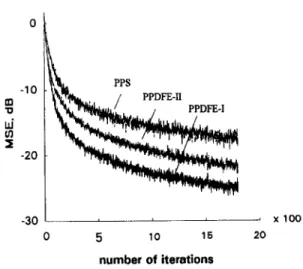
In these simulations, the MSE is used as a measure of the convergence performance and SNR = 20 dB is used in all simulations. Fig. 4 shows the learning curves of the (4,l) PPDFE-I, the (4, 1) PPDFE-II and a PPS equalizer of length 5. Here, the 12-norm algorithm with f = 0.1 and fi = 0.05 is used for all cases. The results indicate that the proposed structure (PPDFE-I) converges much faster than the PPDFE-II as well as the PPS equalizer. The former justifies the prediction in Section 2 and the latter demonstrates the benefit of using a DFE in such a single-layer net. Fig. 5 com- pares the learning curves between the (4,l) PPDFE-I and a (6,3, 1) MLP (4, 1) DFE. Here, a (6,3,1) MLP is chosen such that the number of tap-weights needed are comparable with the (4,l) PPDFE-I. The Z2-norm BP algorithm with f = 0.1 and /3 = 0.05 is used to train the MLP and the same parameters as above are again used in (4,l) PPDFE-I. It is seen that the (4, 1) PPDFE-I converges much faster than the MLP.

-10 B ! -20 -30 I x 100 0 5 10 16 20 number of iterations

Fig. 4. Comparison of convergence rate for different poly- nomial-perceptron based equalizers: PPS of length 5, (4,1) PPDFE-I and (4, 1) PPDFE-II.

(9)

Fig. 6 shows the effect of p on the convergence rate for the (4, 1) PPDFE-I. Here, different values of

p, 2, 1.2 and 0.6, are used to illustrate their effect on

the convergence rate. Other parameters used are: rj = 0.1 and 0 = 0.2 f or p = 0.6. The results indicate that significant improvement in convergence rate can be achieved by using smaller values of p. The dependence of convergence rate on p, with noise

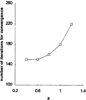
floor at - 20 dB, is shown in Fig. 7. It can be seen that the convergence rate increases with decreasing

p for p < 2. However, the convergence rate approaches a limit as further decreasing p from

’ xl00

0 6 10 16 20

number of iterations

Fig. 5. Comparison of convergence rate for the (4,l) PPDFE-I using i = 3 and the (6,3,1) MLP (4,1) DFE.

0 -10 i -20 J x -30 -40 -50 fig4.5,6-sigp677 ’ xl00 0 5 10 15 20 number of iterations

Fig. 6. Learning curves of the (4,1) PPDFE-I at different values Fig. 8. Convergence rate of the (4,1) PPDFE-I as a function

of p for SNR = 20 dB. 0f e.

certain values of p (say, p = 0.6). This is largely

caused by the constant 8 as well as the error probability P(e). Another reason might be resorted to the potential limit of the algorithm with stochastic gradient estimate. Fig. 8 shows the dependence of

260

0.2 0.6 1 1.4

P

Fig. 7. Convergence rate of the (4,l) PPDFE-I versus p.

1

0 0.2 0.4 0.6 0.8 1

(10)

154 C.-H. Chang et al. /Signal Processing 47 (1995) 145-158

convergence rate on 0 with noise floor at - 20 dB. As we have expected, the convergence rate decreases with increasing 0.

5.2. BER performances

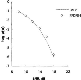
Unless otherwise indicated, detected-bit feedback is assumed in the following simulations of DFE. Fig. 9 gives a BER performance comparison for the (4, 1) PPDFE-I, the (4, 1) PPDFE-II, and the PPS equalizer of length 5. The result indicates that the proposed structure (PPDFE-I) outperforms the other two, especially in a higher SNR environment. Parameters used here are the same, except f = 0.03, as that used in Fig. 4. Fig. 10 com- pares the BER performance between the (4,l) PPDFE-I and the (6,3, 1) MLP (4,l) DFE. The simulation result indicates that the proposed structure is capable of achieving performance similar to that achieved by the MLP. Fig. 11 gives the BER performance of the (4,l) PPDFE-I as a function of p. The result indicates that the case using p = 0.6 outperforms those using larger values of p. The

0

1

+ PPS -1 -2 3 E-3 - 8 PPDFB-II, PPDFE-I

b

-6 I 6 10 14 18 22 SNR, dB

Fig. 9. BER performance for different polynomial-perceptron based equalizers: PPS of length 5, (4, 1) PPDFE-I and (4,l) PPDFE-II.

improvement becomes more significant when the SNR is high. This is because the equalizer achieves a better tracking capability, as described by (30), in

B-4 - -5 - -6 --- MLP 0 PPDFE-I -7 ’ 6 10 14 18 22 SNR. dB

Fig. 10. Comparison of BER performance for the (4, 1) PPDFE-I using i = 3 and the (6,3,1) MLP (4, 1) DFE.

0 - -1 - -2 - T z-3 . 8 -4 - -5 p=2 p=1.2 p=O.6 -6 ’ 6 10 14 18 22 SNR, dB

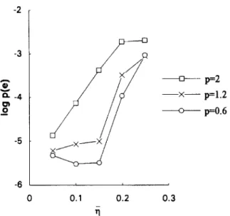
Fig. 11. BER performance for the (4,l) PPDFE-I at different values of p.

(11)

C.-H. Chang et al. /Signal Processing 47 (1995) 1455158 155 -3 3 x -4 8 -5 Table 1

Volterra coefficients for the nonlinear channel given by (32) and (33) - p=2 -x-- p=1.2 - p=O.6 Linear part c,, = 0.408 cr = 0.816 cz = 0.408 Second-order nonlinearities

co0 = 0.033 co1 = 0.067 err = 0.133 coz = 0.033 crz = 0.067 czz = 0.033 Third-order nonhnearities

coo0 = - 0.007 cool = - 0.041 co11 = - 0.082 c, 11 = - 0.054 coo2 = - 0.020 co12 = - 0.082 c1r2 = - 0.082 coz2 = - 0.020 Cl_?2 = - 0.041 c222 = - 0.007 -6 ’ 0 0.1 0.2 0.3 rl

Fig. 12. BER performance as a function of rj for the (4,1) PPDFE-I.

such a condition. It is worth noting that, besides a convergence rate improvement as indicated in Fig. 6, a BER improvement can also be achieved by using smaller values of p. This simulta- neous improvement cannot be achieved by an Z,-norm. Fig. 12 shows the BER performance of the (4, 1) PPDFE-I as a function of II. It can be seen that the performance using p = 2 is quite

sensitive to the noise caused by larger values of f [ll]. However, this is less serious when using p -c 2.

To see the ability of the new equalizer to cope with a nonlinear channel, a channel of the form

t(n) = 0.408s(n) + 0.816s(n - 1) + 0.408s(n - 2), (32)

r(n) = t(n) + 0.2?(n) - O.lt3(n) ₍₃₃₎

is chosen [3, 6, 181 for evaluating the performance of our approach. The linear part in (32) results in severe intersymbol interference, and the nonlinear part in (33) guarantees poor performance for the conventional DFE (CDFE). Combining (32) and

(33) yields the Volterra series representation [l] of the form

r(n) = i CiS(n - i) + i i CijS(n - i)S(n -j)

i=O i=O j=i

+ f: i i cijks(n - i)S(n - j)s(n - k), (34)

i=Oj=ik=j

with coefficients Ci, Cij and cijk given in Table 1. The

binary nature of s(n) makes it impossible to identify a nonlinear channel by using a direct modeling [6]. Consequently, an adaptive equalizer requiring a channel estimator, such as the adaptive MLSE, cannot perform well in such a situation.

Fig. 13 shows the BER simulation results of the (4, 1) Bayesian DFE [3-$91, the (4, 1) PPDFE-I,

Ol

+ Bayesian -X- PPDFE-I _ + CDFE -6- 4 8 12 16 20 24 SNR. dB

Fig. 13. Comparison of BER performance for the Bayesian (4,l) DFE, the (4, 1) CDFE, the (4,l) PPDFE-I and the MLSE under a nonlinear channel.

(12)

156 C.-H. Chang et al. JSignal Processing 47 (1995) 145&158

“I

z -2 z-3 _i

$

_-4_I -6

I

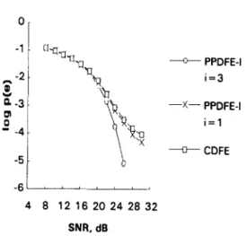
-6j 4 8 121620242832 SNR, d0 PPDFE-I i=3 -X- PPDFE-I i=l + CDFE

Fig. 14. Comparison of BER performance for the (2,3) PPDFE-I and the (2,3) CDFE under channel (35).

the (4,1) CDFE, and the MLSE under this nonlinear channel. Here, correct-bit feedback is assumed for all cases. Other parameters used are: I,-norm algorithm with p = 1.2 and f = /? = 0.1 for the PPDFE-I and LMS algorithm with # = 0.01 for the CDFE. Note that, in the LMS, q = 0.01 is deliberately chosen so that the CDFE can appro- ximately achieve its best possible performance. A correct estimate of the channel response is assumed for both the Bayesian criterion and the MLSE. The result demonstrates that our equalizer has a performance close to that offered by the Bayesian criterion, which is optimal in a minimum BER sense for symbol-by-symbol-decision equalizer. Also, it shows that the CDFE performs very poorly under the channel considered. This is due to its limited capabilities in partitioning the signal space.

Finally, to illustrate the advantage of higher- order expansion used in our structure, a linear channel with severe interference [lS] as described by

r(n) = 0.227s(n) + 0.460s(n - 1) + 0.688s(n - 2) + 0.460s(n - 3) + 0.227s(n - 4) ₍₃₅₎ is chosen to evaluate the performance. Fig. 14 com- pares the performance of a (2,3) PPDFE-I using

different orders of polynomial expansion (i = 1 and

i = 3) and a (2,3) CDFE. Note that correct-bit

feedback is again assumed for all cases. It is worth noting that the third-order PPDFE-I can equalize such a difficult channel, while the CDFE and the first-order PPDFE-I cannot perform well, under this condition. This justifies the benefit of using higher-order expansion over the signal vector presented in a DFE.

6. Comparison with other nonlinear equalizers It is known that the performance of the equalizer with detection based on the entire sequence can be better than those based on a symbol-by-symbol basis, provided that the characteristic of the channel is known. However, if the channel response is not known a priori, a procedure of channel estimation is necessary [ 1.51. An inaccurate estimate may degrade the performance. The new equalizer does not require a channel estimate yet achieves a performance comparable to the Bayesian criterion. Furthermore, the implementation complexity of the MLSE may preclude its use in some real-time applications. Although the use of Viterbi algorithm [7] may reduce the complexity significantly, the requirement of computations and memory is still demanding. The new approach has much less de-

manding in computation and no memory

requirement.

In [6], Chen et al. showed that the radial basis function (RBF) equalizer and the optimal Bayesian solution are equivalent in structure. The result indicated that the RBF equalizer has similar performance to the Bayesian approach given a known channel order and noise variance. However, performance degradation occurs when the above parameters are not known a priori. Our approach achieves similar performance without any knowledge of the channel and the noise.

One disadvantage of our structure is its large number of tap-weights needed in some practical applications. Fortunately, a number of higher- order terms that tend to be inconsequential can be neglected. A good example for this can be found in [l]. It indicated that a significant MSE

(13)

improvement can be achieved even using only a few nonlinear terms for the equalization over a nonlinear satellite channel.

7. Conclusions

A new equalizer, including a DFE equipped with polynomial-perceptron model of nonlinearities and an [,-norm based robust learning algorithm, is presented in this paper. The structure exerts the benefit of using a DFE with a polynomial-perceptron structure. The algorithm is robust in the sense of dealing with aberrant noise by the effect of p < 2 on the error signal. A detailed performance analysis of the algorithm including a consideration on the possible numerical problem arising when p < 1 is given in this paper. The algorithm is advantageous due to its robustness as well as its simplicity. Computer simulation results show that the proposed equalizer simultaneously accomplishes faster convergence rate and satisfactory BER performance. Parti- cularly, it is shown that our equalizer can approach the performance offered by the Bayesian criterion and achieves significant improvement in BER performance for channels having severe interference.

Acknowledgements

The authors would like to thank the anonymous referees for their valuable comments to improve the manuscript.

Notation

P threshold level adaptation gain

d equalizer delay

VLJ gradient vector in the p-power error surface

% gradient vector estimate in the p-power error surface

8 change of error at p = 2

e error signal

E expectation operator

&P l,-norm error function

'P

12

M

p(e)

P r S

w

2 0” 2 0s 8 u UO V W

w

0 X xF Xtl Y Z learning gain learning gain at p = 2 average learning gain

effective learning gain at arbitrary values of P

learning gain enhancement activation function first derivative off

order of polynomial expansion

number of taps in the feedforward part of a DFE

p-power error metric mean squared error metric

number of taps in the feedback filter of a DFE

time index

number of weights needed for the perceptron

error probability in making decisions power of error metric

output of a channel transmitted signal sign operator noise power signal power

small positive number perceptron input vector input of unity value decision error

perceptron weight vector threshold level for the perceptron input vector represented by a DFE feedforward signal vector in X feedback signal vector in X perceptron output

error suppressor function

References

Cl1 M

IL31

S. Benedetto, E. Biglieri and V. Castellani, Digital Trans- mission Theory, Prentice-Hall, Englewood Cliffs, NJ, 1987. C.H. Chang, S. Siu and C.H. Wei, “A decision feedback equalizer utilizing higher-order correlation”, Proc. 1993

IEEE ISCAS, Chicago, IL, May 1993, pp. 707-710. S. Chen, G.J. Gibson, C.F.N. Cowan and P.M. Grant, “Adaptive equalization of finite non-linear channels using multilayer perccptrons”, Signal Processing, Vol. 20, No. 2, June 1990, pp. 107-119.

(14)

158 C.-H. Chang et al. jSigna1 Processing 47 (1995) 145~158

[4] S. Chen, G.J. Gibson and C.F.N. Cowan, “Adaptive chan- [ 151 F.R. Magee and J.G. Proakis, “Adaptive maximum-likeli- nel equalization using a polynomial-perceptron structure”, hood sequence estimation for digital signaling in the pres-

IEE Proc., Pt. I, Vol. 137, No. 5, 1990, pp. 257-264. ence of intersymbol interference”, IEEE Trans. Inform.

[S] S. Chen, G.J. Gibson, C.F.N. Cowan and P.M. Grant, Theory, Vol. IT-19, 1973, pp. 12&124.

“Reconstruction of binary signals using an adaptive radial- [16] M. Minsky and S. Papert, Perceptron: An Introduction to

basis-function equalizer”, Signal Processing, Vol. 22, No. 1, Computational Geometry, MIT Press, Cambridge, MA,

January 1991, pp. 77-93. 1988.

[6] S. Chen, B. Mulgrew and P.M. Grant, “A clustering technique for digital communications channel equalization using radial basis function networks”, IEEE Trans. Neural Networks, Vol. 4, No. 4, 1993, pp. 570-579.

[7] G.D. Forney, “Maximum-likelihood sequence estimation of digital sequences in the presence of intersymbol interference”, IEEE Trans. Inform. Theory, Vol. IT-18 1972, pp. 363-378.

[17] Y.H. Pao, Adaptive Pattern Recognition and Neural Net- works, Addison-Wesley, Reading, MA, 1989.

[18] J.G. Proakis, Digital Communications, McGraw-Hill, New York, 1989.

[19] A.K. Rigler, J.M. Irvine and T.P. Vogl, “Resealing of variables in back propagation learning”, Neural Networks,

Vol. 4, 1991, pp. 2255229. [S] W.S. Gan, J.J. Soraghan and T.S. Durrani, “New func-

tional-link based equalizer”, Electron. Lett., Vol. 28, No. 17, August 1992, pp. 1643-1645.

[9] G.J. Gibson, S. Siu and C.F.N. Cowan, “The application of nonlinear structures to the reconstruction of binary signals”, IEEE Trans. Signal Process., Vol. 39, No. 8, 1991, pp. 1877-1884.

[20] D.E. Rumelhart and J.L. McClelland, Parallel Distrib- uted Processing: Explorations in the Microstructure of Cognition, MIT Press, Cambridge, MA, 1986, Vol. 1, Chapter 8.

[lo] F.R. Hampel, E.M. Ronchetti, P.J. Rousseeuw and W.A. Stahel, Robust Statistics: The Approach based on Injuence Functions, Wiley, New York, 1986.

[ 1 l] S. Haykin, Adaptive jilter theory, Prentice-Hall, Engle- wood Cliffs, NJ, 1991.

[12] P.J. Huber, Robust Statistics, Wiley, New York, 1981. [13] B. Kosko, Neural Networks and Fuzzy Systems: A Dynam-

ical Systems Approach to Machine Intelligence, Prentice- Hall, Englewood Cliffs, NJ, 1992.

[14] R.P. Lippmann, “An introduction to computing with neural nets”, IEEE ASSP Magazine, April 1987, pp. 4-22.

[21] J. Schroeder, R. Yarlagadda and J. Hersey, “ldp normed minimization with applications to linear predictive modeling for sinusoidal frequency estimation”, Signal Pro- cessing, Vol. 24, No. 2, August 1991, pp. 1933216. [22] S. Siu and C.F.N. Cowan, “Performance analysis of the

Ir,-norm back propagation algorithm for adaptive equalization”, IEEE Proc., Pt. F, Vol. 140, No. 1, 1993, pp. 43-47.

[23] S. Siu, G.J. Gibson and C.F.N. Cowan, “Decision feedback equalization using neural network structures and performance comparison with standard architecture”, IEE Proc.,

Pt. I, Vol. 137, No. 4, August 1990, pp. 221-225. [24] B. Widrow, R.G. Winter and R.A. Baxter, “Layered neural

nets for pattern recognition”, IEEE Trans. Acoust. Speech Signal Process., July 1988, pp. 10961099.

A polynomial-perceptron based decision feedback equalizer with a robust learning algorithm