半導體產業大型廠房之設施規劃

(1)

行政院國家科學委員會補助專題研究計畫

□

成果報告

■

期中進度報告

半導體產業大型廠房之設施規劃

畫類別：個別型計畫計畫編號：NSC 96－2628－E－009－026－MY3 執行期間： 2007 年 8 月 1 日至 2010 年 7 月 31 日計畫主持人：巫木誠共同主持人：計畫參與人員：施昌甫、陳振富成果報告類型(依經費核定清單規定繳交)：■ 精簡報告 □完整報告本成果報告包括以下應繳交之附件： □ 赴國外出差或研習心得報告一份 □ 赴大陸地區出差或研習心得報告一份 □ 出席國際學術會議心得報告及發表之論文各一份 □ 國際合作研究計畫國外研究報告書一份處理方式：得立即公開查詢執行單位：國立交通大學工業工程與管理學系中華民國 97 年 5 月 29 日

(2)

半導體產業大型廠房之設施規劃國科會計畫編號：NSC 96－2628－E－009－026－MY3 主持人：巫木誠交大工業工程與管理系

摘要

電子產品的需求大增，造成半導體晶圓的需求也逐年增加，許多公司都不斷的興建新的晶圓廠，形成公司擁有許多相鄰近晶圓廠的趨勢。而雙廠區的建置更逐漸形成半導體產業未來的趨勢，如何將產品所需要的產能配置給相鄰近的晶圓廠形成一重要的問題。過去有許多的相關文獻探討此問題，但其大部分假設廠區間產能無法跨廠支援。本研究欲發展一演算法在產能可跨廠支援的情境下規劃產品的途程與產能配置，使平均的生產週期時間最短。先利用線性規劃取得初始的途程規劃解，再利用基因演算法與等候理論的評估工具來獲得最佳的途程規劃解。然後利用模擬來驗證此途程規劃解的正確性。最後本研究並分析比較產能可互相支援與不能互相支援的績效差異。關鍵字：雙廠區、跨廠途程、途程規劃、產能支援

Abstract

This paper formulates and solves a route planning problem for semiconductor manufacturing. In order to quickly respond to demand booming, a semiconductor company usually adopts a

dual-fab strategy in expanding capacity. That is, two fab sites are so built that they are

neighbor to each other, and can easily share capacity. Through the capacity–sharing design, a product may be produced by a cross-fab route. That is, some operations of a product are manufactured in one fab and the other operations in the other fab. This leads to a routing planning problem, which involves two decisions—determining the cutoff point of the cross-fab route and the route ratio for each product—in order to maximize the throughput subject a cycle time constraint. An LP-GA method is proposed to solve the route planning problem. We first use the LP module to make the cutoff point decisions, and proceed to use the GA module for making the decision of route ratio. Experiment results show that LP-GA method significantly

(3)

outperforms the other methods.

Keywords: dual-fab, cross-fab route, route planning, capacity sharing.

1. Introduction

Semiconductor manufacturing industry has three characteristics in expanding capacity. The cost of equipment is very expensive, maybe costing over one billion dollars for a 12 inch wafer fab. The lead time for equipment acquisition is quite long, ranging from 3 to 9 months. Yet, building the factory space is relatively low in expense but with a much longer lead time—taking about one to two years.

In order to quickly respond to demand booming, a semiconductor company usually adopts a dual-fab strategy in expanding capacity. That is, a large-scale factory space that could accommodate two fabs is established in advance. Then, equipments for the two fabs are gradually moved into the space according to the market demand over time. The two fabs, so close to each other in location, are eligible to support capacity to each other, and should be managed in an integrated manner. .

In such a dual-fab configuration, a relatively easy way to manage is manufacturing each wafer job in one fab. That is, each fab is run separately, without any mutual support in capacity. Such a separated-operation paradigm would usually lead to the underutilization of equipment. To remedy the underutilization issue, a cross-fab production paradigm is proposed. This means that a wafer job is partly manufactured in one fab and partly manufactured in the other fab.

Such a cross-fab production paradigm yields a route planning problem—how to appropriately assign the operations of a wafer job to each of the two fabs. Only a few studies on the route planning problem have been published. Toba et al. (2005) addressed the route planning problem in a real-time manner. That is, whenever an operation of a job is completed, a decision—which fab to manufacture the next operation—must be immediately made. Wu and Chang (2006) investigated the route planning problem in a short-term or weekly manner, in which the two fabs exchange capacity weekly to maximize the total throughput.

Though having established significant milestones, these two prior studies have some limitations due to make an implicit assumption. They both assumed that the transportation

(4)

times within a fab or among fabs are a constant. This implies that the transportation capacity is infinite, and the route planning algorithm may yield a solution with too much transportation. This may lead to traffic jam and as a result may lower the throughput and lengthen the cycle time.

In semiconductor manufacturing, the wafer size has steadily increased over time. In an up-to-date fab (12 inch wafer fab), wafer jobs must be transported by automatic vehicles because a wafer job weighs about 30 kg and cannot be handled manually. This may yield a traffic jam problem because the transportation capacity is limited. Our interview with practitioners indicates that the traffic jam symptom would occur, in particular for a dual-fab layout. Therefore, transportation capacity has to be considered in the route planning problem for an up-to-date fab.

This research investigates the route planning problem for a dual-fab layout and is unique in two-fold. First, we assume that the transportation capacity is finite and the transportation times would vary. Second, the route planning decision is made based on a relatively longer time horizon—for example, one or several months. This research, focusing on a relatively long-term decision, complements prior studies which focused on either short-term or mid-term decisions on route planning.

The remainder of this paper is organized as follows. Section 2 reviews literature relevant to this research. Section 3 presents the route planning problem in detail. Section 4 described the solution framework that includes a linear programming (LP) model, a binary search algorithm, a queuing net work model, and a genetic algorithm (GA). Section 5 describes the LP model and the binary search algorithm. Section 6 describes the queueing model and the GA. Numerical experiments are presented in Section 7 and concluding remarks are in the last section.

2. Relevant Literature

Given a customer demand, there may exist more than one manufacturing sites to fulfill the demand. A decision problem is how to allocate the demand to each manufacturing site. This capacity allocation problem can be addressed either in product level or in operation level.

For the problem in the product level, each site is designated to manufacture a set of products. This implies that a product should be completely manufactured within a single

(5)

site—cross-site production is prohibited. While in the operation level, each site is designated to manufacture a group of operations. Then, the operations for manufacturing a product could be distributed among different sites—cross-site production is allowed. This leads to the need for studying the route-planning problem.

For the capacity allocation problem—without any cross-site routes, Wu et al. (2005) have given a comprehensive survey. Some recent studies are listed (Rupp ＆ Ristic 2000; Frederix 2001; Karabuk ＆ Wu 2003; Manmohan 2005; Lee et al. 2006; Chiang et al. 2007). Linear programming models are commonly used to solve the problems. To address the interactions among manufacturing sites, game theory was proposed to enhance the LP model (Mieghem 1999).

For the capacity allocation problem—with some cross-site routes, most studies were addressed in the context of group technology (GT). That is, each site is a manufacturing cell and multiple cells form a factory. Cross-cell production for manufacturing a product is permitted. However, each product is preferably manufactured within a particular cell and cross-cell production should be minimized.

Most prior studies allocated the capacity demand to cells through solving a cell formation problem (Avonts ＆ Wassenhove 1988; Kim et al. 2005; Vin et al. 2005; Dimopoulos 2006; Mahdavi 2006; Nsakanda et al. 2006; Spiliopoulos ＆ Sofianopoulou 2007). That is, in order to minimize the number of cross-cell transportations, researchers have to answer how many cells should be formed and how each cell should be equipped. After the cell formation problem is solved, each product is assigned to a particular cell for handling most of its operations. The remaining operations, much fewer in number, are handled by other cells. A GT cell is designed for manufacturing a particular group of products, and by nature is limited in its functional capacity. Therefore, cross-cell routes are unavoidably demanded in GT in order to enhance its functional spectrum.

However, in the route-planning problem we address, each of the two fabs is assumed to be functionally comprehensive. That is, a product can be completely manufactured in either one of the two fabs. The purpose of cross-fab production is to increase the total throughput of the two fabs, with the rationale explained below.

(6)

which is generally obtained from the demand forecast at the time of purchasing equipment. However, the market demand in terms of product mix may change over time. Therefore, a fab may be underutilized due to a change of product mix. In addition, the two fabs, even both functionally comprehensive, may differ in number for each type of machines. This implies that their originally designed product mixes may also differ. Cross-fab production therefore is needed to increase the total throughput of the two fabs.

3. Problem Statement

This section aims to describe the dual-fab route planning problem more precisely. We first present the assumptions that confine the context of the route planning problem; and then proceed to introduce the decision variables, objective function and constraints of the problem. In explaining the assumptions, the two fabs are respectively called Fab_A and Fab_B.

Assumption 1: Each fab is functional comprehensive. Each of the two fabs is so

comprehensively equipped that it can handle the manufacture of each product by itself—not requiring the functional support of the other fab.

Assumption 2: A product has four possible routes. To implement cross-fab production, the

manufacturing route of a product is cut into two parts, where the route‘s break point is called a

cut-off point. The two parts can be manufactured in different fabs, and yield two possible

routes for cross-fab production. One, represented by , denotes that the first part of the route is manufactured at Fab_A and the second part is at Fab_B. The other one, represented by



  , denotes that the first part of the route is at Fab_B and the second part is at Fab_A. Since each fab is functionally comprehensive, a product thus has four possible manufacturing routes,  ,  ,  , and  , where  denotes a route at Fab_A only and  denotes a route at Fab_B only.

Assumption 3: The transportation path between any two workstations/buffers is unique, rather than multiple. In each fab, a transportation system for moving wafer jobs has been

established. Theoretically, there may exist multiple paths in transporting a wafer job from a workstation to another; however, to reduce the complexity of traffic control, we predefine a fixed path for such a transport.

The route planning problem has two decision variables for each product: its cutoff point and the ratios of its four possible routes (simply called route ratios). Let the cutoff point and

(7)

route ratios of product i be represented by ( , )_i r_i . Herein, i denotes the identification code

(an integer) of the operation for separating a route into two parts; and r_i [ , , ,a b c d_i _i _i _i] is a four-element vector where each element denotes the percentage of a particular route—of the four ones  ,  , , and  . Define  [ ,...,1 n] as a set of cutoff points and

] ,..., [r₁ r_n

R = as a set of route ratios for n products to be produced. The route planning problem is to determine a (*,R*) in order to maximize the total throughput of the two fabs, subject to the constraint of meeting a target cycle time.

4. Solution Framework

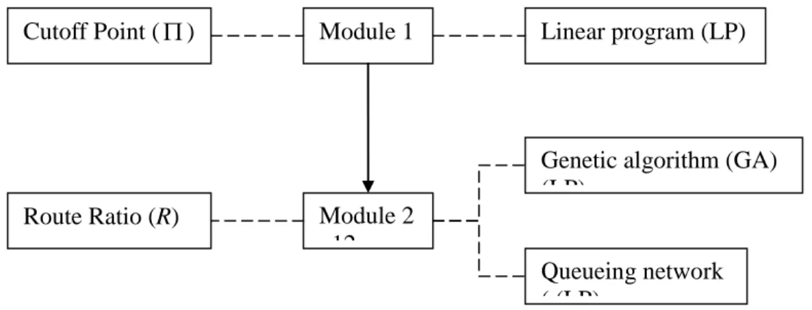
A framework proposed for solving the dual-fab route planning problem is shown in Fig. 1, which involves two modules.

<<Insert Fig. 1 about here>>

In Module 1, each transportation path is assumed to be equipped with infinite capacity; and the transportation time between any two workstations/buffers is zero. With the routing problem so simplified, we attempt to find an optimum, in terms of minimizing the total number of inter-fab transportations. The problem is solved by an iterative use of a linear program (LP) model. For a particular, the LP model aims to compute its minimum number of inter-fab transportations, which is regarded as the performance of the. We then use a binary search algorithm to identify an optimum *as the ultimate decision for cutoff point.

In Module 2—with the obtained *taken as parameters, we deal only with the decision variables R =[r₁,...,r_n]. In this module, each transportation path is taken as a tool with limited capacity. The transportation time required for passing through a path can be varied, depending upon the traffic flow intensity. The higher the traffic intensity, the longer is the cycle time.

Module 2 involves two sub-modules. The first one aims to develop a performance evaluator for a particular ( , ) R . To do so, we first construct a queueing network model (Connors et al.1996) in order to compute the resulting mean cycle time, subject to a target throughput and a particular ( , ) R . The queueing model is further enhanced as follows. Subject to a target mean cycle time and a particular( , ) R , the enhanced model could compute the resulting throughput—the performance of the ( , ) R .

(8)

search an R so that the performance * (*,R*) is the best. A genetic algorithm is proposed to solve the search problem—finding the ultimate decision of R.

In summary, the solution space of the dual-fab routing planning problem can be described by S ={( , ) | R _Set R, R Set_ }. The objective is to find an optimum

* *

( ,R ) from S, in terms of maximizing throughput subject to a target cycle time. Since the number of elements in S can be very huge, the problem is decomposed into two sub-problems. The first one is to find an optimum*, and the second sub-problem proceeds to find an optimum R by taking * *as predefined parameters.

The essences of these two modules are compared below. Module 1 essentially deals with a

static capacity allocation problem which does not consider job flow time. In contrast, Module

2 deals with a time-phased capacity allocation problem, in which job flow time is addressed and computed by a queueing network model.

Without addressing job flow time, Module 1 needs not considering the transportation times of jobs. This leads to the underlying assumption of Module 1—the transportation time between any two workstations/buffers is zero. While the underlying assumption is released, we have to consider job flow time in Module 1. Solving such a problem is very computational extensive because it may need an iterative evaluation of a linear program embodied with a discrete event simulation program, as proposed by Hung and Leachman (1996).

5. Module 1－LP Model and Search Algorithm

Obtaining the solution for Module 1 is through an iterative use of an LP program. We first describe the LP model and then present the iterative method—a bi-section search algorithm.

Indices

i: index of product

g : index of workstation in Fab_A h: index of workstation in Fab_B

Parameters

(9)

i

 : cutoff point for defining the cross-fab routes of product i

:  [ ], 1_i  i n, a vector for describing the cut-off points of all products

Q: an estimated total throughput of the two fabs while in high utilization (in lots), which is used as the target throughput in the LP model.

i

P: percentage of product i in the product mix,

1 =1, 0 1 n i i i P P   



g

C : available machine hours of workstation g in Fab_A

h

C : available machine hours of workstation h in Fab_B

a

m : total number of workstations in Fab_A

b

m : total number of workstations in Fab_B

a ig

W : total processing time per lot required on workstation g in Fab_A, while product i is

manufactured by route 

c ig

W total processing time per lot required on workstation g in Fab_A, while product i is

manufactured by route 

d ig

W : total processing time per lot required on workstation g in Fab_A, while product i is

manufactured by route  

b ih

W : total processing time per lot required on workstation h in Fab_B, while product i is manufactured by route 

c ih

W : total processing time per lot required on workstation h in Fab_B, while product i is manufactured by route 

d ih

W total processing time per lot required on workstation h in Fab_B, while product i is manufactured by route  

Decision Variables

i

a : percentage of using route  in producing product i

i

b : percentage of using route  in producing product i

i

(10)

i

d percentage of using route   in producing product i

5.1 LP Model

The LP program is to compute a minimum number of cross-fab transportation for a particular --a decision for the route cutoff points, which has been known before solving the LP problem. The objective function of the LP program is denoted by Z().

Min 1 ( ) ( ) n i i i i Z Q P c d   



   s. t. ai  bi ci di 1 1 i n (1) 1 ( ) n a d c i i ig i ig i ig g i Q P a W d W c W C         



1 g m_a (2) 1 ( ) n b d c i i ih i ih i ih h i Q P b W d W c W C         



1 h m_b (3)

The objective function is to minimize the number of cross-fab production lots. The rationale for defining this objective is that cross-fab production requires longer transportation time than within-fab production. Subject to a target cycle time, an attempt to minimize cross-fab production lots tends to increase total throughput. Constraint (1) describes the dependent relationship among the route ratios. Constraints (2) and (3) ensure that the capacity used in each workstation, for Fab_A and Fab_B, should be lower than its available supply.

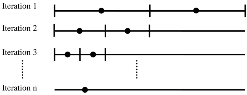
5.2 Bi-section Search Algorithm

The bi-section search algorithm is to find an optimum solution * from a space, denoted by {}, which is the possible combinations of cutoff points for all products. The algorithm is an iterative process. In an iteration, each product has only two possible cutoff points to select. Taking a product route as a line, the two cutoff points are respectively on the first and the third quartiles (Fig 2). By evenly cutting the route into two segments, each cutoff point is in the middle of a particular segment. Of the two evenly divided segments, the one where a cutoff point stays is called the housing-segment of the point.

(11)

In each iteration i, the size of the space {} is 2n if there are n products. By solving the LP program in an exhaustive manner (i.e., 2n

times), we can obtain the best solution in this iteration--denoted by *

i

 , which defines an optimum set of cutoff points. For each product, the

housing-segment of the cutoff point obtained is called the-segment (i.e., remaining segment) of the product, which is the output of iteration i and will be the input of iteration i+1. The bi-section search algorithm is summarized below.

Algorithm Search _Cutoff_Points Initialization

 For each product, take the whole route as its-segment. For i = 1 to N

 Create the two cutoff points on the-segment for each product  Solve LP programs in an exhaustive manner to find *

i

  Compute the-segment for each product based on *_i End for

Output the cutoff points for each product

6. Module 2—Queueing and GA

The problem to be solved in Module 2 can be stated as follows. Given a target cycle time (CT₀) and a cutoff point decision (*

) obtained from Module 1, we attempt to find an optimal route ratio decision R =[r₁,...,r_n] in order to maximize the total throughput of the two fabs subject that the corresponding average cycle time is less than CT₀.

This problem is essentially a space search problem, with a solution space

1

{ } {[ ,... ]|n _i ( , , ,_i _i _i _i)}

H R  r r r  a b c d . A genetic algorithm is proposed to solve the problem. In the algorithm, the fitness (performance) of a solution R is evaluated by a queueing network model. We first introduce the queueing network model and proceed to the genetic algorithm.

6.1 Queueing Network

(12)

(1996). The I/O function of the model developed by Connors et al. (1996) can be briefly formulated as follow: CT f TH R( , ,). That is, given a target total throughput (TH), a route ratio decision (R), and a cutoff point decision (), the queueing model (f) can be used to compute the two fabs‘ mean cycle time (CT). However, Connors et al. (1996) did not consider the effect of transportation among workstations.

We extended the application of their model based on two assumptions. First, we assume that the transportation path between any two stations is unique, where a station is either a workstation or a WIP storage buffer. Secondly, each transportation path between any two stations is modeled as a ―conveyor machine‖ with only one unit of capacity. Such an extension makes the developed queueing model closer to a semiconductor fab in the real world. Likewise, the I/O function of the extended queuing model can also be described as CT f TH R( , ,).

The objective function in Module 2 is to maximize throughput (TH) subject to a target cycle time (CT0). To evaluate the objective function, we used a bi-section search technique to

find the total throughput (TH) for a particular route ratio (R); that is TH  f R( ,*,CT0)

where *denotes the cutoff point decision obtained in Module 1 and CT0 is the target cycle

time. Notice that, for the function CT f TH R( , ,*), the higher the TH value, the higher is the CT value. The bi-section search technique, based on CT f TH R( , ,*), is intended to search a value for TH so that CT CT₀. The bi-section search algorithm is just like that of the binary search for a particular point on a line segment.

6.2 Genetic Algorithm

The genetic algorithm (GA) is to identify an optimal solution R from the space {R}. As *

stated, the performance of R is obtainable by the enhanced queueing model. A possible solution

R (or called a chromosome) is represented by a vector R[ ,... ]r₁ rn where r_i ( , , ,a b c d_i _i _i _i).

We call r a gene-segment and each of its element a gene, and the gene values are imposed _i

by the following constraints: a_i  b_i c_i d_i 1 and 0a b c d_i, , ,_i _i _i 1.

The GA is an iterative algorithm which can be briefly described as follows. Procedure GA

(13)

 t = 0, Status = ‗Not-terminate‘

 Randomly generate Npvalid chromosomes to form a population P0

Step 2: Genetic Search

While (Status = ‗Not-Terminate‘) do

 Use cross-over operator to create Nc new chromosomes

 Use mutation operator to create N_m new chromosomes

 Form a pool by taking the union of Pt and the set of newly created

chromosomes

 t = t + 1, and select the best Npchromosomes from the pool to form Pt

 Check if termination condition is met; if yes, set Status = ―Terminate‖ Endwhile

Step 3: Output the best chromosome R in Pt*

The crossover operation is to create two new chromosomes (say, R3 and R4) from two existing ones (say, R1 and R2). Let each gene-segment i in R1 and R2 be respectively represented by r and _i₁ r . We proposed a one-point crossover operation (Binh & Lan 2007) _i₂

on gene-segments r and _i₁ r to create two new ones _i₂ r and _i₃ r , which in turn could yield _i₄

two new chromosomes: R₃[ ]r_i₃ , R₄[ ], 1r_i₄  i n.

The one-point crossover operation on a gene-segment is briefly introduced. For two gene-segments (i.e., r and _i₁ r ), we randomly choose a gene, swap their gene values, and _i₂

modify another gene values in order to ensure a constraint satisfaction . Consider an example where the 2nd gene is chosen as the cross-over point for mixing r_i₁(a b c d_i₁, _i₁, _i₁, _i₁) and

2 ( 2, 2, 2, 2)

i i i i i

r  a b c d . By the swap and modification operations, we would obtain

3 ( 1, 2, 1,1 1 2 1)

i i i i i i i

r  a b c a b c and r =_i₄ (a_i₂,b_i₁,c_i₂,1-a_i₂-b_i₁-c_i₂).

In the mutation operation, a new chromosome (say, R2).is created by an existing one (say, R1). The mutation algorithm creates R2 by modifying a particular gene-segment in R1. The

modified gene-segment is randomly chosen. While being selected, two of its genes are randomly chosen and their gene values are swapped. For example, if gene-segment i*

(14)

is chosen for modification; and the 2nd and 4th genes are chosen to swap for

*₁ ( _i₁, _i₁, _i₁, _i₁)

i

r  a b c d , then r_i*₂ (a d c b_i₁, _i₁, _i₁, _i₁), which in turn yield a new chromosome

* 1 2 [ ,..11 i 2,... n] R  r r r from ₁ ₁₁ * 1 1 [ ,.. ,... n ] i R  r r r .

Two termination conditions are defined for the GA. First, the best solution in Pt has been

no change for over a certain period (say, Tb iterations). Second, population Pt has evolved over

a certain number of iterations; that is, t has reached its predefined upper bound (Tu).

7. Experiments

7.1. Benchmarks and Data

By using numeric experiments, we attempt to evaluate the effectiveness of the proposed method. Two other methods are used as benchmarks for comparison. The proposed method is designed as LP-GA, where LP denotes the linear program, GA denotes the genetic algorithm. The two benchmark methods are special cases of LP-GA. The first one is called M-GA, which denotes that the cutoff point of each route has been predetermined—just on the middle of the route. The second one is called N-GA, where denotes that cross-fab production is not allowed. Such a comparison is to tell how much benefit a dual-fab would obtain if the LP-GA method is used.

In the dual-fab experiments, the data for machines and product routes are adapted from an HP-fab in literature (Wein 1988). Of the two fabs, one involves 93 machines and the other involves 72 machines. Being functionally identical, each fab involves 4 batch workstations and 21 series workstations. The MTBF (mean time between failure) and MTTR (mean time to repair) of each machine is available, exponentially distributed. Three types of products are produced. One product involves 150 operations; the other two both involve 172 operations but are different in processing times. In implementing the GA, we set Tb = 1000, Tu = 30, P0 = 100, Pcr = 0.8, and Pm = 0.1.

7.2 Performance Comparison

The three methods are compared in two scenarios, with product mixes RA = (3:2:5) and RB

= (5:4:1) respectively. For each product mix, by the queueing model, we obtain a throughput level that will keep the two fabs in high utilization: QA = 128 lots and QB = 169 lots.

(15)

We compare the three methods from two perspectives. First, given a target throughput level, the mean cycle time of each method is compared. In the comparison, QA and QB are used as the target throughput levels. Second, given a target cycle time, we compare the throughput of each method. In the comparison, we set CT0 =11,081 min. for RA and CT0 =11,445 for RB.

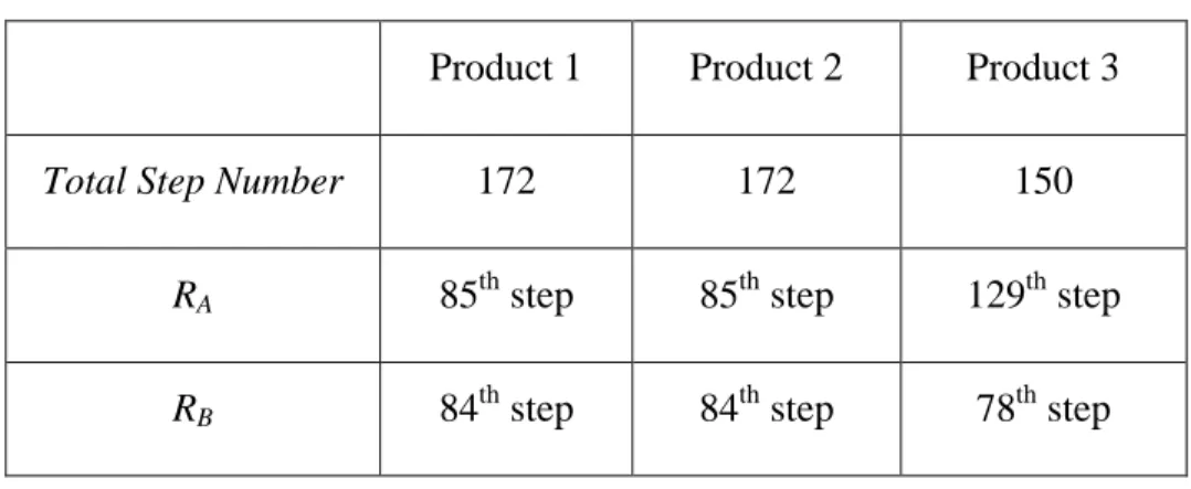
The cutoff points of each route obtained by the LP-GA method are shown in Table 1, which indicates that the cutoff points suggested by the LP-GA are different from that of M-GA.

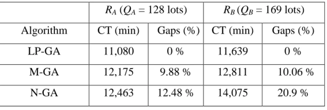
Table 2 shows the comparison of mean cycle times, subject to a target throughput. The

LP-GA outperforms the two benchmark methods. Using the result of LP-GA as a baseline, the

cycle time of the LP-GA method is about 10 % better than that of M-GA, and about 12-20% better than that of N-GA. This implies that managing a dual fab by adopting an optimum cross-fab production policy tends to shorten the cycle time—significantly better than managing each fab independently (i.e., no cross-fab production).

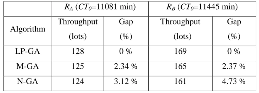
Table 3 shows the comparison of throughput, subject to a target cycle time. The LP-GA method also outperforms the two benchmark methods. Using the result of the LP-GA as a baseline, the throughput of the LP-GA method is about 2.3% higher than that of M-GA, and about 3.1-4.7% higher than that of N-GA. This implies that optimal planning of cross-fab production is positive in increasing throughput.

<<Insert Table 1 about here>> <<Insert Table 2 about here>> <<Insert Table 3 about here>>

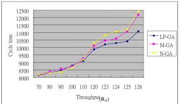
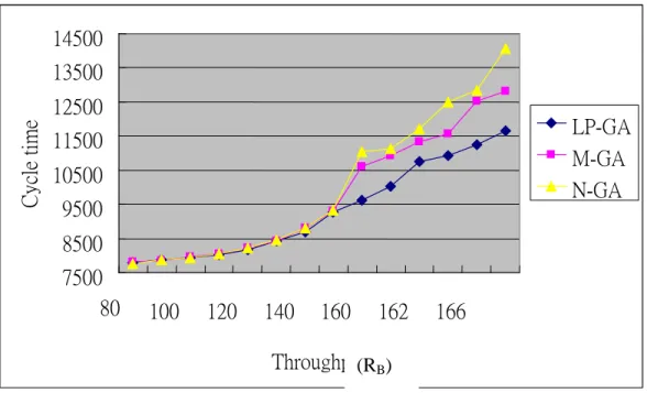
Figs. 3 and 4 reveal the relationship between cycle time and throughput for product mixes

RA and RB respectively. The higher the throughput, the longer is the cycle time. The two figures

also show that the higher the throughput, the larger is the performance gap. That is, the contribution of the LP-GA method becomes higher while it is applied in a high market-demand scenario.

<<Insert Fig. 3 about here>> <<Insert Fig. 4 about here>>

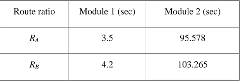
7.3 Complexity Analysis

(16)

4. The table indicates that the computation effort of Module 2 is much greater than that of Module 1. Each of the two modules essentially deals with a space-search problem—attempting to find an optimal solution from a solution space. Module 1 adopts an analytic approach (a linear program) while .Module 2 adopts a meta-heuristic approach (GA). A complexity analysis for Module 1 is therefore analyzed below.

<<Insert Table 4 about here>>

In Module 1, the iterative use of linear program is based on a binary-search method. For a scenario with n product and each product involves 1

2x  m 2x operations, the number of linear programs we have to perform is N  x 2n. For a scenario with n = 3 and m = 172, we need to perform the linear program about 8 2 364 times, which computationally takes only about 4 sec. The computation time will significantly increase if n is greatly increased.

To deal with the scenarios with large n, a future work of this paper can be investigated. We need to develop a product clustering module. Out of the n products, only a limited number (say, c) are considered for cross-fab production; the remaining n-c products are only be eligible for single-fab production.

8. Conclusion

This paper presents an approach to solve the route planning problem for a semiconductor dual-fab. In the problem, each product can be manufactured in either fab. And each product has four possible production routes, which are defined by a cutoff point. The route planning problem involves two decisions—determining the cutoff point and the route ratio for each product—in order to maximize the throughput subject a cycle time constraint.

An LP-GA method is proposed to solve the route planning problem. We first use the LP module to make the cutoff point decisions, and proceed to use the GA module for making the decision of route ratio. The LP-GA method is compared with two benchmark methods by numerical experiments. Results show that the LP-GA method significantly outperforms the other methods.

Some extensions of this research are being considered. The first is the extension of this approach to a multiple-fab production system—for example, three or more fabs shall share the capacity in production. The second is the extension to a scenario with higher flexibility in production routes—for example, each product could have two or more cutoff points and in turn

(17)

have more than four routes. The third extension as aforementioned is the examination of scenarios with large number of products.

Acknowledgement

This research is financially supported by National Science Council, Taiwan, under a contract NSC-96-2628-E-009-026-MY3.

References

Avonts L.H. and Wassenhove L.N.V., 1988, The part mix and routing mix problem in FMS: a coupling between an LP model and a closed queueing network, International Journal of

Production Research, 26(12), 1891-1902.

Binh Q.D. and Lan P. N., 2007, Application of a genetic algorithm to the fuel reload optimization for a research reactor, Applied Mathematics and Computation, 187, 977-988. Chiang D., Guo R.S., Chen A., Cheng M.T. and Chen C.B., 2007, Optimal supply chain

configurations in semiconductor manufacturing, International Journal of Production

Research, 45(3), 631–651.

Connors D.P., Feigin G.E., Yao D.D., 1996, A queueing network model for semiconductor manufacturing, IEEE Transactions on Semiconductor Manufacturing, 9(3), 412-427. Defersha F.M. and Chen M., 2006, Machine cell formation using a mathematical model and a

genetic-algorithm-based heuristic, International Journal of Production Research, 44(12), 2421-2444.

Dimopoulos C., 2006, Multi-objective optimization of manufacturing cell design, International

Journal of Production Research, 44(22), 4855-4875.

Frederix F., 2001, An extended enterprise planning methodology for the discrete manufacturing industry, European Journal of Operational Research, 129, 317-325.

Hung Y.F. and Leachman R.C., 1996, A production planning methodology for semiconductor manufacturing based on iterative simulation and linear programming calculations, IEEE

Transaction on Semiconductor Manufacturing, 9(2), 257-269.

Karabuk S. and Wu S.D., 2003, Coordinating strategic capacity planning in the semiconductor industry, Operations Research, 51, 839-849.

(18)

Kim C.O., Beak J.G., Jun J., 2005, A machine cell formation algorithm for simultaneously minimizing machine workload imbalances and inter-cell part movements, Int. J. Adv

Manufacture Technology, 26, 268-275.

Lee Y.H., Chung S., Lee B., Kang K.H., 2006, Supply chain model for the semiconductor industry in consideration of manufacturing characteristics, Production Planning ＆

Control, 17(5), 518-533.

Mahdavi I., Rezaeian J., Shanker K. and Amiri Z. R., 2006, A set partitioning based heuristic procedure for incremental cell formation with routing flexibility, International Journal of

Production Research, 44(24), 5343-5361.

ManMohan S.S., 2005, Managing demand risk in tactical supply chain planning for a global consumer electronics company, Production and Operations Management, 14(1), 69-79. Mieghem J.A., 1999, Coordinating investment, production, and subcontracting, Management

Science, 45(7), 954-971.

Nsakanda A.L., Diaby M., Price W.L., 2006, Hybrid genetic approach for solving large-scale capacitated cell formation problems with multiple routings, European Journal of

Operational Research, 171, 1051-1070.

Rupp T.M. and Ristic M., 2000, Fine planning for supply chains in semiconductor manufacture,

Journal of Materials Processing Technology, 107, 390-397.

Spiliopoulos K. and Sofianopoulou S., 2007, Manufacturing cell design with alternative routings in generalized group technology: reducing the complexity of the solution space,

International Journal of Production Research, 45(6), 1355-1367.

Toba H., Izumi H., Hatada H., Chikushima T., 2005, Dynamic load balancing among multiple fabrication lines through estimation of minimum inter-operation time, IEEE Transactions

on Semiconductor Manufacturing, 18(1), 202-213.

Vin E., Lit P.D., Delchambre A., 2005, A multiple-objective grouping genetic algorithm for the cell formation problem with alternative routings, Journal of Intelligent Manufacturing, 16, 189-209.

Wein L. M., 1988, Scheduling semiconductor wafer fabrication, IEEE Transactions on

Semiconductor Manufacturing, 1(3), 115-130.

Wu M.C., and Chang, W.J., 2007, A short-term capacity trading method for semiconductor fabs with partnership, Expert systems with application, 33(2), 476-483.

(19)

Wu S.D., Erkoc M., Karabuk S., 2005, Managing capacity in the high-tech industry: a review of literature, The Engineering Economist, 50, 125-158.

(20)

Table 1: Cutoff points obtained by the LP-GA program

Product 1 Product 2 Product 3

Total Step Number 172 172 150

RA 85th step 85th step 129th step

(21)

Table 2: A comparison of mean cycle times of different algorithms

RA (QA = 128 lots) RB (QB = 169 lots)

Algorithm CT (min) Gaps (%) CT (min) Gaps (%)

LP-GA 11,080 0 % 11,639 0 %

M-GA 12,175 9.88 % 12,811 10.06 %

(22)

Table 3: A comparison of computing times of throughput of different algorithms RA (CT0=11081 min) RB (CT0=11445 min) Algorithm Throughput (lots) Gap (%) Throughput (lots) Gap (%) LP-GA 128 0 % 169 0 % M-GA 125 2.34 % 165 2.37 % N-GA 124 3.12 % 161 4.73 %

(23)

Table 4: The computation times required by each module in the LP-GA method

Route ratio Module 1 (sec) Module 2 (sec)

RA 3.5 95.578

(24)

Fig. 1 Solution Framework Module 1

Module 2 12

Linear program (LP)

Genetic algorithm (GA) (LP)

Queueing network ( (LP)

Cutoff Point ()

(25)

Fig. 2 Process of the cutoff point Iteration 1

Iteration 2 Iteration 3

(26)

Fig. 3 Relationship between throughput and cycle time for product mix RA 8000 8500 9000 9500 10000 10500 11000 11500 12000 12500 70 80 90 100 110 120 123 124 125 128 Throughput C yc le time LP-GA M-GA N-GA (RA)

(27)

Fig. 4 Relationship between throughput and cycle time for product mix RB 7500 8500 9500 10500 11500 12500 13500 14500 80 ₁₀₀ ₁₂₀ ₁₄₀ ₁₆₀ ₁₆₂ ₁₆₆ Throughput Cy cle ti me LP-GA M-GA N-GA (RB)