偏微分方程在非直角座標區域之四階緊緻差分法(III)

行政院國家科學委員會專題研究計畫 成果報告

偏微分方程在非直角座標區域之四階緊緻差分法(3/3)

中 華 民 國 95 年 11 月 1 日

94 成果報告

賴明治

許多自然科學或工程的應用數學問題，常常需要去解在非直角座

標區域上的偏微分方程式。例如物理學家在做 Rayleigh-Benard

convection 的實驗裡，往往是用圓柱盤當作容器來觀察流體 convection

roll 的形式構成(pattern formation)，經由物理性質量化之後的方程式，

便是一組在圓柱盤區域上的 Boussinesq 方程。此外，在描述大氣物理

現象的 shallow water 方程式，也常是以球座標系統來表示的，因此發

展偏微分方程在非直角座標系統的數值算法，一直都是科學計算界感

興趣的研究課題。

在此計畫裡，我們成功地發展了 Poisson 方程在二維以及三維非

直角區域上的緊緻差分法(compact scheme)。我們得到了在形式上四

階精確的數值結果，並已陸續發表在期刊中。

A formally fourth-order accurate compact scheme

for 3D Poisson equation in cylindrical and spherical

coordinates

Ming-Chih Lai

Abstract

In this report, we extend our previous work (M.-C. Lai, A simple Com-pact Fourth-Order Poisson Solver on Polar Geometry, J. Comput. Phys., 182, 337-345 (2002)) to three-dimensional cases. In particular, we present a spec-tral/finite difference scheme for Poisson equation in cylindrical and spherical coordinates. The scheme relies on the truncated Fourier series expansion, where the partial differential equations of Fourier coefficients are solved by a formally fourth-order accurate compact difference discretization. Here the formal fourth-order accuracy means that the scheme is exactly fourth-order accurate while the poles are excluded and is third-order accurate otherwise. Despite the degradation of one order of accuracy due to the presence of poles, the scheme handles the poles naturally; thus, no pole condition is needed. The resultant linear system is then solved by the Bi-CGSTAB method with the preconditioner arising from the second-order discretization which shows the scalability with the problem size.

Keywords: Poisson equation; cylindrical coordinates; spherical

coordi-nates; symmetry constraint; Fast Fourier Transform; Bi-CGSTAB method

1

Introduction

In many physical problems, one often needs to solve the Poisson equation on a three-dimensional non-Cartesian domain, such as cylindrical or spherical domains. For example, the projection method in the simulation of incompressible flow in a pipe requires solving the pressure Poisson equation. It is convenient to rewrite the equation in those coordinates. The first problem that must be dealt with is the coordinate singularities (or poles) caused by the transformation. It is important to

∗_{Corresponding author. Department of Applied Mathematics, National Chiao Tung University,}

note that the occurrence of those singularities is due to the representation of the governing equation in those coordinates and the solution itself is regular if the source function and the boundary conditions are smooth.

For the past few years, the first author and his collaborators have developed a class of FFT-based fast direct solvers for poisson equation on 2D [1] and 3D [2] cylindrical and spherical domains. The methods have three major features, namely, the coordinate singularities can be treated easily, the resulting linear equations can be solved efficiently by existing available fast algorithms, and the different boundary conditions can be handled without substantial differences. Besides, the method is easy to implement. Despite those aforementioned advantages of our algorithm, the numerical schemes in 3D domain [2] are only second-order accurate.

Recently, the first author has developed a simple compact fourth-order Poisson solver on 2D polar geometry [3]. In fact, the scheme in [3] is formally fourth-order meaning that it has fourth-order accuracy only for the problem excluding the polar origin but degrades to third-order accuracy when the origin is included. Despite the degradation of one order of accuracy due to the presence of pole, the scheme handles the pole naturally; thus, no pole condition is needed. There are a few papers in the literature that discuss fourth-order finite difference schemes for the Poisson equation in 2D polar [6, 4, 5] and 3D cylindrical coordinates [6, 7]. However, those papers need to derive some special equations at r = 0 (that is, pole condition). In this article, we shall extend the methodology presented in [3] to the three-dimensional cylindrical and also spherical geometries.

2

Poisson equation in 3D cylindrical coordinates

The Poisson equation in a finite circular cylinder Ω = {0 < r ≤ 1, 0 ≤ θ < 2π, 0 ≤

z ≤ 1} can be conveniently represented in cylindrical coordinates as ∂2_u ∂r2 + 1 r ∂u ∂r + 1 r2 ∂2_u ∂θ2 + ∂2_u ∂z2 = f (r, z, θ), (2.1)

u(r, 1, θ) = uT(r, θ), u(r, 0, θ) = uB(r, θ), u(1, z, θ) = uS(z, θ). (2.2)

Here, we restrict the Dirichlet boundary conditions on the top, bottom and the sidewall boundaries.

2.1

Fourier mode equations

Since the solution u is periodic in θ, we can approximate it by the truncated Fourier series as u(r, z, θ) = N/2−1_X n=−N/2 ˆ un(r, z) einθ, (2.3)

where ˆun(r, z) is the complex Fourier coefficient given by ˆ un(r, z) = 1 N N −1_X k=0 u(r, z, θk) e−inθk, (2.4)

and θk= 2kπ/N with N the number of grid points along a circle. The above

trans-formation between the physical space and Fourier space can be efficiently performed by the Fast Fourier Transform (FFT) with O(N log₂N) arithmetic operations.

Substituting the expansions of (2.3) into Eq.(2.1), and equating the Fourier co-efficients, we derive ˆun(r, z) satisfying the PDE

∂2_uˆ n ∂r2 + 1 r ∂ ˆun ∂r + ∂2_uˆ n ∂z2 − n2 r2 uˆn = ˆfn(r, z), 0 < r ≤ 1, 0 ≤ z ≤ 1. (2.5) ˆ un(r, 0) = ˆunB(r), uˆn(r, 1) = ˆunT(r), uˆn(1, z) = ˆunS(z). (2.6)

Here, the nth Fourier coefficient of the right-hand side function ˆfn(r, z) and the

boundary values ˆun

S(z), ˆunT(r), ˆunB(r) are defined in a similar fashion as (2.4). In

the following subsection, we shall use the notations U(r, z) = ˆun(r, z) and F (r, z) =

ˆ

fn(r, z), respectively.

Using the truncated Fourier series expansion, the original 3D Poisson equation (2.1) now becomes a set (N) of 2D Fourier mode equations (2.5). In fact, we only need to solve half of Fourier modes, say n = 0, 1, . . . , N/2 − 1 since u is a real valued function and we have u−n(r, z) = un(r, z). Furthermore, since those Fourier mode

equations are fully decoupled, they can be solved in parallel. After we solve those Fourier mode equations and obtain the values of ˆun(r, z), the solution u(r, z, θ) can

be obtained via the inverse FFT as (2.3). In [2], we have developed a second-order finite difference scheme to solve the Fourier mode equation (2.5). In this paper, our goal is to derive a formally fourth-order accurate compact scheme for the equation (2.5).

2.2

Formally fourth-order compact difference discretization

In order to derive a fourth-order finite difference approximation to Eq.(2.5), obvi-ously, the first and second derivatives, Ur , Urr and Uzz, must be approximated to

fourth-order accurately. To proceed, let us write down some difference formulas for the first and second derivatives with the truncation errors O(∆r4_{) and O(∆z}4_{) as}

follows. Ur = δ1rU − ∆r2 6 Urrr+ O(∆r 4_{), (2.7)} Urr = δ2rU − ∆r2 12 Urrrr+ O(∆r 4_{), (2.8)}

Uzz = δ2zU −

∆z2

12 Uzzzz + O(∆z

4_{). (2.9)}

Here δ1

r, δr2 and δ2z are the centered difference operators for the first and second

derivatives, defined as δ1 rUij = Ui+1,j − Ui−1,j 2 ∆r , δ 2 rUij =

Ui+1,j − 2Ui,j + Ui−1,j

∆r2 , (2.10)

δ2_zUij =

Ui,j+1− 2 Ui,j+ Ui,j−1

∆z2 , (2.11)

where Uij are the discrete values defined at the grid points (ri, zj). As in [2], we

choose a shifted grid to avoid the polar singularity as

ri = (i − 1/2) ∆r, zj = j ∆z, (2.12)

for 1 ≤ i ≤ L + 1; 0 ≤ j ≤ M + 1, with ∆r = 2/(2L + 1) and ∆z = 1/(M + 1). Notice that, unlike the traditional mesh [9], we do not put the grid points on the polar axis directly, thus; no pole conditions are needed.

In order to have fourth-order approximations for Ur, Urr and Uzz, we need to

ap-proximate the higher order partial derivatives Urrr, Urrrr and Uzzzz in Eqs.(2.7), (2.8)

and (2.9) to be second-order accurate. In addition, those approximations should in-volve at most the neighboring nine-point stencil to meet the compact requirement. To accomplish this, we differentiate Eq.(2.5) with respect to r and z and obtain the higher order partial derivatives of U as

Urrr = Fr− Urr r + 1 + n2 r2 Ur− 2n2 r3 U − Uzzr, (2.13) Urrrr = Frr−Fr r + 3 + n2 r2 Urr− 3 + 5n2 r3 Ur+ 8n2 r4 U + Uzzr r − Uzzrr, (2.14) Uzzzz = Fzz− Urrzz − Urzz r + n2 r2Uzz. (2.15)

Now the partial derivatives Urrr, Urrrr and Uzzzz are written in terms of lower order

partial derivatives which are no higher than second-order in r and z. Using the standard centered difference approximations to those lower order partial derivatives in Eqs.(2.13)-(2.15) and substituting those approximations into the equations

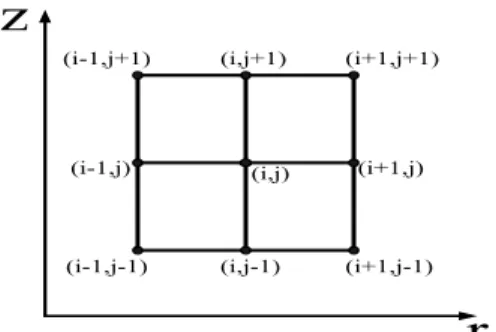
(2.7)-Figure 1: A nine-point compact stencil. (2.9) and (2.5), we obtain the following difference scheme

δ2 rUi,j − ∆r2 12 [δ 2 rFi,j − 1 ri δ1 rFi,j + 3 + n2 r2 i δ2 rUi,j − 3 + 5n2 r3 i δ1 rUi,j +8n2 r4 i Ui,j+ 1 ri δ1 rδz2Ui,j − δr2δ2zUi,j] + 1 ri δ1 rUi,j −∆r2 6ri [δ1 rFi,j − 1 ri δ2 rUi,j+ 1 + n2 r2 i δ1 rUi,j− 2n2 r3 i Ui,j − δr1δ2zUi,j] − n2 r2 i Ui,j +δ_z2Ui,j − ∆z2 12 [δ 2 zFi,j− δ2zδr2Ui,j− 1 ri δ2_zδ_r1Ui,j+ n2 r2 i δ2_zUi,j] = Fi,j, (2.16)

for 1 ≤ i ≤ L, 1 ≤ j ≤ M. Note that, the scheme involves centered difference approximations to first or second order partial derivatives in r and z so only a nine-point compact stencil is used, see the Figure 1 for illustration. One can also see that if the order terms of ∆r2 _{and ∆z}2 _{are ignored in the equation (2.16), then the}

scheme recovers to the usual second-order accurate scheme as in [2].

In order to close the linear system, the numerical boundary values U0,j, UL+1,j

and Ui,0, Ui,M +1 should be supplied. The numerical boundary value U0,j can be

given by U0,j = (−1)nU1,j due to the symmetry constraint of Fourier coefficients

(ˆun(−∆r/2, zj) = (−1)nuˆn(∆r/2, zj)) [3]. And the other numerical boundary can be

easily obtained by the given Dirichlet boundary values UL+1,j= ˆunS(zj), Ui,0 = ˆunB(ri)

2.3

Numerical results

In this subsection, we perform some numerical tests on the accuracy and efficiency of our scheme. Since the matrix of the resultant linear system in (2.16) is nonsym-metric, we use the BiConjugate Gradient Stabilized method (Bi-CGSTAB) [10] to solve the linear systems. The stopping criterion of the convergence is based on the relative residual which the tolerance ranges from 10−9 _{− 10}−13 _{depending on the}

different Fourier modes.

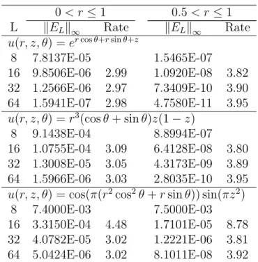
Table 1 shows the maximum relative errors for three different solutions of Poisson equation in cylindrical coordinates. In all our tests, we use L mesh points in the radial (r) and axial (z) directions, and 2L points in the azimuthal (θ) direction. The rate of convergence is computed by the formula log₂(EL/2

EL ), where EL is the maximum relative error with mesh resolution L.

From Table 1, we can see that the errors of the solutions show third-order con-vergence for all examples in the case of solid cylinder (0 < r ≤ 1). The loss of one order of accuracy seems to come from the discretization near the polar origin. This can be seen from the following truncation error analysis. In the Fourier mode equation (2.5), the Ur(= ∂ ˆun/∂r) term is divided by r. So the second-order

approx-imation of Urrr in (2.7) is divided by an O(∆r) term near the origin, which makes

the approximation of Urrr/r first-order accurate. This has the consequence that the

overall truncation error of the Ur/r term in the vicinity of the origin is O(∆r3) and

thus so is the Fourier mode equation (2.5). However, this loss of accuracy does not appear when solving the problem on a cylinder that excludes the polar singularity such as the case of 0 < a ≤ r ≤ 1. Let us explain why is the case next.

As in the solid cylinder case, we need to solve Eq.(2.5) with the Dirichlet bound-ary condition at r = 1 and an additional boundbound-ary condition imposed at r = a. Instead of setting a grid as in (2.12), we choose a regular grid in the radial direction as

ri = a + i∆r, i = 0, 1, ..., L, L + 1, (2.17)

with the mesh width ∆r = (1 − a)/(L + 1). Now the second-order approximation of Urrr in (2.7) is divided by an O(a + ∆r) term instead of an O(∆r) term, so the

truncation error of the Urrr/r term is still O(∆r2) which makes the discretization

error of Ur/r term is O(∆r4). Therefore, the overall truncation error of Eq.(2.5) is

O(∆r4_{). One can see in Table 1 that the fourth-order convergence indeed can be}

achieved for all test examples for the case of 0.5 ≤ r ≤ 1.

In order to speed up the convergence of Bi-CGSTAB iteration, we have applied different preconditioners which include Block Jacobi (BJ) [8], Incomplete LU fac-torization (ILU) [8], and the Fast Direct Solver (FDS) arising from the second-order discretization for the equation (2.5) which is developed in [2]. Here, we solve the difference equation (2.16) with the Fourier mode number n = 1. The tolerance for the relative residual is chosen as 10−9_.

0 < r ≤ 1 0.5 < r ≤ 1

L kELk∞ Rate kELk∞ Rate

u(r, z, θ) = er cos θ+r sin θ+z

8 7.8137E-05 1.5465E-07

16 9.8506E-06 2.99 1.0920E-08 3.82 32 1.2566E-06 2.97 7.3409E-10 3.90 64 1.5941E-07 2.98 4.7580E-11 3.95

u(r, z, θ) = r3_{(cos θ + sin θ)z(1 − z)}

8 9.1438E-04 8.8994E-07

16 1.0755E-04 3.09 6.4128E-08 3.80 32 1.3008E-05 3.05 4.3173E-09 3.89 64 1.5966E-06 3.03 2.8035E-10 3.95

u(r, z, θ) = cos(π(r2_cos2_{θ + r sin θ)) sin(πz}2₎

8 7.4000E-03 7.5000E-03

16 3.3150E-04 4.48 1.7101E-05 8.78 32 4.0782E-05 3.02 1.2221E-06 3.81 64 5.0424E-06 3.02 8.1011E-08 3.92

Table 1: The maximum relative errors for different solutions to Poisson equation in cylindrical coordinates.

Table 2 shows the number of iterations needed to be convergent for different preconditioners applied to Bi-CGSTAB iteration. The column of ”Bi-CGSTAB” is the one without any preconditioner which, as expected, has the largest number of iterations. The preconditioners BJ and ILU both need double iterations when the grid points are doubled. One can see that, the FDS preconditioner turns out to be the most efficient one since it has the least number of iterations, and the iterations are kept to be a constant when we double the grid points.

L Bi-CGSTAB BJ ILU FDS

8 25 16 6 7

16 52 34 9 7

32 97 65 19 7

64 182 134 38 7

Table 2: The performance comparison of different preconditioners for the cylindrical case.

3

Poisson equation in 3D spherical coordinates

In this section, we perform the similar derivation as the cylindrical case and develop a spectral/finite difference scheme for Poisson equation in 3D spherical domain. The Poisson equation with Dirichlet boundary in a spherical shell Ω = {R0 ≤ ρ ≤ 1, 0 ≤

φ ≤ π, 0 ≤ θ ≤ 2π} can be written in spherical coordinates as ∂2_u ∂ρ2 + 2 ρ ∂u ∂ρ + 1 ρ2 ∂2_u ∂φ2 + cot φ ρ2 ∂u ∂φ+ 1 ρ2_sin2_φ ∂2_u ∂θ2 = f (ρ, φ, θ), (3.18) u(R0, φ, θ) = uI(φ, θ), u(1, φ, θ) = uS(φ, θ). (3.19)

Here, the boundary condition should be imposed on the inner (ρ = R0 > 0) and

outer (ρ = 1) surfaces of the sphere.

As the cylindrical case, the main difficulty for solving Eq.(3.18) is to treat the coordinate singularities along the polar axis where north (φ = 0) and south (φ = π) poles are located. Most of numerical approaches including finite difference and spectral methods involve imposing additional pole conditions to capture the behavior of the solution in the vicinity of the poles. In [1, 2], we have developed a series of FFT-based second-order fast Poisson solver without pole conditions for 2D and 3D spherical domains. In the following, we will develop a formally fourth-order compact scheme for Eqs. (3.18)-(3.19). To the best of our knowledge, we have not seen any related work in the literature.

3.1

Fourier mode equations

As in the cylindrical coordinate case, we approximate u by the truncated Fourier series as u(ρ, φ, θ) = N/2−1_X n=−N/2 ˆ un(ρ, φ) einθ, (3.20)

where ˆun(ρ, φ) is the complex Fourier coefficient given by

ˆ un(ρ, φ) = 1 N N −1_X k=0 u(ρ, φ, θk) e−inθk, (3.21)

and θk = 2kπ/N and N is the number of grid points along a latitude circle. Once

again, the above transformation between the physical space and Fourier space can be efficiently performed by the Fast Fourier Transform (FFT) with O(N log₂N)

arithmetic operations. The expansion for the function f can be written in the similar fashion.

Substituting those expansions into Eq.(3.18), and equating the Fourier coeffi-cients, ˆun(ρ, φ) then satisfies the PDE

∂2_uˆ n ∂ρ2 + 2 ρ ∂ ˆun ∂ρ + 1 ρ2 ∂2_uˆ n ∂φ2 + cot φ ρ2 ∂ ˆun ∂φ − n2 ρ2_sin2_φuˆn= ˆfn(ρ, φ), (3.22) ˆ un(R0, φ) = ˆunI(φ), uˆn(1, φ) = ˆunS(φ). (3.23) Here, ˆun

I(φ) and ˆunS(φ) are the nth Fourier coefficient of uI(φ, θ) and uS(φ, θ),

re-spectively. Next, we need to derive a formally fourth-order compact scheme for the Fourier mode equations (3.22).

3.2

Formally fourth-order compact difference discretization

As in [2], we choose a grid in (ρ, φ) plane by

ρi = R0+ i ∆r, φj = (j − 1/2) ∆φ, (3.24)

for 0 ≤ i ≤ L + 1, 0 ≤ j ≤ M + 1 with ∆ρ = (1 − R0)/(L + 1) and ∆φ = π/M. By

the choice of those mesh points, we avoid placing points directly at north (φ = 0) and south (φ = π) poles. Again, let the discrete values be denoted by U(ρi, φj) ≈

ˆ

un(ρi, φj), and F (ρi, φj) ≈ ˆfn(ρi, φj).

Our goal is to derive a fourth-order finite difference approximation to Eq.(3.22). Obviously, the first and second derivatives, Uρ, Uρρ, Uφ and Uφφ must be

approx-imated to fourth-order accurately. In order to have fourth-order approximations for Uρ, Uρρ, Uφ and Uφφ, we need to approximate the higher order derivatives Uρρρ,

Uρρρρ, Uφφφ and Uφφφφ to be second-order accurate. We then reduce those higher

order partial derivatives to lower order by differentiating the equation (3.22) and use the regular centered difference to approximate those lower order partial deriva-tives. The derivation is very similar to the cylindrical case, so we omit the detail here. After a tedious calculation, we obtain a finite difference scheme as follows.

For 1 ≤ i ≤ L, 1 ≤ j ≤ M, we have δ_ρ2Ui,j− ∆ρ 2 12 [δ 2 ρFi,j − 2 ρi δ_ρ1Fi,j + (8 + n 2_csc2_φ j ρ2 i )δ_ρ2Ui,j+ 10n 2_csc2_φ j ρ4 i Ui,j +(−8 − 6n 2_csc2_φ j ρ3 i )δ1 ρUi,j − 10 ρ4 i δ2 φUi,j− 10 cot φj ρ4 i δ1 φUi,j+ 6 cot φj ρ3 i δ1 ρδφ1Ui,j + 6 ρ3 i δ1 ρδφ2Ui,j − cot φj ρ2 i δ2 ρδφ1Ui,j − 1 ρ2 i δ2 ρδ2φUi,j] + 2 ρi {δ1 ρUi,j− ∆r2 6 [δ 1 ρFi,j −2 ρi δ2 ρUi,j+ ( 2 + n2_csc2_φ j ρ2 i )δ1 ρUi,j+ 2 cot φj ρ3 i δ1 φUi,j+ 2 ρ3 i δ2 φUi,j − cot φj ρ2 i δ1 ρδφ1Ui,j − 1 ρ2 i δ_ρ1δ_φ2Ui,j− 2n2_csc2_φ j ρ3 i Ui,j]} + 1 ρ2 i {δ_φ2Ui,j − ∆φ2 12 [ρ 2

iδφ2Fi,j− ρ2i cot φjδφ1Fi,j

+((3 + n2) csc2φj− 1)δφ2Ui,j+ (−3 − 5n2) csc2φjcot φjδφ1Ui,j

+2n2_csc2_φ

j(4 csc2φj− 3)Ui,j+ 2ρicot φjδ1φδρ1Ui,j+ ρ2i cot φjδφ1δρ2Ui,j

−2ρiδφ2δρ1Ui,j− ρ2iδφ2δρ2Ui,j]} + cot φj ρ2 i {δ1 φUi,j− ∆φ2 6 [−ρ 2 iδ1φδ2ρUi,j − 2ρiδφ1δρ1Ui,j +(1 + n2_{) csc}2_φ

jδφ1Ui,j − cot φjδ2φUi,j− 2n2csc2φjcot φjUi,j+ ρ2iδ1φFi,j]}

−n2csc2φj ρ2

i

Ui,j = Fi,j. (3.25)

Note that, the scheme involves centered difference approximations to first or second order partial derivatives in ρ and φ so only a nine-point compact stencil is used. One can also see that if the order terms of ∆ρ2 _{and ∆φ}2 _{are ignored in the equation}

(3.25), then the scheme recovers to the usual second-order accurate scheme as in [2]. When j = 1 for Eq.(3.25), the numerical boundary value Ui,0 can be given by

Ui,0 = (−1)nUi,1. This is because the Fourier coefficient satisfies the symmetry

constraint ˆun(ρi, −∆φ/2) = (−1)nuˆn(ρi, ∆φ/2) [2]. Similarly, another numerical

boundary value Ui,M +1 can also be obtained by Ui,M +1 = (−1)nUi,M for the same

reason. So the numerical boundary values in the φ direction are provided and no pole condition is needed in our finite difference setting. The other numerical boundary

U0,j, UL+1,j are given by the boundary values ˆunI(φj), ˆunS(φj).

3.3

Numerical results

In this subsection, we perform similar numerical tests on the accuracy and efficiency of our scheme for the spherical coordinates case. In all our tests, we use L mesh points in the radial (ρ) and colatitude (φ) directions, and 2L points in the longitude (θ) direction. The inner radius is chosen as R0 = 0.5. The difference equation (3.25)

stopping ranges from 10−9_{− 10}−13 _{depending on the different Fourier modes. Once}

we obtain the Fourier coefficients, the numerical solution can be computed by the inverse FFT as in (3.20). Table 3 shows the maximum errors of the method for three different solutions of Poisson equation in a spherical shell. One can see that the errors of the solutions show third-order convergence for all test examples. The reason of losing one order of accuracy is exactly the same as the cylindrical case so we omit the discussion here.

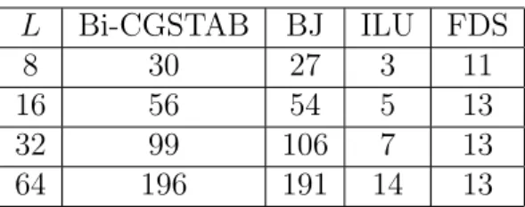
Table 4 shows the number of iterations needed for solving the difference equation (3.25) of n = 1 by the Bi-CGSTAB method with different preconditioners. The tolerance of stopping for the relative residual is chosen as 10−9_{. Generally speaking,}

the performance of those preconditioners are almost the same as the cylindrical case. It is interesting to see that the ILU preconditioner seems to have the less number of iterations than the FDS when the number of grid points is small. However, the ILU does increase the iterations as the grid points increasing while the FDS preconditioner still keeps the number of iterations.

L kELk∞ Rate

u(ρ, φ, θ) = eρ sin φ cos θ+ρ sin φ sin θ+ρ cos φ

8 3.7000E-03

16 5.4095E-04 2.77

32 7.4825E-05 2.85

64 1.0067E-05 2.89

u(ρ, φ, θ) = ρ3_{(cos θ + sin θ) sin φ(1 − ρ cos φ)}

8 5.2000E-03

16 9.5143E-04 2.45

32 1.5249E-04 2.64

64 2.2549E-05 2.76

u(ρ, φ, θ) = cos(π(ρ2_cos2_{θ sin}2_{φ + ρ sin θ sin φ)) sin(πρ}2_cos2_φ)

8 5.3700E-02

16 7.1000E-03 2.92

32 8.3568E-04 3.09

64 9.7240E-05 3.10

Table 3: The maximum relative errors for different solutions to Poisson equation in spherical coordinates.

4

Conclusion and acknowledgement

In this paper, we present a formally fourth-order compact difference scheme for 3D Poisson equation in cylindrical and spherical coordinates. The solver relies on the

L Bi-CGSTAB BJ ILU FDS

8 30 27 3 11

16 56 54 5 13

32 99 106 7 13

64 196 191 14 13

Table 4: The performance comparison of different preconditioners for the spherical case.

truncated Fourier series expansion, where the partial differential equations of Fourier coefficients are solved by a formal fourth-order compact difference discretizations without pole conditions. The resultant linear system is then solved by the Bi-CGSTAB method with different preconditioners. The numerical results confirm the formal accuracy of our scheme. Meanwhile, the preconditioner arising from the second-order fast direct solver shows the scalability of Bi-CGSTAB with the problem size.

The authors are supported in part by the National Science council of Taiwan under research grant NSC-93-2115-M-009-008.

References

[1] M.-C. Lai and W.-C. Wang, Fast direct solvers for Poisson equation on 2D polar and spherical gepmetries. Numer. Meth. Partial Diff. Eq., 18, 56-68, (2002). [2] M.-C. Lai, W.-W. Lin and W. Wang, A fast spectral/difference method without

pole conditions for Poisson-type equations in cylindrical and spherical geome-tries. IMA J. Numer. Anal., 22, 537-548, (2002).

[3] M.-C. Lai, A simple compact fourth-order Poisson solver on polar geometry. J.

Comput. Phys., 182, 337-345, (2002).

[4] R. C. Mittal and S. Gahlaut, High-order finite-difference schemes to solve Pois-son’s equation in polar coordinates, IMA J. Numer. Anal., 11, 261, (1991). [5] M. K. Jain, R. K. Jain and M. Krishna, A fourth-order difference scheme for

quasilinear Poisson equation in polar co-ordinates, Communications in

Numer-ical Methods in Engineering, vol. 10, 791-797 (1994).

[6] S. R. K. Iyengar and R. Manohar, High order difference methods for heat equation in polar cylindrical coordinates, J. Comput. Phys., 77, 425 (1988).

[7] S. R. K. Iyengar and A. Goyal, A note on multigrid for the three-dimensional Poisson equation in cylindrical coordinates, J. Comput. Appl. Math., 33, 163-169, (1990).

[8] B. Richard et al. Templates for the solution of linear systems:Building blocks

for iterative methods, SIAM (1994).

[9] J. C. Strikwerda, Finite Difference schemes and Partial Differential Equations, Page 286-287, Wadsworth & Brooks/Cole, (1989).

[10] H. A. Van der Vorst, Bi-CGSTAB : A fast and smoothly converging variant of Bi-CG for the solution of nonsymmetric linear systems. SIAM J. Sci. Statist.